
Essence of Structure Preserving (ESP) Network Reductions for Engineering and Economic ... · ·...
61
Essence of Structure Preserving (ESP) Network Reductions for Engineering and Economic Analysis 1 Dan Tylavsky, Yingying Qi, Yujia Zhu, Di Shi Arizona State University with William Schulze, Ray Zimmerman, Dick Shuler, Jubo Yan Cornell University Dan Shawhan Rensselaer Polytechnic University CERTS R&M Cornell Aug 6-7, 2013
Transcript of Essence of Structure Preserving (ESP) Network Reductions for Engineering and Economic ... · ·...
Essence of Structure Preserving (ESP) Network Reductions for Engineering and Economic
Analysis
1
Dan Tylavsky, Yingying Qi, Yujia Zhu, Di Shi
Arizona State University
with William Schulze, Ray Zimmerman, Dick Shuler, Jubo Yan
Cornell University
Dan Shawhan Rensselaer Polytechnic University
CERTS R&M Cornell Aug 6-7, 2013
Overview • 1: Supporting Cornell SuperOPF studies of the US power
system. • 2: Porting Modified-Ward reduction method to the public
domain. • 3: Overarching Motivation-develop network equivalents that
preserved structure for different applications. • Inter-zonal-flow preserving network equivalents.
– Bus Aggregation methods for accurate inter-area power flow calculations.
– (Review) Bus-Aggregation using PTDF’s – Clustering – Equivalent branch reactances – Accuracy
– Computation time minimization—effect on accuracy – Comparison of PTDF calculation assumptions – Results of Reduction (Accuracy)
• Conclusions
Supporting SuperOPF Studies
• Supporting Cornell SuperOPF studies. – Developing network reductions using Modified
Ward method. – Using WECC, EI, ERCOT. – Different size reduced equivalents. – Different base-case reduced equivalents. – Validations for accuracy.
• Branch flows—base case, change-cases. • OPF—metrics on LMP, objective function.
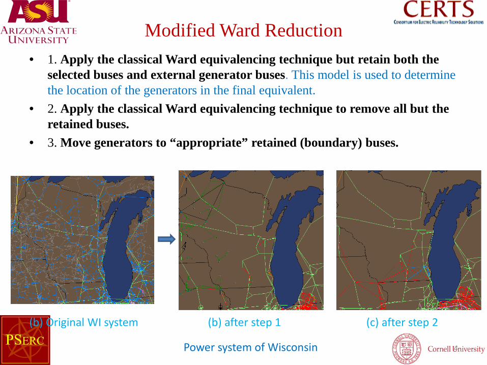
• 1. Apply the classical Ward equivalencing technique but retain both the selected buses and external generator buses. This model is used to determine the location of the generators in the final equivalent.
• 2. Apply the classical Ward equivalencing technique to remove all but the retained buses.
• 3. Move generators to “appropriate” retained (boundary) buses.
4 Power system of Wisconsin
(b) after step 1 (c) after step 2 (b) Original WI system
Modified Ward Reduction
The Shortest Path Problem
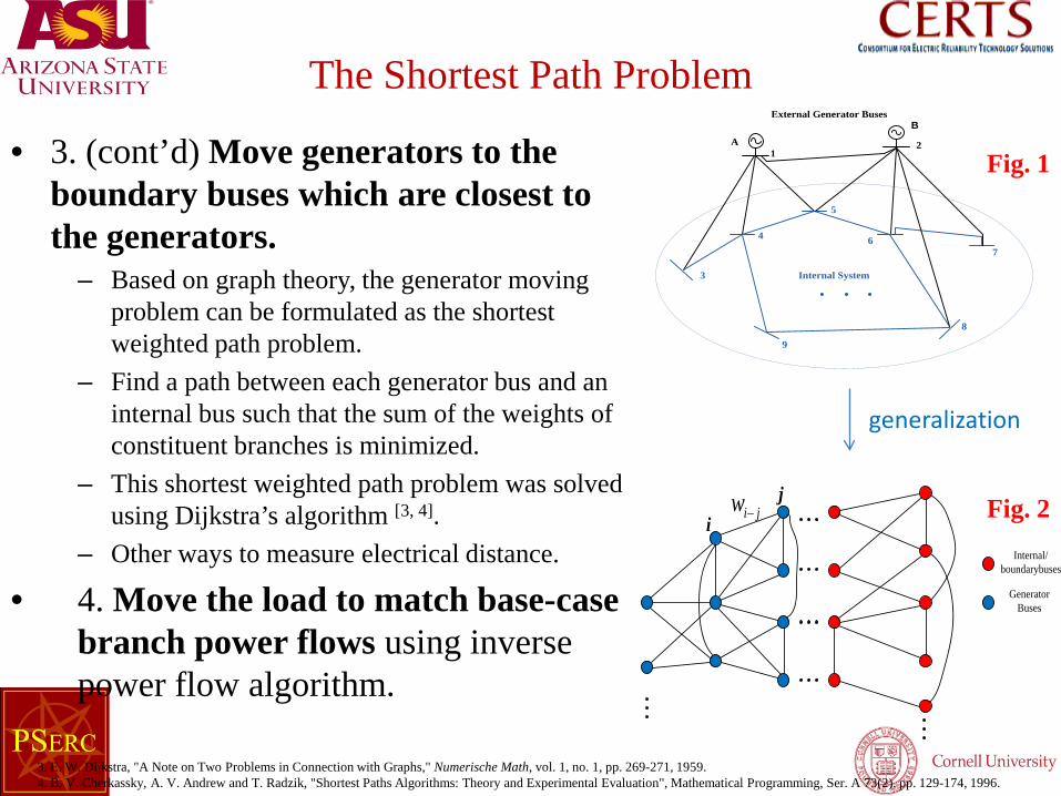
• 3. (cont’d) Move generators to the boundary buses which are closest to the generators.
– Based on graph theory, the generator moving problem can be formulated as the shortest weighted path problem.
– Find a path between each generator bus and an internal bus such that the sum of the weights of constituent branches is minimized.
– This shortest weighted path problem was solved using Dijkstra’s algorithm [3, 4].
– Other ways to measure electrical distance.
• 4. Move the load to match base-case branch power flows using inverse power flow algorithm.
12
3
4
5
67
8
9
Internal System
External Generator Buses
A
B
ij
jiw −
Internal/boundarybuses
Generator Buses
generalization
Fig. 1
Fig. 2
3. E. W. Dijkstra, "A Note on Two Problems in Connection with Graphs," Numerische Math, vol. 1, no. 1, pp. 269-271, 1959. 4. B. V. Cherkassky, A. V. Andrew and T. Radzik, "Shortest Paths Algorithms: Theory and Experimental Evaluation", Mathematical Programming, Ser. A 73(2), pp. 129-174, 1996.
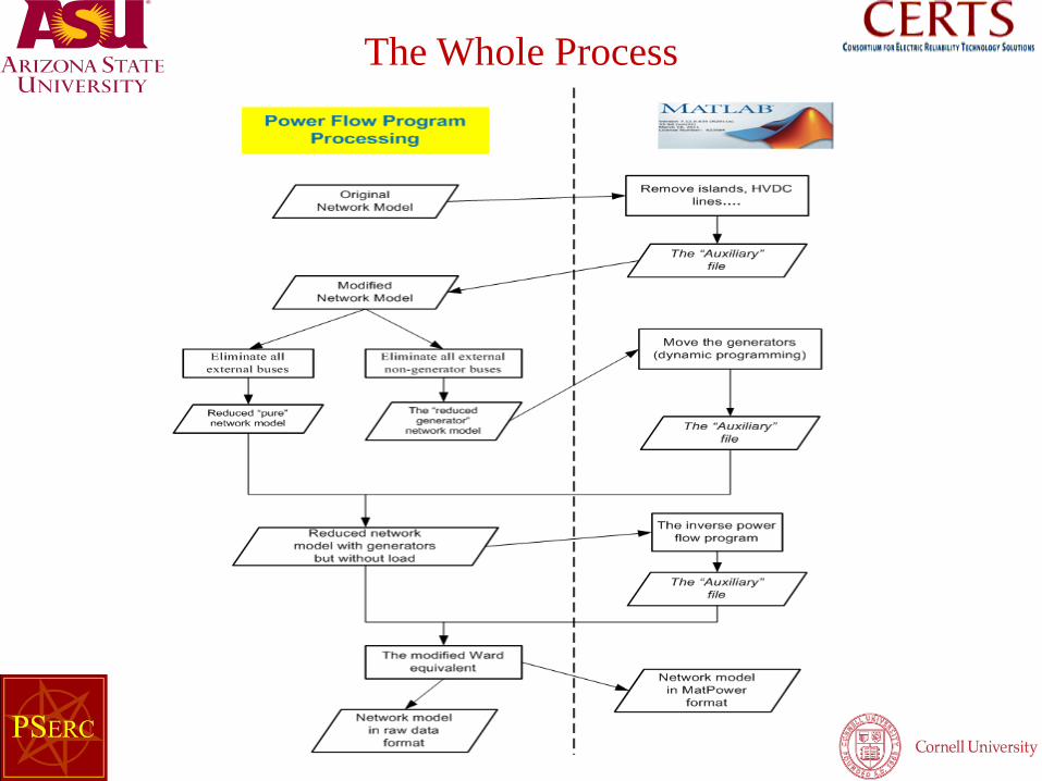
The Whole Process
The Modified Ward Equivalent
• Thrust #1—Bring Modified-Ward equivalencing procedure to public domain—Bob Thomas. (Continuation of FY12)
• Objectives: – User intervention in the process should be
minimized. – All completed using one power-flow application—
MatPower. – Testing to prevent crashes.
7

Moving Modified Ward Equivalent to Public Domain • Major tasks for removing the seams between
the following discrete steps – Data Conversion (Completed) – Island Identification & HVDC treatment (In progress) – Data Quality Control (In progress) – Network Reduction – Generator Assignment – Load Assignment – Output—PSSE? PSSE and PowerWorld?? – Testing – User’s Manual
8
Porting Modified Ward Equivalent to Public Domain • Data conversion challenges
– Design application to work with PSSE and PowerWorld input format.
– Reading in the PSS/E .raw format data • Different data formats, e.g., two winding v. three-winding xfmrs. • Adapting model differences, e.g., control of switched shunts. • Adding fictitious buses, e.g., star point of three-winding
transformers. • Validation with large datasets is time consuming.
9
Bus Aggregation A Different Approach
• FY 2012—Bus aggregation techniques: Goal is to preserve inter-zonal power flows to accurately model system behavior under bilateral transactions.
• Difference from modified Ward: – dc rather than ac model reduction. – Aggregate buses rather than “eliminate” buses. – Match base-case inter-zonal flows accurately,
(rather than retained transmission line flows as in modified Ward.)
10
Bus Aggregation A Different Approach
• FY 2013—Continue bus aggregation to its logical conclusion.
• Thrust #2: Improving computational efficiency • Thrust #3: Improve accuracy
11
Bus Aggregation
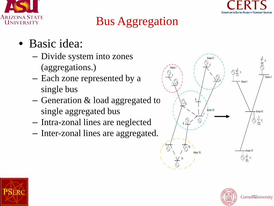
• Basic idea: – Divide system into zones
(aggregations.) – Each zone represented by a
single bus – Generation & load aggregated to
single aggregated bus – Intra-zonal lines are neglected – Inter-zonal lines are aggregated.
12
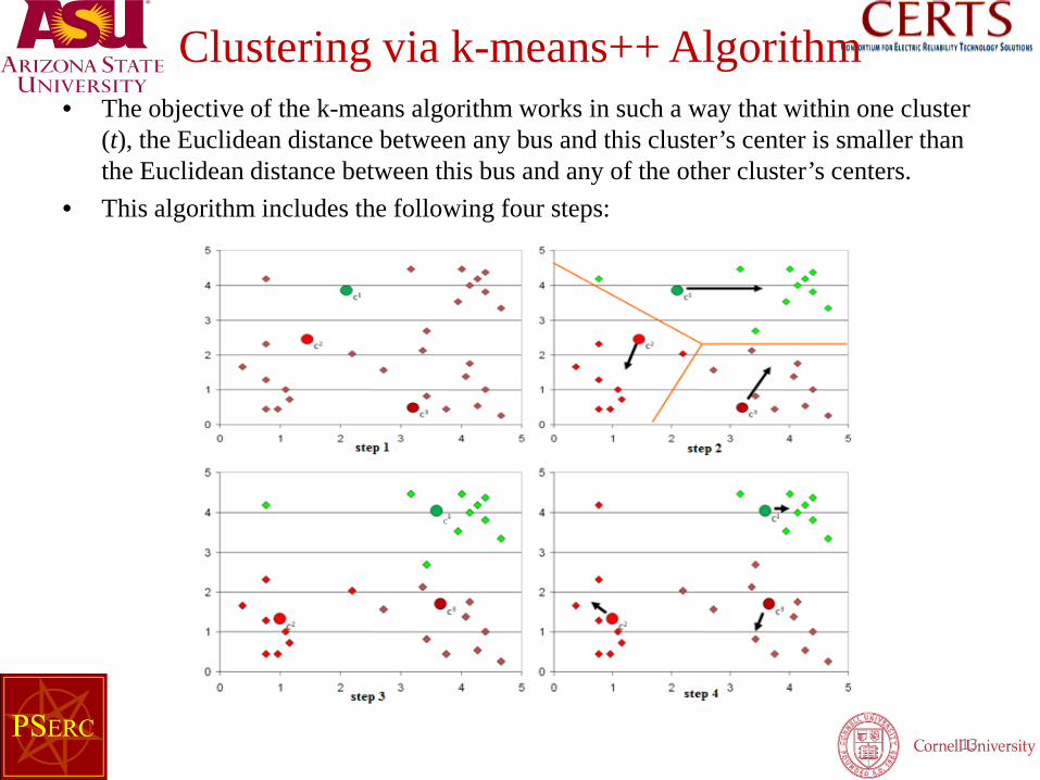
Clustering via k-means++ Algorithm • The objective of the k-means algorithm works in such a way that within one cluster
(t), the Euclidean distance between any bus and this cluster’s center is smaller than the Euclidean distance between this bus and any of the other cluster’s centers.
• This algorithm includes the following four steps:
13
Power Transfer Distribution Factor (PTDF)
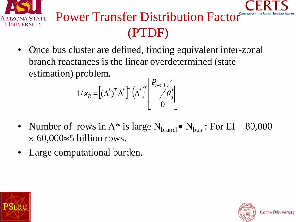
• Once bus cluster are defined, finding equivalent inter-zonal branch reactances is the linear overdetermined (state estimation) problem.
14
• Number of rows in Λ* is large Nbranch• Nbus : For EI—80,000 × 60,000≈5 billion rows.
• Large computational burden.
[ ] ( )
ΛΛΛ=
>−−
0)(/1 **1**
ij
jiTTR
Px θ
The Over-Determined Problem
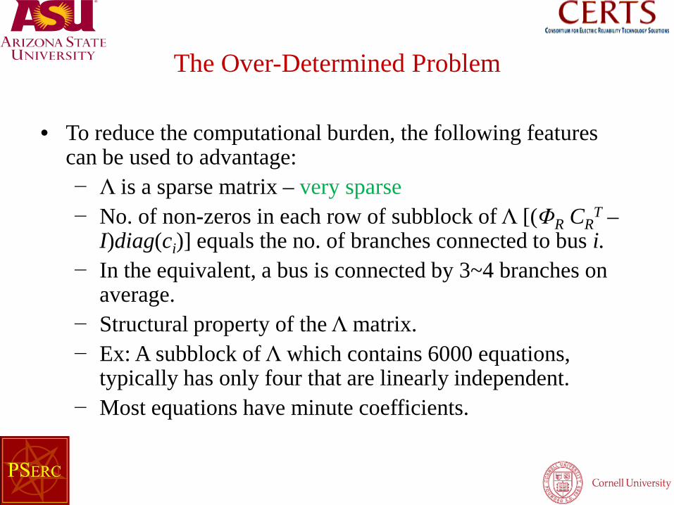
• To reduce the computational burden, the following features can be used to advantage: − Λ is a sparse matrix – very sparse − No. of non-zeros in each row of subblock of Λ [(ΦR CR
T –I)diag(ci)] equals the no. of branches connected to bus i.
− In the equivalent, a bus is connected by 3~4 branches on average.
− Structural property of the Λ matrix. − Ex: A subblock of Λ which contains 6000 equations,
typically has only four that are linearly independent. − Most equations have minute coefficients.

Equation Selection
• To reduce dimension of Λ, eliminate equations whose coefficients are below a threshold.
• Compare branch reactance and flow errors as a function of threshold values for reduced dc model.
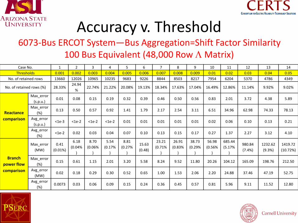
Accuracy v. Threshold 6073-Bus ERCOT System—Bus Aggregation=Shift Factor Similarity
100 Bus Equivalent (48,000 Row Λ Matrix) Case No. 1 2 3 4 5 6 7 8 9 10 11 12 13 14
Thresholds 0.001 0.002 0.003 0.004 0.005 0.006 0.007 0.008 0.009 0.01 0.02 0.03 0.04 0.05 No. of retained rows 13660 12026 10965 10235 9683 9226 8844 8503 8217 7954 6204 5370 4786 4349
No. of retained rows (%) 28.33% 24.94
% 22.74% 21.22% 20.08% 19.13% 18.34% 17.63% 17.04% 16.49% 12.86% 11.14% 9.92% 9.02%
Reactance comparison
Max_error (s.p.u.)
0.01 0.08 0.15 0.19 0.32 0.39 0.46 0.50 0.56 0.83 2.01 3.72 4.38 5.89
Max_error (%)
0.13 0.50 0.57 0.92 1.41 1.79 2.17 2.54 3.11 6.51 34.96 62.98 74.33 78.13
Avg_error (s.p.u.)
<1e-3 <1e-2 <1e-2 <1e-2 0.01 0.01 0.01 0.01 0.01 0.02 0.06 0.10 0.13 0.21
Avg_error (%)
<1e-2 0.02 0.03 0.04 0.07 0.10 0.13 0.15 0.17 0.27 1.37 2.27 3.12 4.10
Branch power flow comparison
Max_error (MW)
0.41 (0.01%)
6.18 (0.04%
)
8.70 (0.06%
)
5.54 (0.17%
)
8.81 (0.27%
)
15.63 (0.48)
23.21 (0.71%
)
26.91 (0.83%
)
38.73 (0.29%
)
56.98 (0.56%
)
685.44 (5.17%
)
980.84 (7.4%)
1232.62 (9.3%)
1419.72 (10.72%)
Max_error (%)
0.15 0.61 1.15 2.01 3.20 5.58 8.24 9.52 11.80 20.26 104.12 165.09 198.76 212.50
Avg_error (MW)
0.02 0.18 0.29 0.30 0.52 0.65 1.00 1.53 2.06 2.20 24.88 37.46 47.19 52.75
Avg_error (%)
0.0073 0.03 0.06 0.09 0.15 0.24 0.36 0.45 0.57 0.81 5.96 9.11 11.52 12.80
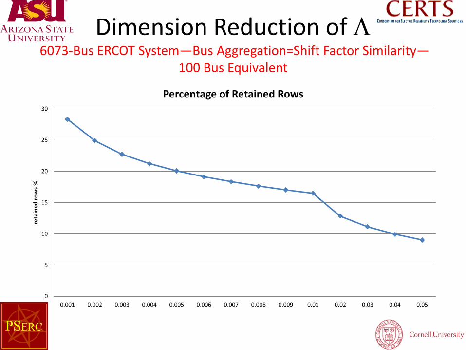
Dimension Reduction of Λ 6073-Bus ERCOT System—Bus Aggregation=Shift Factor Similarity—
100 Bus Equivalent
0
5
10
15
20
25
30
0.001 0.002 0.003 0.004 0.005 0.006 0.007 0.008 0.009 0.01 0.02 0.03 0.04 0.05
reta
ined
row
s %
Percentage of Retained Rows
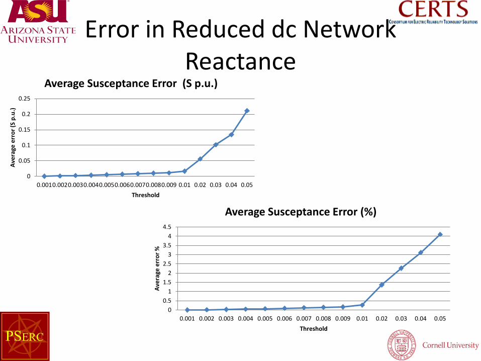
Error in Reduced dc Network Reactance
0
0.05
0.1
0.15
0.2
0.25
0.001 0.002 0.003 0.004 0.005 0.006 0.007 0.008 0.009 0.01 0.02 0.03 0.04 0.05
Aver
age
erro
r (S
p.u.
)
Threshold
Average Susceptance Error (S p.u.)
0 0.5
1 1.5
2 2.5
3 3.5
4 4.5
0.001 0.002 0.003 0.004 0.005 0.006 0.007 0.008 0.009 0.01 0.02 0.03 0.04 0.05
Aver
age
erro
r %
Threshold
Average Susceptance Error (%)
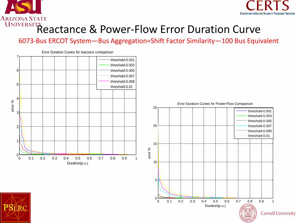
Reactance & Power-Flow Error Duration Curve 6073-Bus ERCOT System—Bus Aggregation=Shift Factor Similarity—100 Bus Equivalent
0 0.1 0.2 0.3 0.4 0.5 0.6 0.7 0.8 0.9 10
1
2
3
4
5
6
7
Duration(p.u.)
erro
r %
Error Duration Curves for reactace comparison
threshold-0.001threshold-0.003threshold-0.005threshold-0.007threshold-0.009threshold-0.01
0 0.1 0.2 0.3 0.4 0.5 0.6 0.7 0.8 0.9 10
5
10
15
20
25
Duration(p.u.)
erro
r %
Error Duration Curves for Power-Flow Comparison
threshold-0.001threshold-0.003threshold-0.005threshold-0.007threshold-0.009threshold-0.01
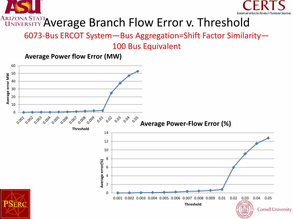
Average Branch Flow Error v. Threshold 6073-Bus ERCOT System—Bus Aggregation=Shift Factor Similarity—
100 Bus Equivalent
0
10
20
30
40
50
60
Ave
rage
err
or M
W
Threshold
Average Power flow Error (MW)
0
2
4
6
8
10
12
14
0.001 0.002 0.003 0.004 0.005 0.006 0.007 0.008 0.009 0.01 0.02 0.03 0.04 0.05
Aver
age
erro
r(%
)
Threshold
Average Power-Flow Error (%)
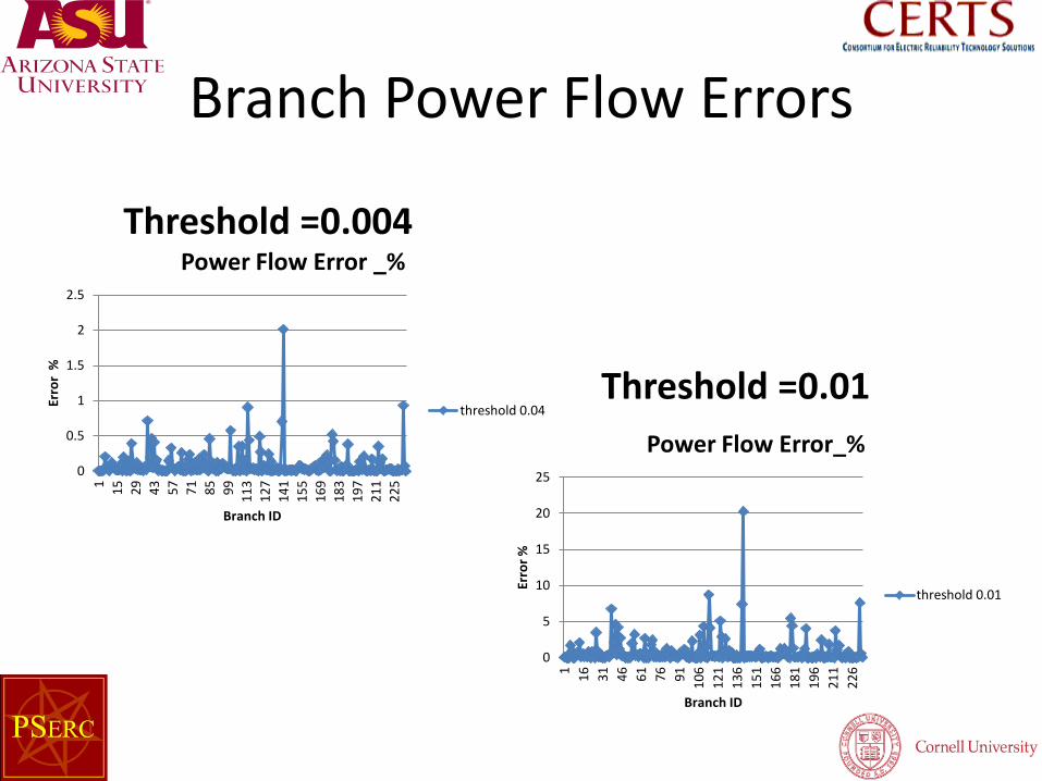
Branch Power Flow Errors
0
0.5
1
1.5
2
2.5
1 15
29
43
57
71
85
99
113
127
141
155
169
183
197
211
225
Erro
r %
Branch ID
Power Flow Error _%
threshold 0.04
0
5
10
15
20
25
1 16
31
46
61
76
91
106
121
136
151
166
181
196
211
226
Erro
r %
Branch ID
Power Flow Error_%
threshold 0.01
Threshold =0.004
Threshold =0.01
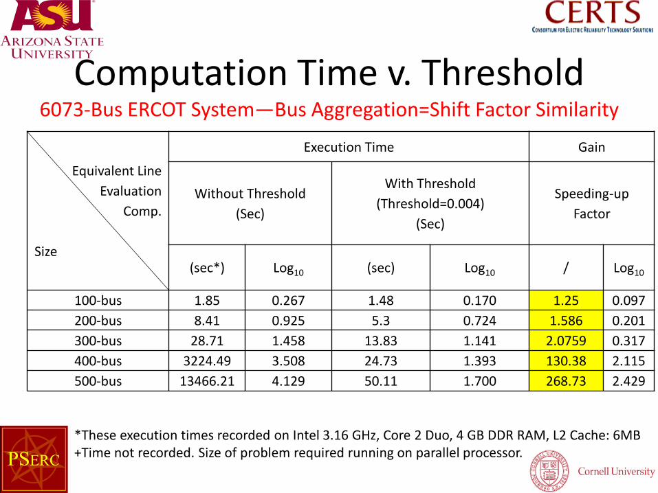
Equivalent Line Evaluation
Comp.
Size
Execution Time Gain
Without Threshold (Sec)
With Threshold (Threshold=0.004)
(Sec)
Speeding-up Factor
(sec*) Log10 (sec) Log10 / Log10
100-bus 1.85 0.267 1.48 0.170 1.25 0.097 200-bus 8.41 0.925 5.3 0.724 1.586 0.201 300-bus 28.71 1.458 13.83 1.141 2.0759 0.317 400-bus 3224.49 3.508 24.73 1.393 130.38 2.115 500-bus 13466.21 4.129 50.11 1.700 268.73 2.429
Computation Time v. Threshold 6073-Bus ERCOT System—Bus Aggregation=Shift Factor Similarity
*These execution times recorded on Intel 3.16 GHz, Core 2 Duo, 4 GB DDR RAM, L2 Cache: 6MB +Time not recorded. Size of problem required running on parallel processor.
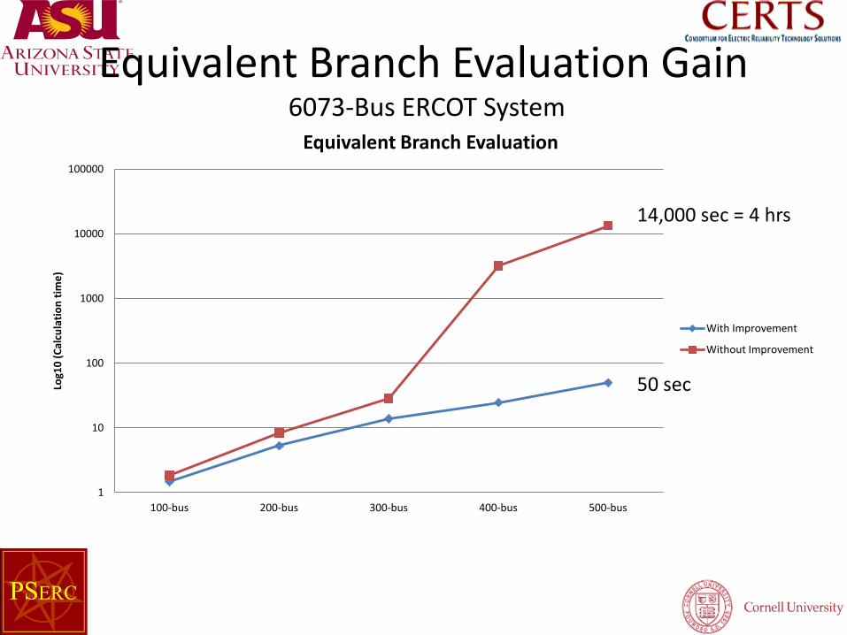
Equivalent Branch Evaluation Gain 6073-Bus ERCOT System
1
10
100
1000
10000
100000
100-bus 200-bus 300-bus 400-bus 500-bus
Log1
0 (C
alcu
latio
n tim
e)
Equivalent Branch Evaluation
With Improvement
Without Improvement
14,000 sec = 4 hrs
50 sec
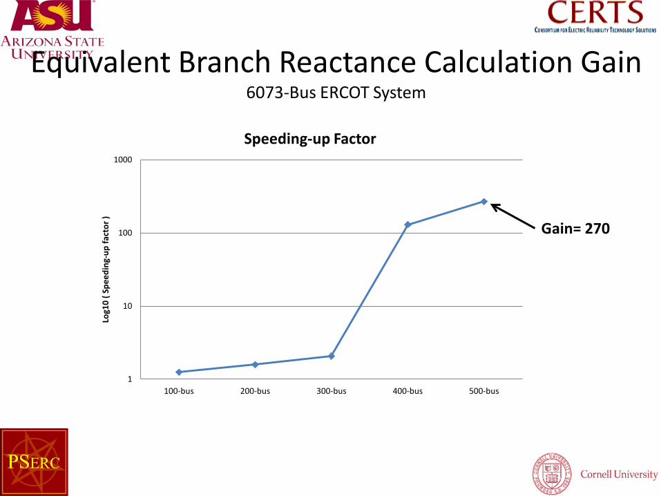
1
10
100
1000
100-bus 200-bus 300-bus 400-bus 500-bus
Log1
0 ( S
peed
ing-
up fa
ctor
)
Speeding-up Factor
Equivalent Branch Reactance Calculation Gain 6073-Bus ERCOT System
Gain= 270
Conclusions
• Using threshold values to eliminate a fraction of the redundant equations in the over-determined dc-network parameter estimation problem: – Has negligible effect on line flow accuracy. – Yields significant speed advantages. – Gives gains that grow exponentially with
size of reduced equivalent.
26
Thrust 3:Improving Bus-Aggregation Based Network Reduction Accuracy
• Thrust 3: Inter-zonal-flow preserving network equivalents.
• Central Concept for Improving Bus Aggregation Techniques for Network Reduction: – Don’t use classical dc-model PTDF’s. – Calculate accurate ac PTDF’s for unreduced model – Calculate “equivalent” dc PTDF’s for unreduced
model. – Use equivalent dc PTDF’s in the reduction.
27
Improving Bus Aggregation PTDF’s
• PTDF’s Nomenclature – Classical dc-model PTDF’s: – ac PTDF’s: Account for V, R, sin(θ).
• Are inconsistent. – dc PTDF’s: PTDF’s created from ac PTDF’s by
accounting for effect of power loss due to resistance. ⇒ Made consistent (approximately.)
28
1−= busbranchBBΦ
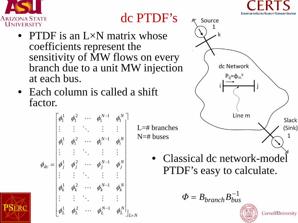
dc PTDF’s • PTDF is an L×N matrix whose
coefficients represent the sensitivity of MW flows on every branch due to a unit MW injection at each bus.
• Each column is called a shift factor.
29
L=# branches N=# buses
• Classical dc network-model PTDF’s easy to calculate.
1−= busbranch BBΦ
NLNL
NLLL
Nk
Nkkk
Nj
Njjj
Ni
Niii
NN
dc
×
−
−
−
−
−
=
φφφφ
φφφφ
φφφφ
φφφφ
φφφφ
φ
121
121
121
121
11
12
111
ac PTDF’s
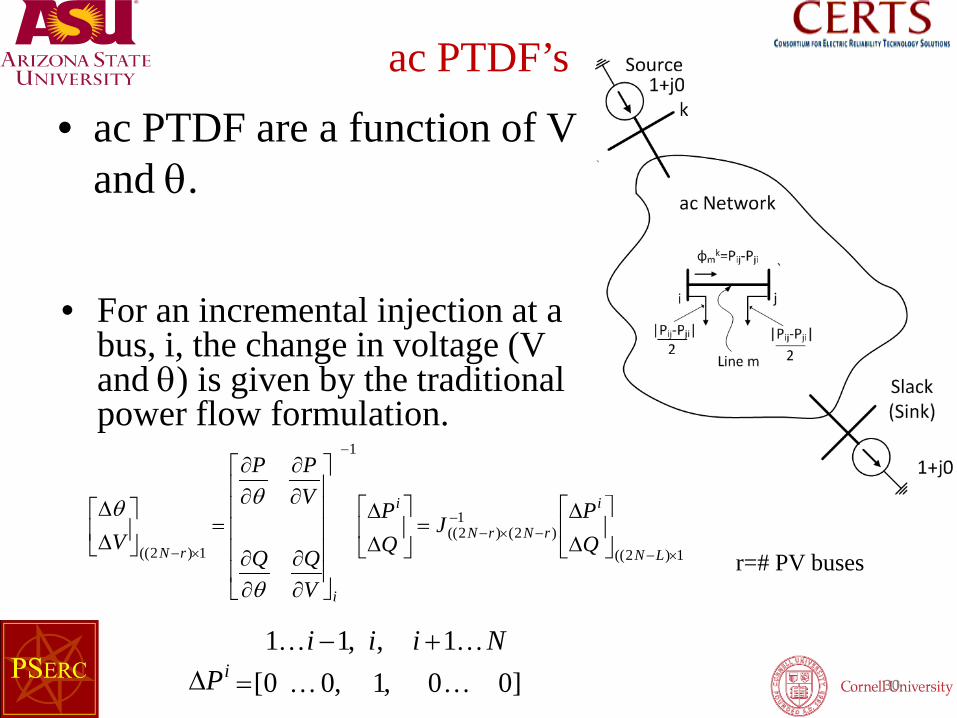
• ac PTDF are a function of V and θ.
30
• For an incremental injection at a bus, i, the change in voltage (V and θ) is given by the traditional power flow formulation.
]00,1,00[1,,11
NiiiPi
+−=∆
1)2((
1)2()2((
1
1)2(( ×−
−−×−
−
×−
∆∆
=
∆∆
∂∂
∂∂
∂∂
∂∂
=
∆∆
LN
i
rNrN
i
i
rN QPJ
QP
VQQ
VPP
V
θ
θθ
r=# PV buses
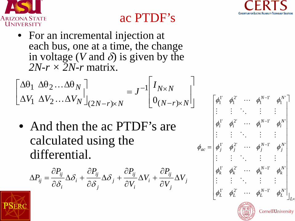
ac PTDF’s • For an incremental injection at
each bus, one at a time, the change in voltage (V and δ) is given by the 2N-r × 2N-r matrix.
31
• And then the ac PTDF’s are calculated using the differential.
=
∆∆∆
θ∆θ∆θ∆
×−
×−
×− NrN
NN
NrNN
N IJ
VVV )(
1
)2(21
21
0
jj
iji
i
ijj
j
iji
i
ijij V
VP
VVPPP
P ∆∂
∂+∆
∂
∂+∆
∂
∂+∆
∂
∂=∆ δ
δδ
δ
L
NL
NLLL
Nk
Nkkk
Nj
Njjj
Ni
Niii
NN
ac
×
−
−
−
−
−
=
''1'2'1
''1'2'1
''1'2'1
''1'2'1
'1
'11
'21
'11
φφφφ
φφφφ
φφφφ
φφφφ
φφφφ
φ
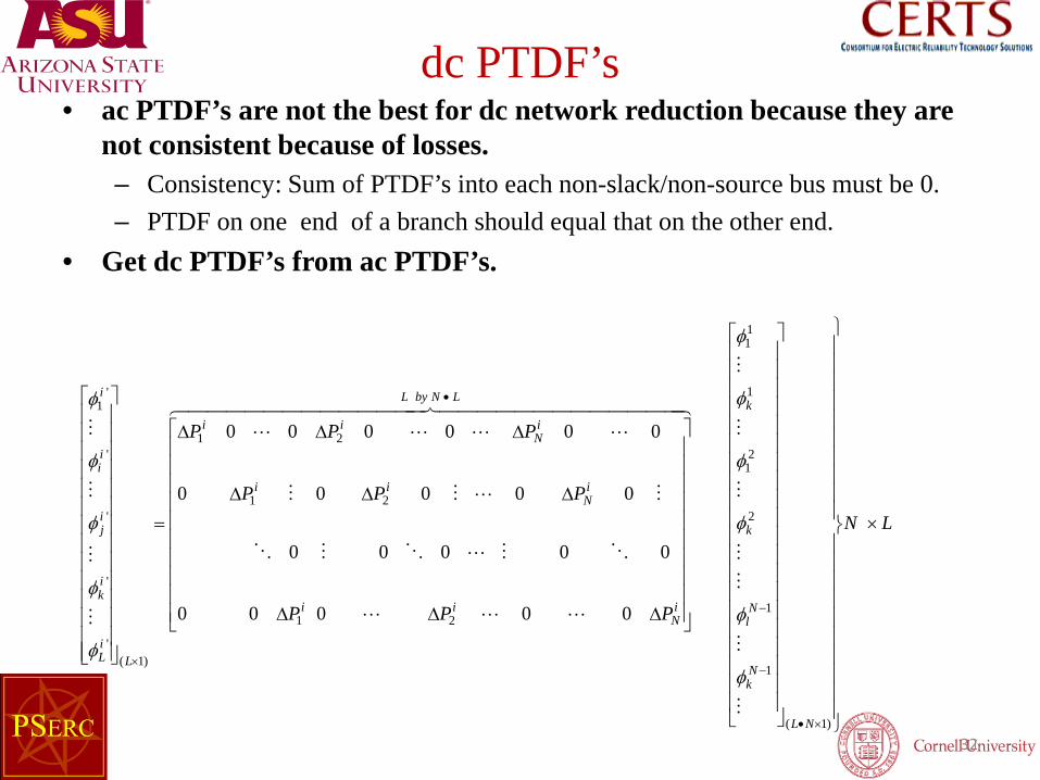
dc PTDF’s • ac PTDF’s are not the best for dc network reduction because they are
not consistent because of losses. – Consistency: Sum of PTDF’s into each non-slack/non-source bus must be 0. – PTDF on one end of a branch should equal that on the other end.
• Get dc PTDF’s from ac PTDF’s.
32
LN
PPP
PPP
PPP
NL
Nk
Nl
k
kLNbyL
iN
ii
iN
ii
iN
ii
LiL
ik
ij
ii
i
×
∆∆∆
∆∆∆
∆∆∆
=
ו
−
−
•
×
)1(
1
1
2
21
1
11
21
21
21
)1('
'
'
'
'1
00000
00000
00000
000000
φ
φ
φ
φ
φ
φ
φ
φ
φ
φ
φ
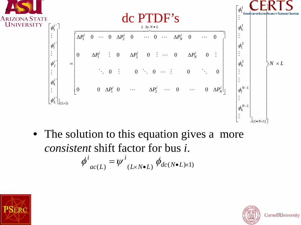
dc PTDF’s
• The solution to this equation gives a more consistent shift factor for bus i.
33
)1)()()( ו•×= LNdcLNL
iLac
i φψφ
acdc φψφ 1−=
LN
PPP
PPP
PPP
NL
Nk
Nl
k
kLNbyL
iN
ii
iN
ii
iN
ii
LiL
ik
ij
ii
i
×
∆∆∆
∆∆∆
∆∆∆
=
ו
−
−
•
×
)1(
1
1
2
21
1
11
21
21
21
)1('
'
'
'
'1
00000
00000
00000
000000
φ
φ
φ
φ
φ
φ
φ
φ
φ
φ
φ
1 1 1 11 1 2 3
11
2
1
212
2
2
1
2
(1 ) 0N
L
L
N
N
NL
P P P P− ∆ − ∆ − ∆ − ∆′ Φ
′Φ ′Φ
′Φ ′Φ
= ′Φ
′Φ ′Φ ′Φ
1 1 1 11 2 3
(1 )
00 0 0NP P P P− ∆ − ∆ − ∆ − ∆
0
1 1 1 11 2 3
2 2 2 21 2 3
(1 )
(1 )
00
N
N
P P P P
P P P P
− ∆ − ∆ − ∆ − ∆
−∆ − ∆ − ∆ − ∆
2 2 2 21 2 3
(1 )
00 0 0NP P P P− ∆ − ∆ − ∆ − ∆
0 0
2 2 2 21 2 3 (1 )
NP P P P− ∆ − ∆ − ∆ − ∆
1 2 3
N NP P P−∆ − ∆ − ∆
1 2 3
(1 )
(1
0 00
N NN
N N N
P
P P P
− ∆
− ∆ − ∆ − ∆ − ∆
)
0 0NNP
1 2 3 (1 )0 0 N N N NNP P P P
− ∆ − ∆ − ∆ − ∆
1121
11222
2
1
2
N
N
L
L
NL
Φ Φ
Φ Φ
Φ Φ
Φ
Φ Φ
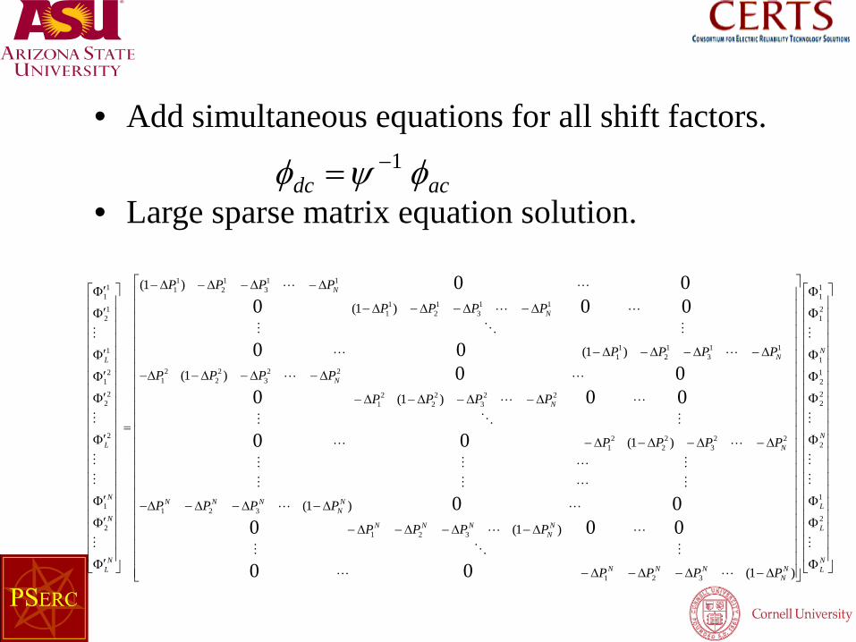
• Add simultaneous equations for all shift factors.
• Large sparse matrix equation solution.
acdc φψφ 1−=
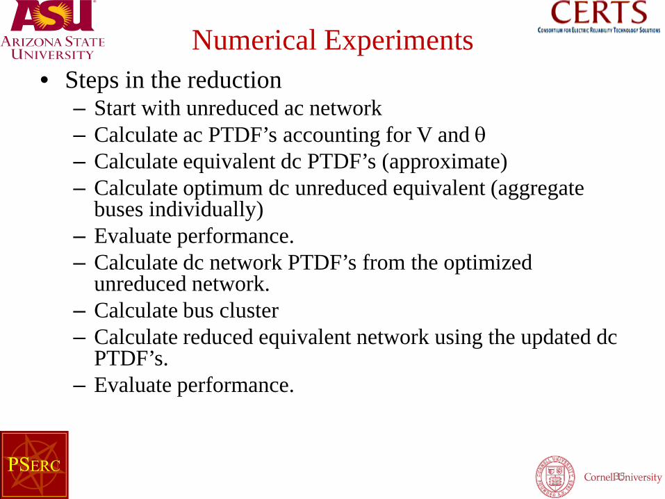
Numerical Experiments • Steps in the reduction
– Start with unreduced ac network – Calculate ac PTDF’s accounting for V and θ – Calculate equivalent dc PTDF’s (approximate) – Calculate optimum dc unreduced equivalent (aggregate
buses individually) – Evaluate performance. – Calculate dc network PTDF’s from the optimized
unreduced network. – Calculate bus cluster – Calculate reduced equivalent network using the updated dc
PTDF’s. – Evaluate performance.
35
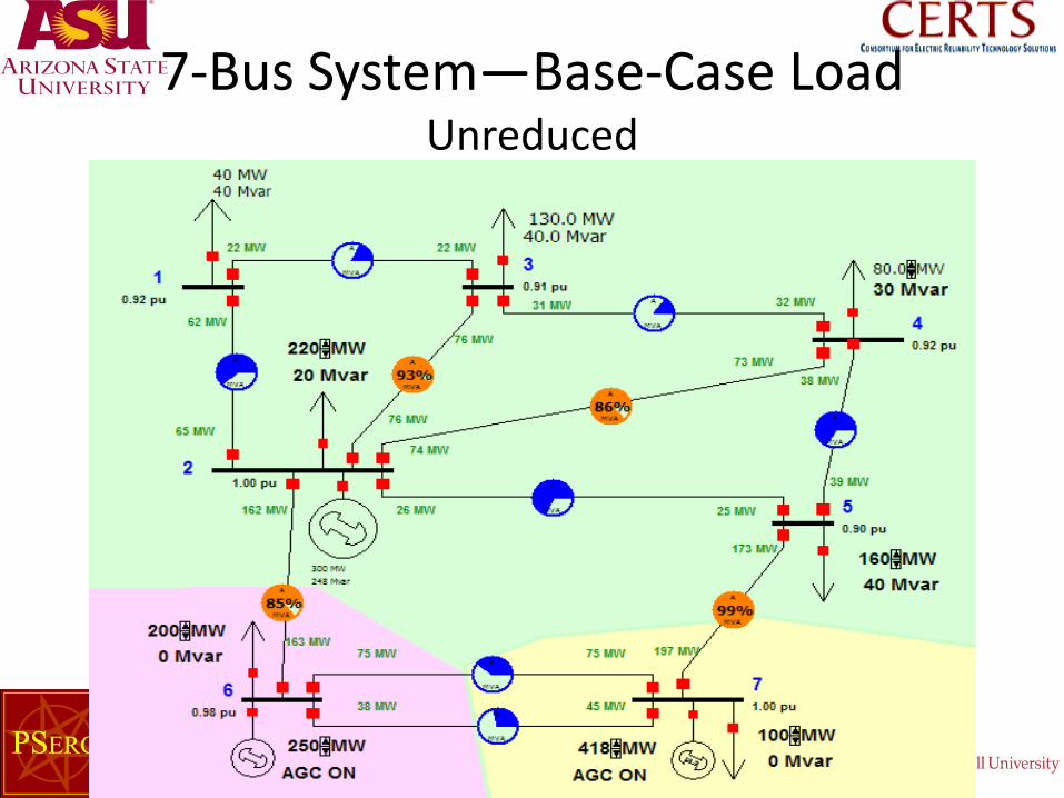
7-Bus System—Base-Case Load Unreduced
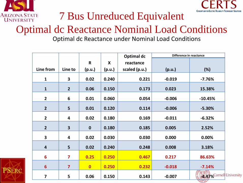
Line from Line to R
(p.u.) X
(p.u.)
Optimal dc reactance
scaled (p.u.)
Difference in reactance
(p.u.) (%)
1 3 0.02 0.240 0.221 -0.019 -7.76%
1 2 0.06 0.150 0.173 0.023 15.38%
2 6 0.01 0.060 0.054 -0.006 -10.45%
2 5 0.01 0.120 0.114 -0.006 -5.30%
2 4 0.02 0.180 0.169 -0.011 -6.32%
2 3 0 0.180 0.185 0.005 2.52%
3 4 0.02 0.030 0.030 0.000 0.00%
4 5 0.02 0.240 0.248 0.008 3.18%
6 7 0.25 0.250 0.467 0.217 86.63%
6 7 0 0.250 0.232 -0.018 -7.14%
7 5 0.06 0.150 0.143 -0.007 -4.47%
Optimal dc Reactance under Nominal Load Conditions
7 Bus Unreduced Equivalent Optimal dc Reactance Nominal Load Conditions
38
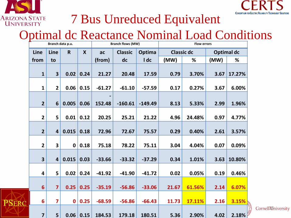
Branch data p.u. Branch flows (MW) Flow errors
Line from
Line to
R X ac (from)
Classic dc
Optimal dc
Classic dc Optimal dc (MW) % (MW) %
1 3 0.02 0.24 21.27 20.48 17.59 0.79 3.70% 3.67 17.27%
1 2 0.06 0.15 -61.27 -61.10 -57.59 0.17 0.27% 3.67 6.00%
2 6 0.005 0.06 -
152.48 -160.61 -149.49 8.13 5.33% 2.99 1.96%
2 5 0.01 0.12 20.25 25.21 21.22 4.96 24.48% 0.97 4.77%
2 4 0.015 0.18 72.96 72.67 75.57 0.29 0.40% 2.61 3.57%
2 3 0 0.18 75.18 78.22 75.11 3.04 4.04% 0.07 0.09%
3 4 0.015 0.03 -33.66 -33.32 -37.29 0.34 1.01% 3.63 10.80%
4 5 0.02 0.24 -41.92 -41.90 -41.72 0.02 0.05% 0.19 0.46%
6 7 0.25 0.25 -35.19 -56.86 -33.06 21.67 61.56% 2.14 6.07%
6 7 0 0.25 -68.59 -56.86 -66.43 11.73 17.11% 2.16 3.15%
7 5 0.06 0.15 184.53 179.18 180.51 5.36 2.90% 4.02 2.18%
7 Bus Unreduced Equivalent Optimal dc Reactance Nominal Load Conditions
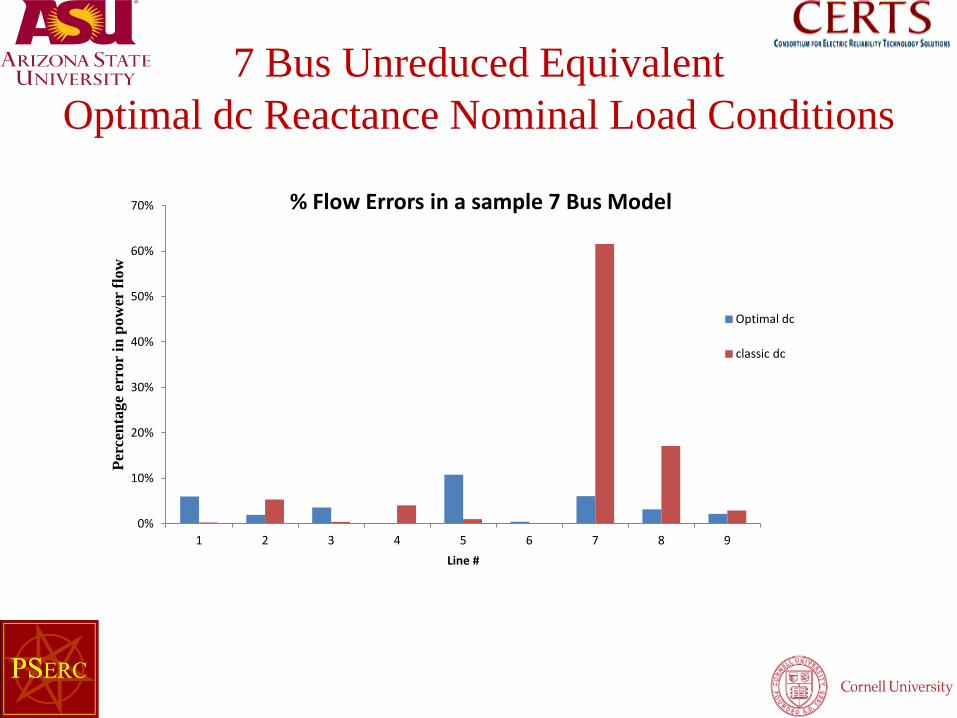
0%
10%
20%
30%
40%
50%
60%
70%
1 2 3 4 5 6 7 8 9
Perc
enta
ge e
rror
in p
ower
flow
Line #
% Flow Errors in a sample 7 Bus Model
Optimal dc
classic dc
7 Bus Unreduced Equivalent Optimal dc Reactance Nominal Load Conditions
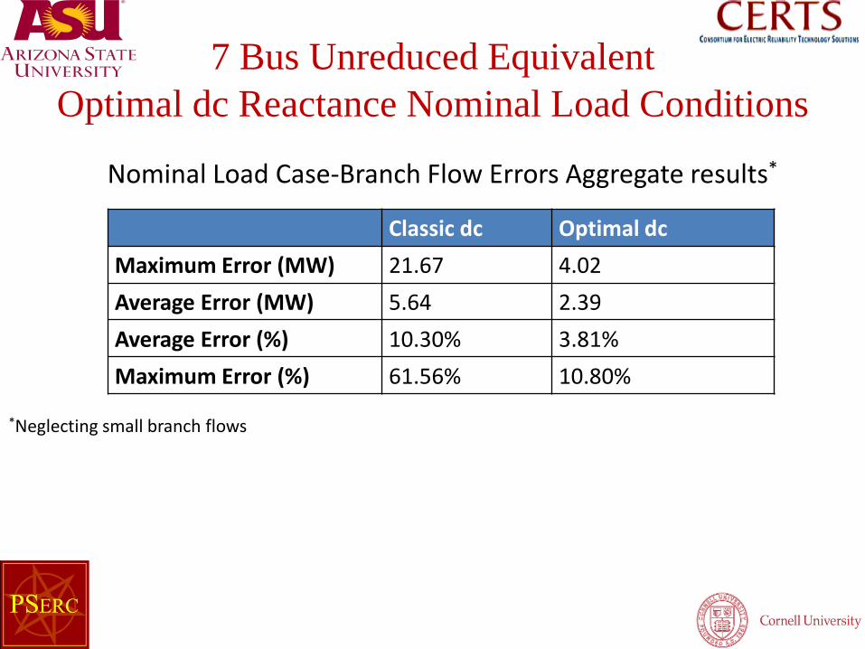
7 Bus Unreduced Equivalent Optimal dc Reactance Nominal Load Conditions
Classic dc Optimal dc Maximum Error (MW) 21.67 4.02 Average Error (MW) 5.64 2.39 Average Error (%) 10.30% 3.81% Maximum Error (%) 61.56% 10.80%
Nominal Load Case-Branch Flow Errors Aggregate results*
*Neglecting small branch flows

7 Bus Unreduced Equivalent Optimal dc Reactance Heavily Loaded Conditions
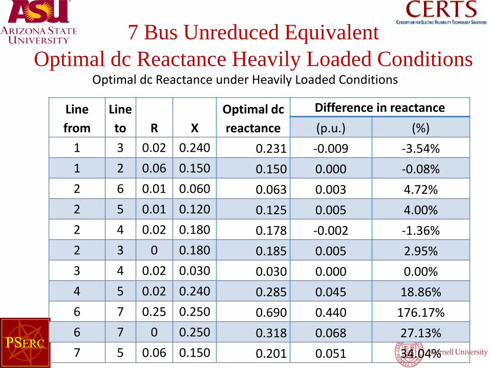
7 Bus Unreduced Equivalent Optimal dc Reactance Heavily Loaded Conditions
Line from
Line to R X
Optimal dc reactance
Difference in reactance (p.u.) (%)
1 3 0.02 0.240 0.231 -0.009 -3.54% 1 2 0.06 0.150 0.150 0.000 -0.08% 2 6 0.01 0.060 0.063 0.003 4.72% 2 5 0.01 0.120 0.125 0.005 4.00% 2 4 0.02 0.180 0.178 -0.002 -1.36% 2 3 0 0.180 0.185 0.005 2.95% 3 4 0.02 0.030 0.030 0.000 0.00% 4 5 0.02 0.240 0.285 0.045 18.86% 6 7 0.25 0.250 0.690 0.440 176.17% 6 7 0 0.250 0.318 0.068 27.13% 7 5 0.06 0.150 0.201 0.051 34.04%
Optimal dc Reactance under Heavily Loaded Conditions
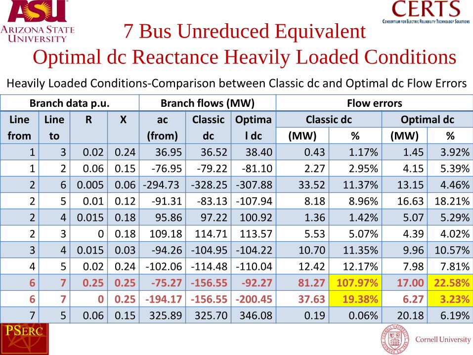
Branch data p.u. Branch flows (MW) Flow errors Line from
Line to
R X ac (from)
Classic dc
Optimal dc
Classic dc Optimal dc (MW) % (MW) %
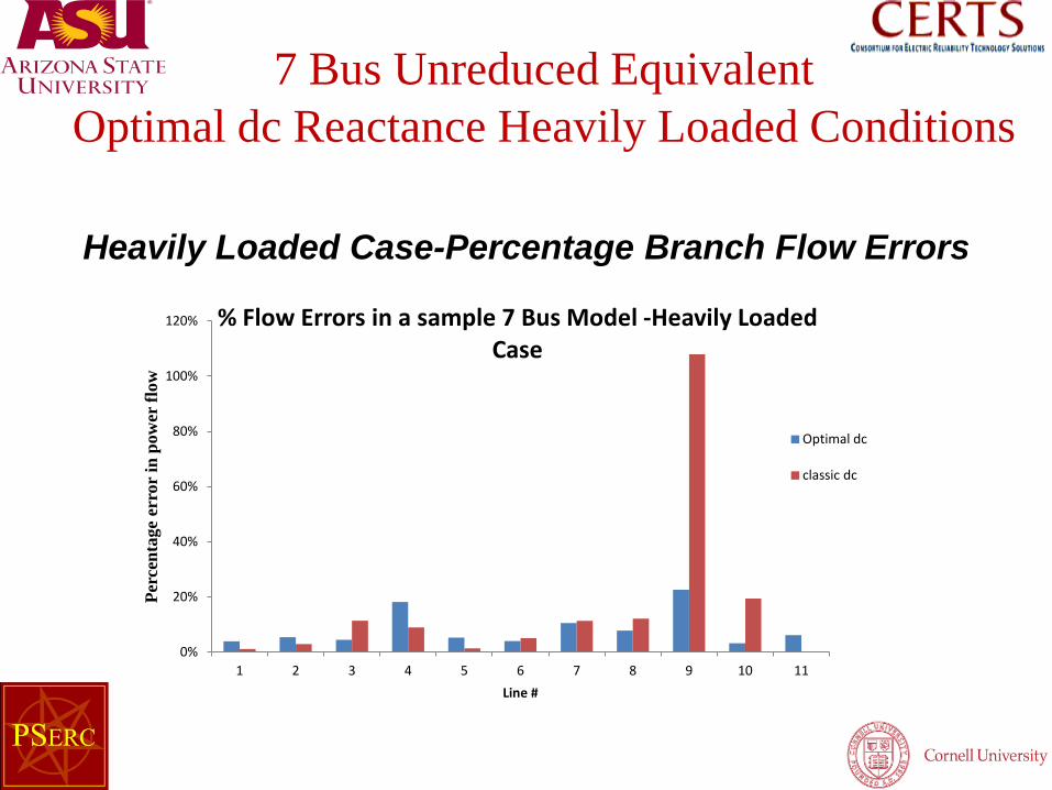
1 3 0.02 0.24 36.95 36.52 38.40 0.43 1.17% 1.45 3.92% 1 2 0.06 0.15 -76.95 -79.22 -81.10 2.27 2.95% 4.15 5.39% 2 6 0.005 0.06 -294.73 -328.25 -307.88 33.52 11.37% 13.15 4.46% 2 5 0.01 0.12 -91.31 -83.13 -107.94 8.18 8.96% 16.63 18.21% 2 4 0.015 0.18 95.86 97.22 100.92 1.36 1.42% 5.07 5.29% 2 3 0 0.18 109.18 114.71 113.57 5.53 5.07% 4.39 4.02% 3 4 0.015 0.03 -94.26 -104.95 -104.22 10.70 11.35% 9.96 10.57% 4 5 0.02 0.24 -102.06 -114.48 -110.04 12.42 12.17% 7.98 7.81% 6 7 0.25 0.25 -75.27 -156.55 -92.27 81.27 107.97% 17.00 22.58% 6 7 0 0.25 -194.17 -156.55 -200.45 37.63 19.38% 6.27 3.23% 7 5 0.06 0.15 325.89 325.70 346.08 0.19 0.06% 20.18 6.19%
7 Bus Unreduced Equivalent Optimal dc Reactance Heavily Loaded Conditions
Heavily Loaded Conditions-Comparison between Classic dc and Optimal dc Flow Errors
7 Bus Unreduced Equivalent Optimal dc Reactance Heavily Loaded Conditions
0%
20%
40%
60%
80%
100%
120%
1 2 3 4 5 6 7 8 9 10 11
Perc
enta
ge e
rror
in p
ower
flow
Line #
% Flow Errors in a sample 7 Bus Model -Heavily Loaded Case
Optimal dc
classic dc
Heavily Loaded Case-Percentage Branch Flow Errors
7 Bus Unreduced Equivalent Optimal dc Reactance Heavily Loaded Conditions
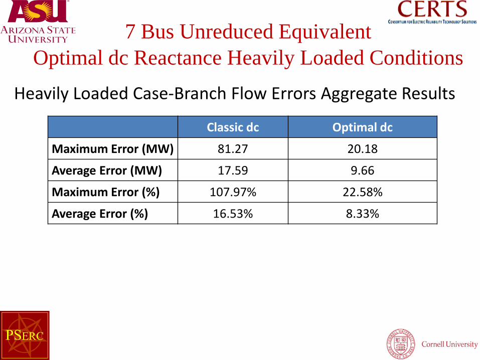
Classic dc Optimal dc
Maximum Error (MW) 81.27 20.18
Average Error (MW) 17.59 9.66
Maximum Error (%) 107.97% 22.58%
Average Error (%) 16.53% 8.33%
Heavily Loaded Case-Branch Flow Errors Aggregate Results
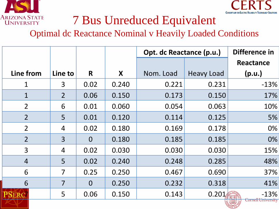
7 Bus Unreduced Equivalent Optimal dc Reactance Nominal v Heavily Loaded Conditions
Line from Line to R X
Opt. dc Reactance (p.u.) Difference in Reactance
(p.u.) Nom. Load Heavy Load 1 3 0.02 0.240 0.221 0.231 -13% 1 2 0.06 0.150 0.173 0.150 17% 2 6 0.01 0.060 0.054 0.063 10% 2 5 0.01 0.120 0.114 0.125 5% 2 4 0.02 0.180 0.169 0.178 0% 2 3 0 0.180 0.185 0.185 0% 3 4 0.02 0.030 0.030 0.030 15% 4 5 0.02 0.240 0.248 0.285 48% 6 7 0.25 0.250 0.467 0.690 37% 6 7 0 0.250 0.232 0.318 41% 7 5 0.06 0.150 0.143 0.201 -13%
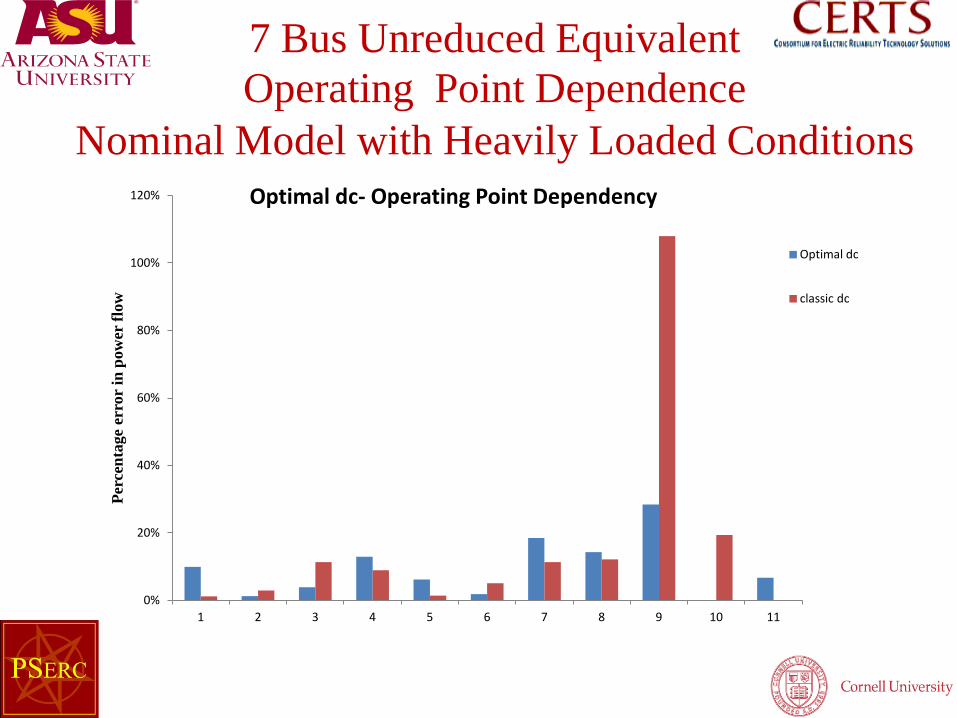
7 Bus Unreduced Equivalent Operating Point Dependence
Nominal Model with Heavily Loaded Conditions
0%
20%
40%
60%
80%
100%
120%
1 2 3 4 5 6 7 8 9 10 11
Perc
enta
ge e
rror
in p
ower
flow
Optimal dc- Operating Point Dependency
Optimal dc
classic dc
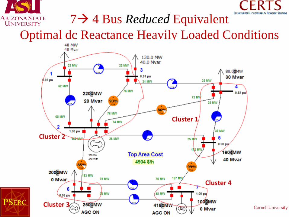
7 4 Bus Reduced Equivalent Optimal dc Reactance Heavily Loaded Conditions
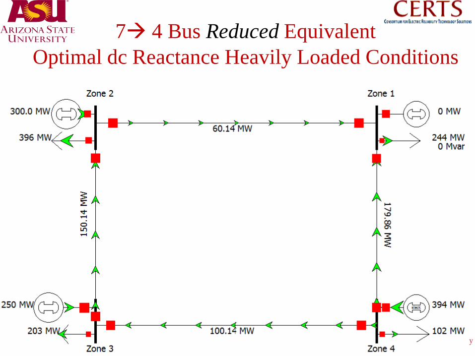
7 4 Bus Reduced Equivalent Optimal dc Reactance Heavily Loaded Conditions
7 4 Bus Reduced Equivalent Optimal dc Reactance Heavily Loaded Conditions
Branch data p.u.
Branch flows (MW) Flow errors
Line from
Line to
ac (from)
Classic dc
Optimal dc Classic dc Optimal dc (MW) % (MW) %
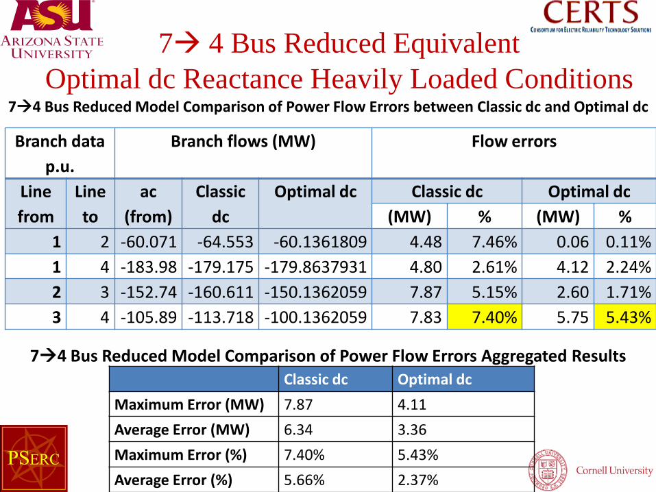
1 2 -60.071 -64.553 -60.1361809 4.48 7.46% 0.06 0.11% 1 4 -183.98 -179.175 -179.8637931 4.80 2.61% 4.12 2.24% 2 3 -152.74 -160.611 -150.1362059 7.87 5.15% 2.60 1.71% 3 4 -105.89 -113.718 -100.1362059 7.83 7.40% 5.75 5.43%
74 Bus Reduced Model Comparison of Power Flow Errors between Classic dc and Optimal dc
Classic dc Optimal dc Maximum Error (MW) 7.87 4.11 Average Error (MW) 6.34 3.36 Maximum Error (%) 7.40% 5.43% Average Error (%) 5.66% 2.37%
74 Bus Reduced Model Comparison of Power Flow Errors Aggregated Results
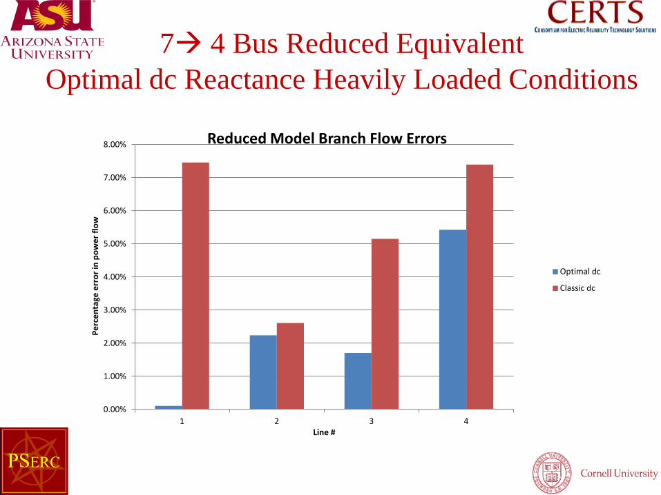
7 4 Bus Reduced Equivalent Optimal dc Reactance Heavily Loaded Conditions
0.00%
1.00%
2.00%
3.00%
4.00%
5.00%
6.00%
7.00%
8.00%
1 2 3 4
Per
cent
age
erro
r in
pow
er fl
ow
Line #
Reduced Model Branch Flow Errors
Optimal dc
Classic dc
• 118 bus network example (IEEE network) – Classical dc model – Optimum dc model – Flow errors
52
IEEE 18-Bus Unreduced Equivalent
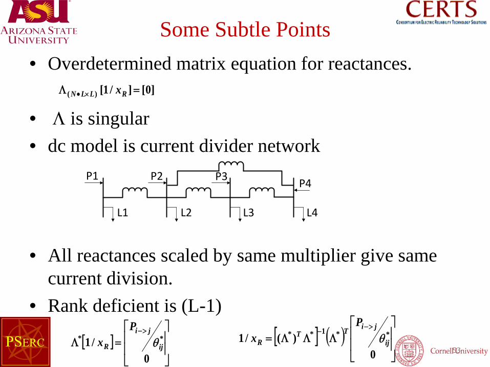
Some Subtle Points • Overdetermined matrix equation for reactances.
• Λ is singular • dc model is current divider network
• All reactances scaled by same multiplier give same current division.
• Rank deficient is (L-1)
53 [ ] ( )
ΛΛΛ=
>−−
0)(/1 **1**
ij
jiTTR
Px θ
]0[]/1[)( =Λ ×• RLLN x
[ ]
=Λ
>−
0/1 **
ij
ji
R
Px θ
L1 L2 L3 L4
P4P3P2P1
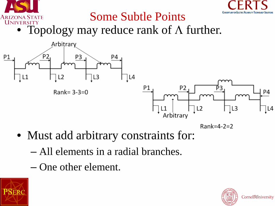
Some Subtle Points • Topology may reduce rank of Λ further.
• Must add arbitrary constraints for: – All elements in a radial branches. – One other element.
54
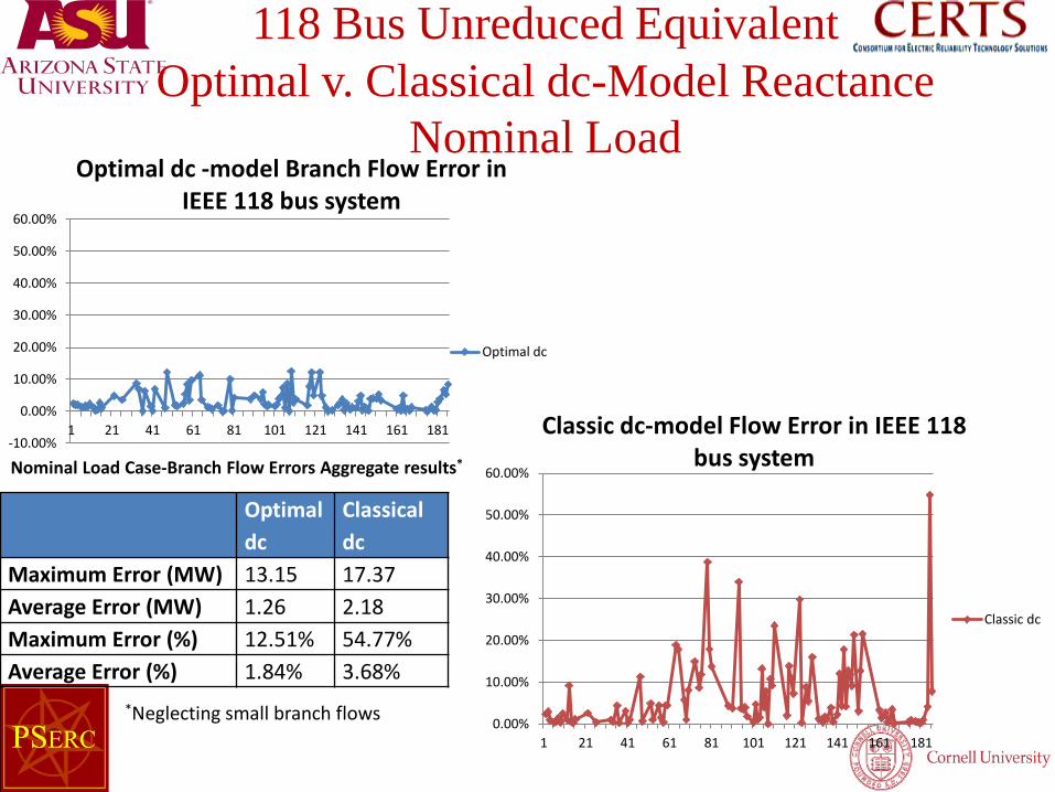
118 Bus Unreduced Equivalent Optimal v. Classical dc-Model Reactance
Nominal Load
-10.00%
0.00%
10.00%
20.00%
30.00%
40.00%
50.00%
60.00%
1 21 41 61 81 101 121 141 161 181
Optimal dc -model Branch Flow Error in IEEE 118 bus system
Optimal dc
0.00%
10.00%
20.00%
30.00%
40.00%
50.00%
60.00%
1 21 41 61 81 101 121 141 161 181
Classic dc-model Flow Error in IEEE 118 bus system
Classic dc
Optimal dc
Classical dc
Maximum Error (MW) 13.15 17.37 Average Error (MW) 1.26 2.18 Maximum Error (%) 12.51% 54.77% Average Error (%) 1.84% 3.68%
Nominal Load Case-Branch Flow Errors Aggregate results*
*Neglecting small branch flows
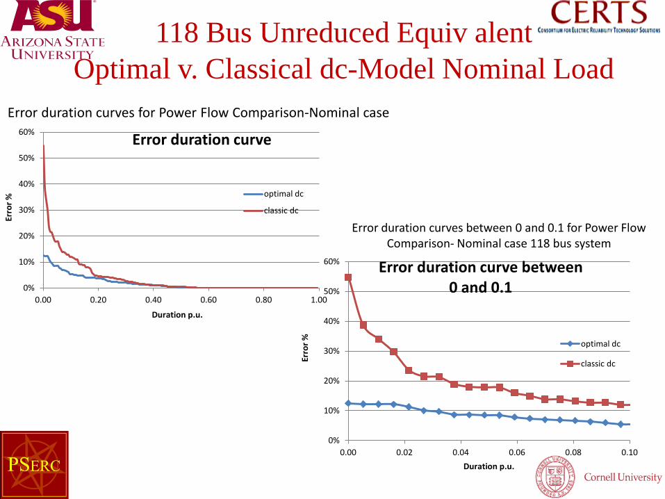
118 Bus Unreduced Equiv alent Optimal v. Classical dc-Model Nominal Load
0%
10%
20%
30%
40%
50%
60%
0.00 0.20 0.40 0.60 0.80 1.00
Erro
r %
Duration p.u.
Error duration curve
optimal dc
classic dc
Error duration curves for Power Flow Comparison-Nominal case
0%
10%
20%
30%
40%
50%
60%
0.00 0.02 0.04 0.06 0.08 0.10
Erro
r %
Duration p.u.
Error duration curve between 0 and 0.1
optimal dc
classic dc
Error duration curves between 0 and 0.1 for Power Flow Comparison- Nominal case 118 bus system
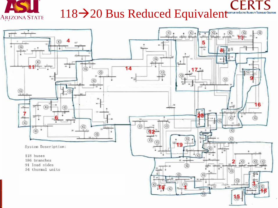
11820 Bus Reduced Equivalent Optimal v. Classical dc-Model Nominal Load
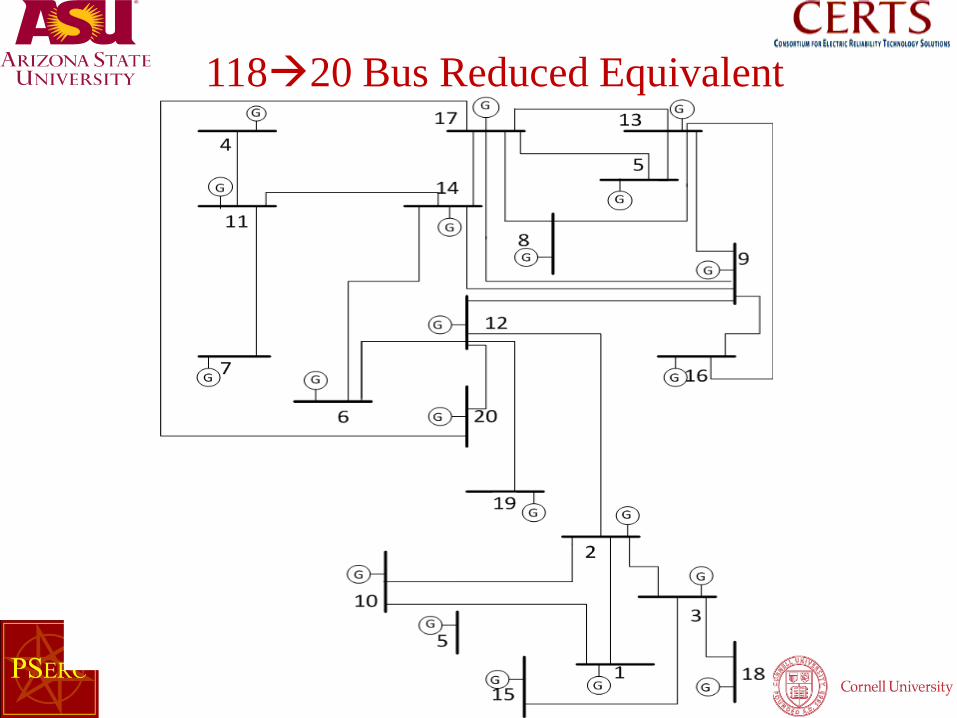
11820 Bus Reduced Equivalent
11820 Bus Reduced Equivalent Optimal v. Classical dc-Model Nominal Load
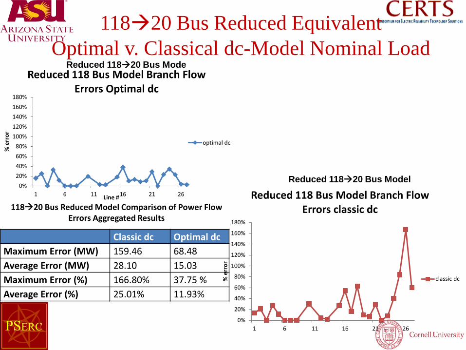
0% 20% 40% 60% 80%
100% 120% 140% 160% 180%
1 6 11 16 21 26
% e
rror
Line #
Reduced 118 Bus Model Branch Flow Errors Optimal dc
optimal dc
Reduced 11820 Bus Mode
0%
20%
40%
60%
80%
100%
120%
140%
160%
180%
1 6 11 16 21 26
% e
rror
Reduced 118 Bus Model Branch Flow Errors classic dc
classic dc
Reduced 11820 Bus Model
Classic dc Optimal dc Maximum Error (MW) 159.46 68.48 Average Error (MW) 28.10 15.03 Maximum Error (%) 166.80% 37.75 % Average Error (%) 25.01% 11.93%
11820 Bus Reduced Model Comparison of Power Flow Errors Aggregated Results
Conclusions
• For bus aggregation based network equivalencing it was found that: – By reducing small elements in the Λ matrix:
• Significant speed up in computation time. • Problem size may be reduced to fit on a PC
– By calculation optimum branch reactance evaluation: • Unreduced dc network flows errors are significantly decreased. • Reduced of flow errors in the reduced network equivalent are also
significantly decreased.
60

Questions?