Economic growth theory

1 Introduction and empirical facts

• in discrete time, x(t+ s) = x(t)(1 + γx)s ( =⇒ compute average growth rate)

• in continuous time, x(t+ s) = x(t)eγxs. Further:

– γxy(t) = γx(t) + γy(t)

– γx/y(t) = γx(t)− γy(t)

– γxα(t) = αγx(t)

– γx(t) = β (constant) ⇔ x(t) = Beβt

– In a diagram with lnx(t) over t:

I If x(t) grows at constant rate β, lnx(t) shows up as a line with slope β.

I If both x(t) and z(t) grow at the same (constant) rate, then lnx(t)− ln z(t) remains constant=⇒ the graphs are parallel lines.

• Balanced growth: Most economies typically exhibit balanced growth, i.e. they seem to follow agrowth path along which the following variables are roughly constant:

– the growth rates of real per-capita GDP, real per-capita consumption, and the per-capita capitalstock

– the real interest rate

– the income shares of capital and labor

2 Basic assumptions, growth accounting

• Central assumptions:

– Relative prices are flexible and all markets clear at all times.

– Money is neutral and monetary variables can therefore be omitted from growth models.

• Aggregate production function: Y (t) = F (K(t), L(t), A(t))

• Aggregate model: a single output good is produced from two input factors (capital and labor) with agiven technology

• changes in A(t) are interpreted as technological progress (or decline)

• Further assumptions

– F (increasing, convave in K,L) is twice continuously differentiable in K,L

– Positive marginal products of capital and labor: F1(K,L, A) > 0, F2(K,L, A) > 0

– Diminishing marginal products (diminishing returns) of capital and labor: F11(K,L, A) < 0, F22(K,L, A) <0

– constant returns to scale (linear homogeneity) with respect to capital and labor: ∀λ > 0,∀(K,L, A) ∈R3

+, F (λK, λL, A) = λF (K,L, A) (no learning effects, no ”crowding” effects)

• Factor prices under perfect competition (no monopolies, households and firms take price as given)

– w(t) denotes real wage at time t, q(t) denotes real rental price of capital at time t (expressed inunits of period-t output)

1

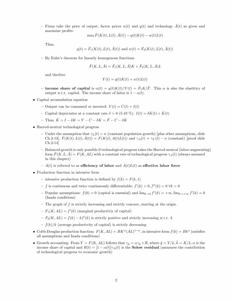
– Firms take the price of output, factor prices w(t) and q(t) and technology A(t) as given andmaximize profits:

max F (K(t), L(t), A(t))− q(t)K(t)− w(t)L(t)

Thus,q(t) = F1(K(t), L(t), A(t)) and w(t) = F2(K(t), L(t), A(t))

– By Euler’s theorem for linearly homogenous functions

F (K,L, A) = F1(K,L, A)K + F2(K,L, A)L

and therforeY (t) = q(t)K(t) + w(t)L(t)

– income share of capital is α(t) = q(t)K(t)/Y (t) = F1K/F . This α is also the elastiticy ofoutput w.r.t. capital. The income share of labor is 1− α(t).

• Capital accumulation equation

– Output can be consumed or invested: Y (t) = C(t) + I(t)

– Capital depreciates at a constant rate δ > 0 (5-10 %). I(t) = δK(t) + K(t)

– Thus, K = I − δK = Y − C − δK = F − C − δK

• Harrod-neutral technological progress

– Under the assumption that γL(t) = n (constant population growth) [plus other assumptions, slideCh.2-13], F (K(t), L(t), A(t)) = F (K(t), A(t)L(t)) and γA(t) = γY (t) − n (constant) [proof slideCh.2-14]

– Balanced growth is only possible if technological progress takes the Harrod-neutral (labor-augmenting)form F (K,L, A) = F (K,AL) with a constant rate of technological progress γA(t) (always assumedin this chapter)

– A(t) is referred to as efficiency of labor and A(t)L(t) as effective labor force

• Production function in intensive form

– intensive production function is defined by f(k) = F (k, 1)

– f is continuous and twice continuously differentiable; f ′(k) > 0, f ′′(k) < 0 ∀k > 0

– Popular assumptions: f(0) = 0 (capital is essential) and limk→0 f′(k) = +∞, limk→+∞ f ′(k) = 0

(Inada conditions)

– The graph of f is strictly increasing and strictly concave, starting at the origin.

– F1(K,AL) = f ′(k) (marginal productiviy of capital)

– F2(K,AL) = f(k)− kf ′(k) is strictly positive and strictly increasing w.r.t. k

– f(k)/k (average productivity of capital) is strictly decreasing

• Cobb-Douglas production function: F (K,AL) = BKα(AL)1−α, in intensive form f(k) = Bkα (satisfiesall assumptions and Inada conditions)

• Growth accounting: From Y = F (K,AL) follows that γy = αγk+R, where y = Y/L, k = K/L,α is theincome share of capital and R(t) = [1− α(t)]γA(t) is the Solow residual (measures the contributionof technological progress to economic growth)

2

3 The simplest neoclassical growth model (Solow-Swan model)

• Aggregate model; closed economy; exogenous population growth; exogenous technological progress;exogenous saving rate (no optimization)

Y (t) = F (K(t), A(t)L(t))

A(t) = gA(t), A(0) = A0

L(t) = nL(t), L(0) = L0

Y (t) = C(t) + I(t)

I(t) = δK(t) + K(t) = sY (t),K(0) = K0

• Results

– A = A0egt, L = L0e

nt

– k = K/(AL) (capital stock per unit of effective labor)

– k = sf(k)− (n+ δ + g)k

– limt→+∞ = k∗, where k∗ is determined uniquely by sf(k∗) = (n + δ + g)k∗ and is called a fixedpoint or steady state

• Balanced growth path (all variables grow at constant rate)

K = kAL = A0L0k∗e(n+g)t

Y = f(k)AL = A0L0f(k∗)e(n+g)t

k = K/L = A0k∗egt

y = Y/L = A0f(k∗)egt

c = C/L = (1− s)A0f(k∗)egt

• Long-run growth rate: limt→+∞ γy(t) = g (the only exogenous variable that affects the long-run growthrate is the rate of technological progress g)

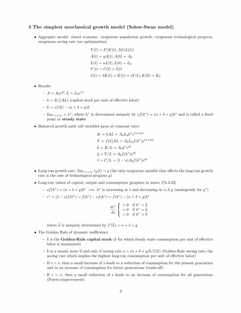
• Long-run values of capital, output and consumption [graphics in notes, Ch.3-23]

– sf(k∗) = (n+ δ + g)k∗ =⇒ k∗ is increasing in s and decreasing in n, δ, g (analogously for y∗)

– c∗ = (1− s)f(k∗) = f(k∗)− sf(k∗) = f(k∗)− (n+ δ + g)k∗

dc∗

ds

> 0 if k∗ < k= 0 if k∗ = k< 0 if k∗ > k

where k is uniquely determined by f ′(k) = n+ δ + g

• The Golden Rule of dynamic inefficiency

– k is the Golden-Rule capital stock (k for which steady state consumption per unit of effectivelabor is maximized)

– k is a steady state if and only if saving rate s = (n+ δ + g)k/f(k) (Golden-Rule saving rate; thesaving rate which implies the highest long-run consumption per unit of effective labor)

– If s < s, then a small increase of s leads to a reduction of consumption for the present generationand to an increase of consumption for future generations (trade-off)

– If s > s, then a small reduction of s leads to an increase of consumption for all generations(Pareto-improvement)

3

– A saving rate s > s is called dynamically inefficient (capital overaccumulation)

– Empirically, typically s < s

• The Cobb-Douglas case

– F (K,AL) = BKα(AL)1−α =⇒ k(t) = sBk(t)α − (n+ δ + g)k(t)

– Steady state (where k = 0) can be computed explicitly [Ch.3-25]

• Transition dynamics in the general case [Ch.3-26]: a first-order approximation for the rate of conver-gence close to the fixed point k∗ is given by λ = (1− α∗)(n+ δ + g)

• Major predictions of the Solow-Swan model

– Technological progress is necessary for long-run growth. Capital accumulation alone cannot sus-tain growth due to diminishing returns to capital.

– The model predicts conditional convergence of growth rates and per-capita income levels (if tech-nological progress is the same in two countries, also their long-run growth rates should be thesame; if additionally their f, n + δ + g are the same, then also their long-run per-capita incomelevels should be the same)

• Elasticity of long-run output level w.r.t. the saving rate is sy∗

∂y∗

∂s = α∗

1−α∗ . Along a balanced growth

path, also the elasticity of per-capita GDP w.r.t. the saving rate is α∗

1−α∗ , which would result in anunreasonably small dispersion among countries.

4 Cross-country income differences and convergence

• absolute β convergence: ”Poorer” country grows faster unconditionally (only supported for ”similar”countries like OECD countries; not supported by empirical evidence if the cross-section of countries issufficiently broad, Ch.4-31).

• conditional β convergence: ”Poorer” country grows faster only if it is farther away from its balancedgrowth path.

• σ convergence: The dispersion of per-capita income levels across countries relative to the averageincome level declines over time (coefficient of variation).

5 Traditional neoclassical growth theories

(a) Infinitely-lived households (Ramsey-Cass-Koopmans model)

• Dynamic general-equilibrium model: goods market, labor market, capital market

• Walrasian model: perfect competition, rational expectations (perfect foresight), complete markets

• Explicit micro foundations: firms maximize profits, households maximize utility; households own thefactors of production; welfare analysis is possible

• The saving rate is endogenously determined as part of the solution of the households’ optimizationproblem

• Firms

– Unit interval of identical firms (aggregate output, employment etc. equals output, employmentetc. of the representative firm)

– The representative firm produces output at time t according to the production function Y (t) =F (K(t), A(t)L(t))

4

– The firm takes capital rent q(t), real wage rent w(t) and the state of technology A(t) as givenand maximizes profits w.r.t. Y (t),K(t) and L(t) (static optimization in each period; NO dynamicoptimization).

– FOC: q(t) = F1(K,AL), w(t) = AF2(K,AL)

– y = Y/(AL), k = K/(AL) =⇒ conditions in intensive form:

y(t) = f(k(t))

q(t) = f ′(k(t)) marginal productivity of capital

w(t) = A(t)[f(k(t))− k(t)f ′(k(t))]

• Technology: A = gA(t), capital depreciates at constant rate δ =⇒ return to capital (real interestrate) r(t) = q(t)− δ

• The lifetime budget constraint of the households

– H identical and infinitely-lived households (dynasties), each growing at constant rate n. Popula-tion size (labor force) L satisfies L = nL

– Every member of households is endowed with one unit of time to work =⇒ labor supply of singlehousehold is L(t)/H

– Every household owns at time t capital stock K(t)/H, where K(0) is a given constant.

– Every individual consumes at time t the amount c(t) = C(t)/L(t), i.e. every household consumesC(t)/H

– Lifetime budget constraint: the present value of a household’s consumption between time 0 and+∞ must not exceed the present value of its endowment with capital and total wage income:∫ +∞

t=0

e−R(t)C(t)/Hdt ≤ K(0)/H +

∫ +∞

t=0

e−R(t)w(t)L(t)/Hdt

where the first term is the discount factor, the second the consumption expenditure in t, the thirdthe initial endowment, and the forth the present value of wage income of the entire lifetime.

Capital income is included in R:

R(t) =

∫ t

0

r(τ)dτ

• Present value of capital stock at time T is

e−R(T )K(T ) = K(0) +

∫ T

t=0

e−R(t)[w(t)L(t)− C(t)]dt

which upon differentiation w.r.t T , multiplying by eR(t) and using R(T ) = r(T ) yields

K(t) = w(t)L(t) + r(t)K(t)− C(t)

• Transversality condition: limt→+∞ e−R(t)K(t) = 0 (at the end of time, no capital should be left back)

• In per-capita variables,˙k = w(t) + [r(t)− n]k(t)− c(t)

• In intensive variables, k = w(t)/A(t) + [r(t)− (n+ g)]k(t)− c(t)

• Households maximize∫ +∞t=0

= e−ρtU(c(t))L(t)/Hdt, where ρ measures relative weight given to futureconsumption (high ρ corresponds with high impatience)

5

• As γL(t) = n, the objective function can be rewritten as∫ +∞t=0

e−(ρ−n)tU(c(t))dt

• So, the households maximizes ∫ +∞

t=0

e−(ρ−n)tU(c(t))dt

subject to

˙k = w(t) + [r(t)− n]k(t)− c(t)

limt→+∞

e−R(t)entk(t) ≥ 0

c(t) ≥ 0

choosing k(t), c(t) and w(t), r(t) given

• Euler equation [Ch.5a-41, notes]: γc =˙c(t)c(t) = r(t)−ρ

εU (c(t)) , where εU is the elasticity of the marginal utility

at c or the inverse of the elasticity of intertemporal substitution: εU (c) = −U′′(c)cU ′(c) > 0

• If r(t) > ρ, it pays to postpone consumption, i.e., current per-capita consumption must be smallerthan future consumption (γc > 0)

• If ρ > r(t), the household is very impatient and saves only little =⇒ present per-capita householdmust be higher than future consumption (γc < 0)

• These effects are strong, if the elasticity of intertemporal substitution is large

• Balanced growth and the elasticity of substitution: By the Euler equation, there is only aconstant growth rate (balanced growth path) of per-capita consumption if depending on the constantreal interest rate there exists a constant θ > 0 s.t. εU (c) = θ holds for all c ≥ 0. Thus

U(c) =

{c1−θ−1

1−θ if θ 6= 1

ln(c) if θ = 1

where θ determines the curvature of the utility function. The higher the curvature, the stronger isthe desire of the household to have a smooth consumption stream =⇒ θ determines how strongly ahousehold reacts to intertemporal price differences. The elasticity of intertemporal substitutionis equal to 1/θ.

• Equilibrium

Firms:

r(t) = f ′(k(t))− δw(t) = A(t)[f(k(t))− k(t)f ′(k(t))]

Households:

k(t) = w(t)/A(t)− [r(t)− n− g]k(t)− c(t)c(t) = c(t)[r(t)− ρ− θg]/θ from Euler equation

k(0) = k0 = K(0)/[A(0)L(0)]

limt→+∞

e−R(t)e(n+g)tk(t) = 0

Equilibrium:

k(t) = f(k(t))− (n+ g + δ)k(t)− c(t)c(t) = c(t)[f ′(k(t))− ρ− δ − θg]/θ

6

subject to boundary conditions:

k(0) = k0

limt→+∞

e−R(t)e(n+g)tk(t) = 0

• Phase diagram analysis [Ch.5a-45, notes]

– The isocline c(t) = 0 consists of the two lines c = 0 and k = k∗, where k∗ is determined byf ′(k∗) = ρ+ δ + θg (so c(t) grows to the left of this line, and falls to its right)

– The isocline k(t) = 0 is the curve c = f(k)− (n+ δ+ g)k (so k(t) grows below this curve and fallsabove it)

– The isocline k(t) = 0 attains its maximum at k = k, where k is the Golden-rule capital stock.Generally, k∗ < k

– Three fixed points of the system of two differential equations: (0, 0), (k∗, c∗), (k, 0)

• Stable saddle point path

– In equilibrium, the differential for k(t) and c(t) and the initial and transversality conditions mustbe satisfied.

– If c(0) large, k(t) becomes negative, so this cannot be a solution

– If c(0) small, solutions converge to (k, 0), in which case the transversality condition would beviolated, so this cannot be a stable saddle point path either.

– Only for one unique value c(0) the solutions remain feasible and satisfy initial and transversalityconditions. This solution converges to (k∗, c∗) (increasing curve in (k, c) diagram)

• Balanced growth path

– As k(t)→ k∗, it follows that y(t)→ y∗ = f(k∗) and c(t)→ c∗ = f(k∗)− (n+ δ + g)k∗

– As in the Solow-Swan model, all equilibria converge to a balanced growth path

K = kAL = A0L0k∗e(n+g)t

Y = f(k)AL = A0L0f(k∗)e(n+g)t

k = K/L = A0k∗egt

y = Y/L = A0f(k∗)egt

c = C/L = A0[f(k∗)− (n+ δ + g)k∗]egt

– The long-run growth rate is g. No other parameter has a long-run growth effect.

– k∗ is a decreasing function of ρ, δ, θ and g, and is independent of n

– c∗ is a decreasing function of ρ, δ, θ, g, n.

• Transition dynamics - non-anticipated parameter change at time t0 [notes]

– Before t0, the equilibrium is described by the old stable saddle point path. Immediately beforet0, the economy is in state (k(t−0 ), c(t−0 )).

– There is a new stable saddle point path corresponding to the new parameters.

– After t0, the equilibrium follows the new saddle point path starting in k(t0) = k(t−0 )

• Transition dynamics - parameter change at time t1 that becomes already known at time t0 (an-nouncement effect)

7

– Before t0 the equilibrium is described by the old stable saddle point path. Immediately before t0,the economy is in state (k(t−0 ), c(t−0 )).

– There is a new stable saddle point path corresponding to the new parameters.

– After t1 the equilibrium follow the new saddle point path.

– Between t0 and t1, the equilibrium is characterized by that solution of the old phase diagram,which leads from k(t0) = k(t−0 ) in exactly t1 − t0 time units to the new stable saddle point path.

• Adjustment speed: Linearization around the fixed point [Ch.5a-49; notes] with some reasonableparameters yields λ1 = −12.1%, λ2 = 15.1% (which can be disregarded on economic grounds?), i.e.,within 6 years the distance between k(t) and k∗ is reduced by 50% (faster convergence than in theSolow model).

• For g = 0, dλ1/dθ > 0, i.e. higher elasticity of intertemporal substitution leads to higher adjustmentspeed.

• Pareto-efficiency: A social planner has to obey technological constraints and economy-wide resourceconstraints, but is not subject to budget constraints. His FOC are identical to decentralized economy.Thus, the market equilibrium obtained before is Pareto-efficient (because there is a ”perfect” market,and everybody is perfectly rational). The First Welfare Theorem applies, i.e., there is no role forthe government in this model.

(b) Overlapping generations of finitely-lived households (Diamond model)

• Similarities to Ramsey-Cass-Koopmans model:

– Households and firms interact on the markets for goods, capital, labor (dynamic general equilib-rium model).

– Perfect competition, complete markets, perfect foresight (Walrasian model).

– Saving rate endogenously determined by the households’ utility maximization problem.

• Main differences to Ramsey-Cass-Koopmans model:

– Households have finite lifetimes, but there are infinitely many overlapping generations of house-holds.

– The structure of the equilibrium set and the equilibrium dynamics can be more complicated

– Equilibria need not be Pareto-efficient (First Welfare Theorem fails!)

– Technical assumption: Discrete time periods. Every household lives for two periods.

• Production and technological progress as in the Ramsey-Cass-Koopmans model: A representative firmwhich takes rental rate of capital and wage rate as given and (statically) maximizes its profit. Constantrate of depreciation δ and constant rate of technological progress g.

y(t) = f(k(t))

q(t) = f ′(k(t))

w(t) = A(t)[f(k(t))− k(t)f ′(k(t))]

r(t) = q(t)− δA(t+ 1) = (1 + g)A(t)

• Budget constraint of the households

– At the start of period t, L(t) identical households are born and live until t+1, L(t+1) = (1+n)L(t).Every household has one member.

8

– Every households works in its first period of life, but do not work in the second period. It consumesin both periods of life.

– Ct(t) + Ct(t+1)1+r(t+1) = w(t) (total lifetime labor income)

– Equivalently, Ct(t) = (1−st)w(t) and C(t+1) = [1+r(t+1)]stw(t), where st = [w(t)−Ct(t)]/w(t)denotes the saving rate of the household (in first period of life, there is no bequest).

• Utility maximization of the households:

maxU(Ct(t)) + βU(Ct(t+ 1))

s.t. budget constraint, where β > 0 is the weight given to old-age utility relative to young-age utility(time preference factor).

• FOC (Euler Equation):U ′(Ct(t)) = β[1 + r(t+ 1)]U ′(Ct(t+ 1))

, which can be solved for Ct(t), Ct(t + 1) or for st as functions of w(t), r(t + 1), i.e, we obtain st =S(w(t), r(t+ 1)).

• Capital accumulation:

K(t+ 1) = stw(t)L(t) = S(w(t), r(t+ 1))w(t)L(t)

or equivalently

k(t+ 1) =S(w(t), r(t+ 1))w(t)

(1 + n)A(t+ 1)

which together with FOC for profit maximization yields

k(t+ 1) =S(A(t)W (k(t)), R(k(t+ 1)))W (k(t))

(1 + n)(1 + g)

where W (k) = f(k)− f ′(k)k and R(k) = f ′(k)− δ.

• Every sequence (k(t))+∞t=0 which satisfies this difference equation as well as the initial condition k(0)

is an equilibrium. A constant sequence (fixed point of the difference equation) corresponds to abalanced growth path. For a balanced growth path to exist, the explicit dependence on A(t) shouldvanish.

• CES utility function: Assume U is given by

U(C) =

{C1−θ−1

1−θ if θ 6= 1

lnC if θ = 1

then we obtain

S(w, r) =β1/θ(1 + r)(1−θ)/θ

1 + β1/θ(1 + r)(1−θ)/θ

In this case, the saving rate is independent of the wage rate and increasing or decreasing w.r.t. theinterest rate r depending on whether the substitution effect dominates (θ < 1) or the income effectdominates (θ > 1). If θ = 1, S(w, r) = β/(1 + β), i.e., the saving rate is constant.

• Cobb-Douglas technology and logarithmic utility: Suppose U has CES with θ = 1 and f(k) = Bkα.Then S(w, r) = β/(1 + β),W (k) = (1− α)Bkα, R(k) = αBk1−α − δ.

k(t+ 1) =(1− α)βBk(t)α

(1 + n)(1 + g)(1 + β)

9

– Graphically [notes] we obtain a unique balanced growth path which is globally stable:

k∗ =

[(1− α)βB

(1 + n)(1 + g)(1 + β)

]1/(1−α)

– Along the balanced growth path, per-capita GDP grows at the rate of technological progress, i.e.,k(t) = k∗A(t)L(T )

– The fixed point k∗ is increasing in B and β and decreasing in n and g.

– Adjustment speed: Within one generation, the distance to the steady state is reduced by twothirds.

• The general case (neither CES utility nor Cobb-Douglas technology), the equilibrium conditions allowfor more complicated solutions:

– Multiple balanced growth paths. The initial capital endowment determines to which balancedgrowth path the economy converges. Sensitivity with respect to initial conditions. History-dependence. Poverty traps.

– There may exist multiple values of k(t + 1) which are consistent with the equilibrium conditionand a given value of k(t). Possibility of multiple equilibria and sunspot equilibria (self-fulfillingprophecies). Extrinsic uncertainty can affect the equilibria (in line with rationality; Keynes:”animal spirits”)

• Welfare analysis: Equilibria can be inefficient, i.e., a social planner may be able to improve uponthe market equilibrium (Pareto-improvement). E.g. when young generation saves to much, the intro-duction of a pay-as-you-go pension system can allow all households to consume more in all periods[Ch.5b-59].

• In traditional neoclassical growth theories (Solow-Swan, Ramsey-Cass-Koopmans, Diamond model),the long-run growth rate of the economy is determined solely by the rate of technological progress(which is exogenous). Capital accumulation alone cannot lead to long-run growth.

• Neoclassical growth theories cannot explain the high dispersion of growth rates and per-capita GDPlevels across countries.

6 ”New” growth theories

(a) Human capital and the cross-country income distribution

• Human capital = acquired skills (embodied to person, 100% depreciation when you die).

• Cobb-Douglas production function with three input factors:

Y (t) = K(t)αH(t)β [A(t)L(t)]1−α−β

L(t) = nL(t)

A(t) = gA(t)

K(t) = sKY (t)− δKK(t)

H(t) = sHY (t)− δHH(t)

• Standard Solow-Swan model is a special case of this model with β = 0

• Exogenous technological progress.

• y(t) = k(t)αh(t)β , so

10

• γk(t) = γK(t)− γA(t)− γL(t) = sKy(t)k(t) − δK − g − n and therefore

• k(t) = sKk(t)αh(t)β − (n+ g + δK)k(t) and

• h(t) = sHk(t)αh(t)β − (n+ g + δK)h(t)

• Phase diagram analysis shows that all solutions converge to the fixed point (k∗, h∗) [Ch.6a-63; notes]

• Elasticities: Assuming δK = δH = δ, the elasticity of long-run per-capita output w.r.t. the saving ratesK is

dy∗/y∗

dsK/sK=d ln y∗

d ln sK=

α

1− α− βand

dy∗/y∗

d(n+ g + δ)/(n+ g + δ)= − α+ β

1− α− β

• If β > 0 instead of β = 0, the elasticities are larger, and therefore small differences in the saving rateand the population growth rate can explain larger differences in per-capita income levels.

• β is that fraction of income that is earned by human capital (”income share of skills”)

• According to an empirical estimation by Mankiw, Romer and Weil (1992), the standard Solow-Swanmodel cannot explain the data as well as the variant including human capital.

(b) Returns to scale and the AK-model

• In traditional neoclassical growth models without technological progress, long-run growth of per-capitaGDP is ruled out by diminishing maringal returns of capital (second Inada condition).

• E.g., y = Ak(t)α with A > 0, α ∈ (0, 1). Then γy(t) = αγk(t) < γk(t). In the long-run, the incomegenerated in the economy is too small to finance the capital stock.

• Without exogenous technological progress, a balanced growth path with a positive growth rate of per-capita GDP can only exist if the technology F has non-decreasing returns to scale with respect to theaccumulable factors of production (e.g., physical capital, human capital).

• This is only possible if

(i) F has constant returns to scale and all production factors are accumulable, e.g., F (K,H, S, . . .) =AKα1Hα2S1−α1−α2 =⇒ AK-model (constant returns to scale, but all factors are accumulable)

(ii) F has increasing returns to scale, e.g., F (K,H, S, . . . , L) = AKα1Hα2S1−α1−α2Lβ (increasingreturns to scale)

• AK-model: Ramsey-Cass-Koopmans model with a single production factor (capital) and constantreturns to scale

L(t) = nL(t), Y (t) = AK(t), g = 0

w(t) = 0, r(t) = A− δ,R(t) = (A− δ)t

As g = 0, there is no exogenous technological progress!

• Equilibrium conditions in per-capita terms:

k(t) = Ak(t)− (n+ δ)k(t)− c(t)c(t) = c(t)(A− δ − ρ)/θ

k(0) = k0

limt→+∞

e−(A−δ−n)tk(t) = 0

11

• If A > δ + ρ, there will be positive growth of per-capita consumption.

• If A− (n+δ) > (A−δ−ρ)/θ, then for every k0 there is an unique solution, which is a balanced growthpath with γk(t) = γc(t) = γy(t) = (A − δ − ρ)/θ > 0 (there is no convergence among countries; theeconomy is always on the balanced growth path)

• Implications of the AK-model

– No transitional dynamics; every solution of the model is a balanced growth path.

– The model does not predict convergence of per-capita GDP levels (not even conditional β con-vergence; there can be even difergence if ρ1 > ρ2

– The growth rate depends on policy, i.e., economies with different tax rates that are otherwiseidentical exhibit diverging growth paths.

– An income share of capital of 1 (i.e., the wage rate is 0) and unstable cross-country distributionsof per-capita income levels are unrealistic.

(c) Learning-by-doing and knowledge spillover

• Examples of knowledge: scientific results, product designs, production processes (contrary to humancapital, knowledge is not embodied).

• Non-rival good, but often excludable good (secrecy, patents).

• Knowledge increases both through learning-by-doing (external effect of production) and research anddevelopment, incentivized through future profits (market power through imperfect competition is es-sential).

• Increasing returns to scale on the firm level are neither consistent with the replication argument norwith perfect competition.

• Thus, in this model, there is a continuum of identical firms i ∈ [0, 1] with individual productionfunction

Yi(t) = F (Ki(t), A(t)Li(t)) = Ki(t)α[A(t)Li(t)]

1−α, α ∈ (0, 1)

So there are constant returns to scale w.r.t Ki(t), Li(t).

• External effect: Every firm takes the labor efficiency A(t) as given, because they cannot affect A(t).However, the actions of all firms together do determine the evolution of A(t)!

• Non-rivalness of knowledge.

• Due to the external affect, the aggregate production function is different from the individual one!

• Learning-by-doing: efficiency of labor is increased, but this effect is not taken into account by firmswhen they make their investment decision. Thus, the efficiency of labor is an increasing function ofthe aggregate capital stock:

A(t) = BK(t)

with B > 0

• Perfect competition and identical firms (i.e., Ki(t) = K(t), Li(t) = L(t)

r(t) = F1(Ki(t), A(t)Li(t))− δ = α[BL(t)]1−α − δw(t) = A(t)F2(Ki(t), A(t)Li(t)) = (1− α)K(t)B1−αL(t)−α

• The aggregate production function:

Y (t) = K(t)α[A(t)L(t)]1−α = K(t)[BL(t)]1−α

which exhibits increasing returns to scale w.r.t. K(t), L(t)!

12

• Supposing L(t) = L, the optimality conditions for the households are

˙k = w(t) + r(t) + k − c = (BL)1−αk(t)− δk(t)− c(t)˙c(t) = c(t)[r(t)− ρ]/θ = c(t)[α(BL)1−α − δ − ρ]/θ

• As in the AK-model, under certain conditions, for every k0 there exists a unique solution and thissolution is a balanced growth path.

• The growth rate depends on the size of the economy L (scale effect).

• If there were population growth n > 0, this model would predict explosive growth. A model withweaker spillover A(t) = BK(t)ε with ε < 1 also works for n > 0.

• Social planner solution: Because of the external effect, the decentralized equilibrium is not Paretooptimal. A social planner would optimize the households’ utility function∫ +∞

t=0

e−ρt[c(t)1−θ − 1]/(1− θ)dt

s.t. economy-wide resource constraint

˙k(t) = y(t)− c(t)− δk(t)

where y(t) = (BL)1−αk(t)

• The Pareto-optimal growth rates on the balanced growth path is always larger than the equilibriumgrowth rate, because the social planner takes into account that investing new capital improves thetechnology. There is underinvestment in the competitive equilibrium. Due to the external effect,the First Welfare Theorem is violated.

(d) Research and development: the main ideas

• What are the incentives for process innovation in a partial equilibrium setting with an industry demandcurve X = D(p)?

• There is a large number of firms in the industry. The existing technology has constant marginal costw (e.g. wage rate).

• Each firm can reduce the marginal cost to w/λ at a fixed cost µ > 0 (λ > 1).

• Without any innovation, due to perfect competition p = w and all firms make zero profit.

• If a firm innovates and the new knowledge is non-excludable, the new equilibrium price will be p = w/λ,all firms except the innovator will make zero profits, and the innovator will have negative profit −µ.

• Because of non-rivalness and non-excludability, the innovator cannot appropriate the gains for theinnovation. There are no incentives to innovate.

• The social value of innovation is

S =

∫ w

w/λ

D(p)dp− µ =

∫ w

w/λ

[D(p)−D(w)]dp+D(w)[w − (w/λ)]− µ

where the first term captures the increase in consumer surplus due to new customers attracted bythe lower price, the second term reflects the increased surplus for the existing customers, andthe last term is the cost of the innovation.

• Still, innovation will only happen when there is temporary monopoly power for the innovator, he cankeep his innovation secret of he can protect his rights by a patent.

13

• Patents: Under a fully enforced and perpetual patent, the innovator is able to undercut its competi-tors and capture the entire market (i.e., he gains ex-post monopoly power). This may createincentives for innovation!

• Assume D(p) = p−ε with elasticity ε > 1.

• Drastic innovation: λ ≥ ε/(ε−1). A monopolist with marginal cost w/λ chooses p so as to maximizeD(p)[p− (w/λ)], yielding the monopoly price

pMε

ε− 1

w

λ

satisfying w/λ < pM ≤ w. The monopoly profit is

πM (µ) = D(pM )[pM − (w/λ)]− µ

• Non-drastic innovation: λ < ε/(ε − 1). As the monopoly price pM is now larger than w, settingp = pM does not attract any demand. However, the innovator can still capture the entire market bycharging a price just below the competitive one. Thus, the innovator uses the limit price (”one centless”)

pL = w

Then, the innovators net profit is

πL(µ) = D(w)[w − (w/λ)]− µ

• The social value of the innovation and the creation of a monopoly is

SM = D(pM )[pM − (w/λ)] +

∫ w

pM

D(p)dp− µ = πM (µ) +

∫ w

pM

D(p)dp

respectivelySL = D(w)[w − (w/λ)]− µ = πL(µ)

.

• It holds that πM (µ) < SM < S and πL(µ) = SL < S

• The social planner is at least as willing to adopt an innovation as the individual firm, because amonopolistic firm can only appropriate part of the additional consumer surplus generated by theinnovation.

• Replacement effect: Suppose there is already an unrestricted monopolist producing at marginal costw, setting the price pM = wε/(ε− 1) and making profit πM = D(pM )(pM − w).

• If the monopolist makes the innovation, it remains a monopolist, faces marginal cost w/λ, charges pmand makes profit πM (µ). The value of the innovation to the monopolist is then

∆π = πM (µ)− πM

which can be both positive or negative, depending on µ and ε.

• If not the monopolist (incumbent) makes the innovation, but a competing firm (entrant), then thevalue to that firm is πM (µ) (drastic innovation).

• Generally,∆πM < πM (µ)

So the incumbent has a weaker incentive to innovate than an entrant, because the innovation willreplace its own already existing profits (Schumpeter’s creative destruction).

14

Business cycle theory

1. Introduction and stylized facts

• Business cycle are short-run fluctuations of macroeconomic variables around their long-run trends.

• Trend and cycle component: Yt = YtYt, or in logarithmic terms yt = yt + yt

• Hodrick-Prescott filter: trend (yt)Tt=1 is defined as the solution of the minimization problem

T∑t=1

(yt − yt)2 + λ

T−1∑t=2

[(yt+1 − yt)− (yt − yt−1)]2 → min

where λ is a relative weight to keep the trend smooth.

2. Real business cycle theory

(a) The standard model

• Main assumptions:

– Walrasian models (complete markets, perfect competition, no external effects, no asymmetricinformation)

– Money is neutral (change in the money supply affect nominal variables but they do not affectreal variables). No nominal variables.

– Real demand and supply shocks are the only causes of the business cycle

• standard RBC model (Kydland and Prescott 1982, Long and Plosser 1983) is similar to the Ramsey-Cass-Koopmands model, but with three major differences: stochastic technology shocks, endoge-nous labor supply, discrete time formulation.

• Cobb-Douglas production function: Yt = Kαt (AtLt)

1−α, 0 < α < 1

• lnAt = lnA0 + gt+ at, whereby the productivity shocks (at)+∞t=0 are an AR(1) process:

at = ρAat−1 + εt

• −1 < ρA < 1 (autocorrelation coefficient). εt is white noise (i.i.d. with E(εt) = 0).

• Real interest rate: rt = αKα−1t (AtLt)

1−α − δ = αYt/Kt − δ

• Real wage: wt = (1− α)Kαt A

1−αt Lt−α = (1− α)Yt/Lt

• Population in t is Nt, growing at constant n, i.e., Nt = N0ent or lnNt = lnN0 + nt

• Aggregate labor supply in t is Lt. Per-capita leisure (”unemployment rate”) is 1−Lt/Nt (endogenouslabor supply decision)

• Instantaneous utility of individual in t is U(Ct/Nt, 1− Lt/Nt), and time-preference rate ρ

• Simplifying assumption: U(C/N, 1 − L/N) = ln(C/N) + b ln(1 − L/N), where b > 0, n < ρ andθ = 1 (level of risk aversion)

• Social planner’s problem

E0{+∞∑t=0

e−ρtNtU(Ct/Nt, 1− Lt/Nt)}

15

s.t. technological constraint

Kt+1 = (1− δ)Kt +Kαt (AtLt)

1−α − Ct

• exogenously given productivity shocks =⇒ stochastic optimization problem =⇒ decision makermaximizes expected utility w.r.t information available in t, choosing Ct (resp. Kt+1) and Lt

• Optimality conditions c.f. Ch.2a-10, notes

• FOC for Lt and Kt+1 yield stochastic Euler equation:

e−(ρ−n)Et1 + rt+1

Ct+1=

1

Ct

If ρ is large relative to real interest rate rt+1, then it is optimal to choose current consumptionhigher then expected future consumption. If it is small, choose an increasing consumption path.

• Intertemporal substitution of labor (Ch.2a-12, notes):

1

Nt − Lt= e−(ρ−n)Et

[wtwt+1

1 + rt+1

Nt+1 − Lt+ 1

]

• The more real wage is expected to increase from t to t+ 1, the smaller Lt should be chosen.

• The higher the expected real interest rate for t+ 1, the higher Lt should be chosen.

• Shocks affect productivity and thereby factor prices, which in turn affects employment.

(b) A special case

• General RBC model cannot be solved analytically, but the special case with δ = 1 (full depreciationof capital) can be solved.

Yt = Kαt (AtLt)

1−α = Ct +Kt+1 − (1− δ)Kt =⇒ Kt+1 = Yt − CtKt+1 = stYt

Ct = (1− st)Ytrt = αYt/Kt − δ = αYt/Kt − 1

1 + rt = αYt/Kt

• Together with the Euler equation this implies the non-linear stochastic equation(c.f. Ch2b-14)

st1− st

= e−(ρ−n)αEt1

1− st+1

• Conjecture (by transversality conditions and feasibility of solutions): constant solution st = st+1 =s =⇒ s = αen−ρ

• Labor supply: wt/Ct = b/(Nt − Lt)

• Labor demand: wt = (1− α)Yt/Lt

•LtNt

=1− α

1− α+ b(1− s)= 1− u

where u is ”voluntary unemployment”

• Both the optimal saving rate and per-capita labor supply (and therefore unemployment rate) areconstant, which is a result of the assumption (Cobb-Douglas production, logarithmic utility, fulldepreciation of capital)

16

• Dynamics of GDP (Ch2b-16, notes): Second order stochastic difference equation (D1, D2 constant)

yt = (α+ ρA)yt−1 − αρAyt−2 + (1− α)εt +D1 +D2t

• Trend component yt is defined as linear solution of

yt = (α+ ρA)yt−1 − αρAyt−2 +D1 +D2t

where linearity reflects balanced growth path property.

• The only linear solution is yt = F + (n+ g)t with F constant, and therefore

Yt = eytt = eF e(n+g)t

• The cycle component is then given by yt = yt − yt.

• The cycle component is an AR(2) process:

yt = yt − yt = (α+ ρA)yt−1 − αρAyt−2 + (1− α)εt

with V (yt)→ +∞ as ρA → 1 (”random walk”).

• With ρA close to one, the effects of shocks last for several years (impulse response analysis) =⇒ ρAis of crucial importance for the structure of the business cycle.

• Summary: The special case provides some insights (Ch.2b-22), but leads to unrealistic results,because the saving rate is constant (consumption, investment and production would have somevolatility, contrary to observations) and the unemployment rate is constant (observed to be coun-tercyclical).

(c) The general case

• Typical procedure to solve general DSGE models:

– Compute balanced growth path of deterministic model (trend components): Yt, Ct, Lt etc.

– Rewrite equilibrium conditions in logarithmic variables

– Linearize equilibrium conditions around the trend component, yielding a system of equationswhich are linear in the cycle components: yt = yt − yt etc.

– To solve the linear system, make a linear guess: ct = βckkt + βcaat

– Determine βs (reaction coefficients) by substituting the linear guess into the log-linearizedequilibrium conditions.

• Deterministic model: Nt = N0ent, At = A0e

gt

• Balanced growth path: Kt = K0e(n+g)t, Ct = C0e

(n+g)t, Lt = (1− u)N0ent

• Substituting into the equilibrium conditions yields 5 equations, which can be solved for 5 unknownsu, r0, w0, C0,K0 (Ch.2c-24)

•

• Log-linearization Ch.2c-25, notes

• In the standard RBC model, equilibria are Pareto efficient.

• Business cycles are the reaction of the economy to exogenous (real) shocks.

• Criticism: For realistic results, one needs strong productivity shocks and a high elasticity of laborsupply. Monetary shocks do not play any role.

• Under imperfect competition, distortionary taxation and external effects, equilibria are no longerPareto efficient and the planner’s solution differs from the equilibrium solution.

17

3. New Keynesian theories

(a) Review of traditional Keynesian analysis

• Main assumptions: Nominal rigidity (prices do not adjust; constant); real and monetary demandand supply shocks are the main causes of business cycles.

• Modelling strategy: Direct specification of relationships between variables (no optimization, micro-foundation is not part of the model); expectations are usually not rational (i.e., model-consistent).

• Simplicity and transparency, but welfare analysis is not possible, and no microfoundation.

• Aggregate demand for goods and services in a closed economy can be decomposed in the followingthree components: C, I,G

• Aggregate supply of goods and services is given by GDP: Y

• If goods market clears, Y = C + I + G (achieved through quantity adjustment, i.e., firms satisfythe demand and goods prices are fixed).

• Private consumption C = C(Y − T, r, ε), where Y − T is disposable income, 0 < C1 < 1, C3 > 0, rreal interest rate, ε ”state of confidence” (sign of C2 depends on income- and substitution effects).

• Private investment I = I(Y, r, ε), I1 > 0, I2 < 0, I3 > 0.

• Government consumption is entirely financed by taxes (balanced budget): G = T (exogenouslygiven).

• We assume C1 + I1 < 1 and C2 + I2 < 0

• Assume trend components Y , G, ε given. Then r is the solution of

Y = C(Y − G, r, ε) + I(Y , r, ε) + G

• Taking total differentials (Ch.3a-32, notes) yields the IS-curve

yt = −αr r + αg g + v

where parameters αr > 0, αg > 0 and v represents a shock to the IS-curve.

• Demand for real money balance isMD/P = L(Y, i)

where MD/P real money demand, M nominal money supply, MD nominal money demand, inominal interest rate, L money demand (liquidity preference) and L1 > 0, L2 < 0, because youforgo interest income.

• Assumption: Bonds yield interest, but cannot be used in transactions. Money does not yieldinterest, but can be used in transactions.

• Equilibrium on money and bonds market required that real money supply M/P equals real moneydemand MD/P , i.e., the LM-curve

M/P = L(Y, i)

• Typical assumption: L(Y, i)− kY e−βi, where k and β are positive parameters.

• If β = 0, this simplifies to M = kPY , i.e., nominal GDP is proportional to nominal money supply,i.e., to carry out all transactions, each unit of money must be used 1/k times (transaction velocityof money).

• r = i − πe (expected, consistent inflation; but NOT necessarily ”rational expectation” - TODOwhat is the difference?), i.e, prices move, but slowly (Fisher equation).

18

• Taking logarithm yields m− p = y − βi+ κ

• LM-curve may include (monetary) shocks, e.g., transaction velocity of money may be stochastic.

• Along the trend, m− p = y − β(r + πe) + κ, which for the cycle component yields

m− p = y − βr + κ

• Theoretical arguments for positive relation between price level and output level (aggregate supplycurve), based on the way firms set prices and wages (expectations about future prices).

• A typical form of the aggregate supply curve might look like

p = pe + δy + σ

where pe is the expected price level, δ > 0 constant, σ a supply shock.

• If expectations are formed in an adaptive way, e.g., pe = p + ηp with η ∈ (0, 1) and p denotinglast period’s deviation of the price level from trend, this can be written as (Ch.3a-35)

p = ηp + δy + σ

• A simple (traditional) Keynesian model: aggregate demand block (IS-curve plus LM-curve)

yt = −αr rt + αg gt + vt

mt − pt = yt − βrt + κt

and the aggregate supply curvept = ηpt−1 + δyt + σt

which under some conditions can be solved for endogenous variables (yt)+∞t=0 , (rt)

+∞t=0 and (pt)

+∞t=0 ,

which shows how these variables depend on the exogenous shocks and policy instruments.

• Criticism on traditional Keynesian models

– The central assumption of price stickiness is not well captured by the model.

– Money supply is treated as the central bank’s instrument variables, but most nowadays mostcentral banks target the (short term) nominal interest rate.

– The consumption demand function and the investment demand function are not microfounded.

– Expectations are not treated in a satisfactory way.

– Lucas critique: Changes in policy affect behavior of the agents as well as their expectations,which invalidates the estimates from econometric models.

(b) The basic new Keynesian model

• Methodology as in RBC models (DSGE, rational expectations, microfoundation), but specific as-sumption about nominal rigidity.

• Reasons for nominal rigidity:

– Nominal wages and/or goods prices are fixed by contracts with positive duration.

– Price adjustment costs (menu costs).

– Lags in the transmission of information, so not all prices reflect the most recent information.

• Prices are set by economic agents (not everyone is a price takes) =⇒ imperfect information=⇒ equilibria are not Pareto efficient (solution differs from the solution of the planning model).

• Infinitely-lived households who supply labor to firms and use the resulting income to buy a (single)consumption good.

19

• Income that is not used for consumption is saved, i.e., holding nominal one-period governmentbonds (or private credit).

• Final output (consumption good) is produced by competitive firms from a range of intermediatedgoods.

• Intermediate goods are produced from labor. Each intermediated good producer is a monopolistwho sets a profit maximizing price (monopolistic competition).

• In any given period, only a certain fraction of intermediate goods producing firms can reset theirprices (Calvo pricing; unrealistic assumption, but produces good results).

• The central bank sets the nominal interest rate.

• Simplifying assumptions: No capital, and hence, no investment.

• Money as a unit of account, but not as an asset (cashless limit economy).

• Productivity shocks and monetary policy shocks are the only source of uncertainty.

• No population growth.

•U(C,L) =

C1−σ

1− σ− bL1+φ

1 + φ

where σ > 0 (CES), b > 0 (weight parameter) and φ > 0

• Unit interval of identical households (per-household variables coincide with aggregate variables).

• Real consumption in t is denoted by Ct, labor supply Lt.

• The representative household maximizes

E0

+∞∑t=0

βtU(Ct, Lt)

where β = e−ρ and ρ > 0 is the time-preference rate.

• Flow budget-constraint of the household:

PtCt +Bt ≤ Bt−1(1 + it−1) +WtLt +Dt

where Pt is the price of one unit of consumption, Bt bond holdings, it nominal interest rate, Wt

nominal wage rate, and Dt nominal profits (imperfect competition!).

• Household chooses sequences of consumption rates, labor supplies and bond holdings.

• Optimality conditions (Ch.3b-42, notes; proof Ch.3b-43) yield:

b+ φlt = wt − pt − σctct = Et(ct+1)− (1/σ)[it − Et(πt+1)− ρ]

where πt = pt − pt−1 is the rate of inflation from t− 1 to t.

• Goods market clearing (New Keynesian IS-curve, i.e., Yt = Ct: All consumption goods producedin t must be consumed in t (no capital, no investment), i.e., yt = ct. Together with the Eulerequation, this yields the New Keynesian IS-curve:

yt = Et(yt+1)− (1/σ)[it − Et(πt+1)− ρ]

20

• According to the Fisher identity, this is equal to

yt = Et(yt+1)− (1/σ)(rt − ρ)

i.e., current output depends positively on expected future output, and negatively on the real interestrate (difference to the traditional IS-curve: there are now expectations involved!).

• The final good (consumption good) is produced from a range [0, 1] of intermediate goods accordingto the CES production function (Dixit & Stiglitz model of monopolistic competition)

Yt =

[∫ 1

0

Yt(i)(η−1)/ηdi

]η/(η−1)

where η > 1 describes the elasticity of substitution between the various inputs (Cobb-Douglasis a special case with η = 1). Constant returns to scale.

• Final good firms take the intermediate goods price {Pt(i)|i ∈ [0, 1]} as given, produce final outputat minimal cost, and sell it at a price equal to marginal cost. The price Pt of one unit of theconsumption good is therefore the minimum of∫ 1

0

Pt(i)Yt(i)di subject to 1 =

[∫ 1

0

Yt(i)(η−1)/ηdi

]η/(η−1)

where the left expression are the total production costs.

• Therefore,

Pt =

[∫ 1

0

Pt(i)1−ηdi

]1/(1−η)

and Yt(i) =

[Pt(i)

Pt

]−ηYt

where Pt is the Dixit/Stiglitz price index.

• Each good i ∈ [0, 1] is produced by a monopolist, facing demand Yt(i) = [Pt(i)/Pt]−ηYt and having

production function Yt(i) = AtLt(i), where At is the (random) productivity in t and Lt(i) theemployment in firm i.

• Profit of firm i is

Dt(Pt(i)) = Pt(i)Yt(i)−WtLt(i) = [Pt(i)/Pt]−η[Pt(i)−Wt/At]Yt

where Wt/At is the (nominal) marginal cost of intermediate goods production in t. If the firm couldchoose its price optimally in every period, it would choose

Pt(i) =η

η − 1(Wt/At)

i.e., a fixed factor times its nominal marginal cost (constant price-markup).

• Under flexible prices (no nominal rigidity), the logarithm of real marginal cost denoted by µ is

µ = wt − at − pt = − ln[η/(η − 1)]

i.e., all intermediate goods producing firms choose the same price, i.e., pt = pt(i) for all i.

• Optimal labor supply and goods market clearing gives b+φlt = wt− pt−σyt, optimal price settinggives µ = wt − at − pt, and the production function yields yt = at + lt.

• Combining yields

ynt =1 + φ

σ + φat +

µ+ b

σ + φ

as the output in the flexible price equilibrium (natural level of output).

21

• Calvo pricing: In every period, only a randomly chosen fraction 1 − θ of firms may reset theirprices. The remaining fraction θ must keep the price from the previous period.

• A firm that resets its price in t chooses P ∗t in oder to maximize

+∞∑s=0

θsEt[Qt,t+sDt+s(P∗t )]

where Qt,t+s = βs(Ct+s/Ct)−σ(Pt/Pt+s) is the stochastic discount factor, θs is the probability that

the price P ∗t chosen in t is still valid in t+ s.

• The stochastic discount factor reflects time-preference βs, marginal rate of substitution of consump-tion (Ct+s/Ct)

−σ and the relative price of consumption Pt/Pt+s.

• Close to a steady state with zero inflation, log-linearization yields (Ch.3b-49, notes)

p∗t = ln[η/(η − 1)] + (1− βθ)+∞∑s=0

(βθ)sEt(wt+s − at+s)

which shows that the optimal price is a fixed markup η/(η−1) times a weighted average of expectedfuture marginal costs, whereby the weights reflect time-preference and the probability of the priceremaining effective.

This can also be written as

p∗t = (1− θβ)(wt − at − µ) + θβEt(p∗t+1)

• New Keynesian Phillips curve: All firms that set a new price in period t choose the same price.Therefore

Pt =[θP 1−η

t−1 + (1− θ)(P ∗t )1−η]1/(1−η)

which upon log-linearizing around a steady state with zero inflation yields

πt = (1− θ)(p∗t − pt−1)

or combinedπt = βEtπt+1 + λ(µt − µ)

where λ constant: the New Keynesian Phillips curve is also forward-looking due to the forward-looking behavior of intermediate goods firms (Ch.3b-50).

• Analogously to the calculation of the flexible price equilibrium we get

yt =1 + φ

σ + φat +

µt − bσ + φ

and thereforeµt − µ = (σ + φ)xt

where xt = yt − ynt is the output gap.

• Natural rate of interest: rnt = ρ+ σ[Et(ynt+1)− ynt ]

• πt = βEt(πt+1) + κxt, where κ = λ(σ + φ) (Ch.3b-51).

• The IS-curve and the Phillips curve together form the non-policy block of the basic New Keynesianmodel, involving two endogenous variables (output gap and inflation), an exogenous disturbanceterm (natural rate of interest) and the nominal interest rate it.

22

• Central banks use short term interest instead of the nominal money growth rate as instrumentvariable.

• Taylor rule (1993): ih = ρ+ hππt + hxxt + δt, where hπ and hx are non-negative parameters (e.g.for USA, hπ ≈ 1.5, hx ≈ 0.5) and δt represents a stochastic monetary policy shock.

• New Keynesian model consists of the New Keynesian IS-curve, New Keynesian Phillips curveand the Taylor rule.

• Combination of the three (Ch.3b-54; notes) yields a ”expectational difference equation”, which hasa unique stationary solution if and only if the determinacy condition holds.

• Central banks choose hπ, hx s.t. the condition holds. If hx = 0, hπ > 1 is necessary and sufficientfor the condition to hold. hπ > 1 is called the Taylor principle, i.e., the central bank should react”sufficiently strongly” to deviations of inflation and output gap from their target levels.

(c) Effects of shocks and optimal policy in the New Keynesian model

• Effects of monetary policy shocks: Suppose δt is an AR(1) process and there are no othershocks, i.e., rnt = ρ for all t ≥ 0.

– Guess and verify: xt = Gxδδt, πt = Gπδδt (Ch.3c-56; notes).

– As long as the determinacy condition is satisfied, a single contractionary monetary policy shockpersistently reduces inflation and the output gap. As natural output is unaffected by the shock,output itself is also persistently reduced.

– A strong response by the central bank to deviations of inflation and the output gap from theirtargets helps to stabilize inflation and the output gap simultaneously (there is no trade-off).

– The policy parameters hπ, hx affect the long-run variances of inflation and the output in thesame way. There is no trade-off between output stabilization and inflation stabilization(Ch.3c-57).

• Effects of technology shocks: The productivity shock at is an AR(1) process, and δt = 0 for allt ≥ 0. Thus, rnt = rnt − ρ.

– Guess and verify xt = Gxarnt , πt = Gπar

nt .

– Similar results to monetary policy shock, i.e., a single positive productivity shock persistentlyreduces inflation and the output gap (not the output, but the output gap!; output typicallyincreases).

– Employment is given by lt = yt− at (TODO: where is kt??). Taking derivatives shows that forsmall preference rate σ, the response is positive; for large σ (in particular σ = 1 for logarithmicpreferences) the response is negative, which is in line with empirical evidence.

• Both monetary and policy shocks influence only the IS-curve, but not the Phillips curve.

• By allowing exogenous changes in the price markups or fluctuations in labor income taxes, the NeyKeynesian Phillips curve takes the form

πt = βEt(πt+1) + κxt + ζt

where ζt denotes the cost-push shock (e.g., oil price shock).

• Cost-push shock: ζt as AR(1) process, and δt = rnt = 0 for all t ≥ 0.

– Guess and verify as before: xt = Gxζζt, πt = Gπζζt. Difference to before: the reaction coeffi-cients now also appear in the numerator (Ch.3c-60)!

– None of the two policy parameters can be used to reduce the variability of both the output gapand the inflation rate. There is a trade-off between stabilization of the output gab andstabilization of inflation.

23

• Social cost of business cycles: The goal of stabilization policy is to minimize

Z = σ2π + ωσ2

x

where σ2 denotes the respective long-run (asymptotic) variance, and the parameter ω the weightof stable output relative to stable inflation.

• Reasons for output stabilization: Less fluctuations of income and consumption (which riskaverse households don’t like, i.e., causes a loss of welfare); imperfect capital and insurance marketsdon’t enable households to smooth their consumptions; fluctuation of employment cause additionalsocial costs.

• Reasons for inflation stabilization: Price fluctuations makes intertemporal decisions difficult.

• The inflation target should be low, because high inflation causes shoeleather costs, menu costs andrelative price distortions (Calve pricing).

• The inflation target should be positive, because wage and price rigidity are asymmetric. A positiverate of inflation facilitates real interest rate cuts for the central bank (because the nominal interestrate cannot become negative).

• The optimal value of hπ and hx depends on ω and the relative frequency and size of the varioustypes of shocks.

24