1 © 2017 IOP Publishing Ltd Printed in the UK

Journal of Physics D: Applied Physics

Electric field measurements in a nanosecond pulse discharge in atmospheric air

Marien Simeni Simeni1, Benjamin M Goldberg2, Cheng Zhang3, Kraig Frederickson1, Walter R Lempert1 and Igor V Adamovich1

1 Department of Mechanical and Aerospace Engineering, Ohio State University, OH, United States of America2 Department of Mechanical and Aerospace Engineering, Princeton University, NJ, United States of America3 Institute of Electrical Engineering, Chinese Academy of Sciences, Beijing, People’s Republic of China

E-mail: adamovich.1@osu.edu

Received 15 December 2016, revised 7 March 2017Accepted for publication 13 March 2017Published 3 April 2017

AbstractThe paper presents the results of temporally and spatially resolved electric field measurements in a nanosecond pulse discharge in atmospheric air, sustained between a razor edge high-voltage electrode and a plane grounded electrode covered by a thin dielectric plate. The electric field is measured by picosecond four-wave mixing in a collinear phase-matching geometry, with time resolution of approximately 2 ns, using an absolute calibration provided by measurements of a known electrostatic electric field. The results demonstrate electric field offset on the discharge center plane before the discharge pulse due to surface charge accumulation on the dielectric from the weaker, opposite polarity pre-pulse. During the discharge pulse, the electric field follows the applied voltage until ‘forward’ breakdown occurs, after which the field in the plasma is significantly reduced due to charge separation. When the applied voltage is reduced, the field in the plasma reverses direction and increases again, until the weak ‘reverse’ breakdown occurs, producing a secondary transient reduction in the electric field. After the pulse, the field is gradually reduced on a microsecond time scale, likely due to residual surface charge neutralization by transport of opposite polarity charges from the plasma. Spatially resolved electric field measurements show that the discharge develops as a surface ionization wave. Significant surface charge accumulation on the dielectric surface is detected near the end of the discharge pulse. Spatially resolved measurements of electric field vector components demonstrate that the vertical electric field in the surface ionization wave peaks ahead of the horizontal electric field. Behind the wave, the vertical field remains low, near the detection limit, while the horizontal field is gradually reduced to near the detection limit at the discharge center plane. These results are consistent with time-resolved measurements of electric field components, which also indicate that vertical electric field reverses direction after the ionization wave.

Keywords: nanosecond pulse discharge, electric field, four-wave mixing, surface ionization wave

(Some figures may appear in colour only in the online journal)

M Simeni Simeni et al

Printed in the UK

184002

JPAPBE

© 2017 IOP Publishing Ltd

50

J. Phys. D: Appl. Phys.

JPD

10.1088/1361-6463/aa6668

Paper

18

Journal of Physics D: Applied Physics

IOP

2017

1361-6463

1361-6463/17/184002+15$33.00

https://doi.org/10.1088/1361-6463/aa6668J. Phys. D: Appl. Phys. 50 (2017) 184002 (15pp)

M Simeni Simeni et al

2

1. Introduction

Electric field measurements in high pressure nanosecond and sub-nanosecond pulse discharges in air are essential for fun-damental understanding of pulsed breakdown kinetics and for development of non-equilibrium plasma applications in aerodynamics [1], combustion [2], biology and medicine [3]. Temporal and spatial distributions of the electric field in non-equlibrium plasmas control the electron energy distribution function and energy partition among internal energy modes of molecules and atoms in electron impact processes. This is the dominant effect controlling the variety and the number densi-ties of excited species and radicals generated in the plasma, kinetics of molecular energy transfer, and the energy thermal-ization rate. Quantitative insight into these processes requires spatio-temporally resolved electric field measurements in the plasma, using non-intrusive experimental techniques.

Previous electric field measurements in ns pulse dis-charges, using calibrated high-bandwidth capacitive probes to determine potential distribution on dielectric surfaces to infer the field in the plasma (e.g. see [4–6]) have limited spa-tial resolution and also perturb the plasma near the surface. One of the widely used non-intrusive methods of electric field measurements in ns pulse discharges in air is optical emission spectroscopy [7], based on comparison of nitrogen second positive and first negative band emission intensities and its dependence on the reduced electric field, inferred from kinetic modeling calculations (e.g. see [8–11]). This somewhat indi-rect approach to electric field inference is often affected by two major uncertainties which are rather difficult to quantify. First, emission spectroscopy signal is averaged over the line-of-sight. In many atmospheric pressure air plasmas, such as streamers and surface dielectric barrier discharges, optical emission spectra are collected across a region with very steep spatial gradients [8–10], which necessitates incorporating the line-of-sight integration procedure into data analysis [10] and modeling predictions [12]. This also makes it challenging to determine whether the two emission bands originate at the same spatial location. Specifically, it has been pointed out [1] that in near-surface discharges the first negative band emis-sion (from electronically excited +N2 ions) may be generated in the near-surface space charge region ~10 µm thick, where the electric field may be very high, while the second posi-tive emission (from electronically excited N2 molecules) may be produced in the quasi-neutral plasma layer ~100–200 µm thick, where the electric field is considerably lower. This may affect significantly the electric field value inferred from the emission intensity ratio. Second, the procedure of electric field inference is typically based on the steady-state solution of two-term expansion Botzmann equation for the symmetric part of the electron energy distribution function [13]. The applicability and accuracy of this approach at the conditions of strong temporal and spatial gradients typical for streamers and surface ns pulse discharges are highly uncertain. In more recent work [11], higher-order expansion Boltzmann equa-tion solution and Monte Carlo simulations are used to estimate the effects of temporal and spatial electron energy relaxation on the modeling predictions.

Another electric field measurement technique is based on the use of electro-optic (Pockels effect) probes, with refractive index proportional to the applied electric field [14]. Recently, this method has been used for simultaneous measurements of two electric field vector components in a pulsed dielectric bar-rier capillary discharge in helium [15]. In this approach, how-ever, the electric field is measured outside the plasma, unless the probe is placed within the plasma [14], thereby perturbing the electric field distribution to some degree.

In the present work, we use an electric field four-wave mixing technique [16], which is similar to coherent anti-Stokes Raman scattering (CARS) and is described in detail in several recent studies [17–25]. Briefly, in this technique the probe beam used in CARS is replaced by an externally applied electric field, which acts as a ‘zero-frequency’ probe wave, generating a coherent signal beam with the wavelength corresponding to the energy difference between the ground and first excited vibrational state of the molecules. For light diatomic molecules, this corresponds to wavelengths in the mid infrared region. The intensity of the IR beam scales quad-ratically with the electric field (i.e. the ‘intensity’ of the zero-frequency probe wave) and approximately quadratically with pressure, similar to CARS. The time duration of the IR signal, which limits the time resolution of this method, depends on the coherence dephasing time of molecules excited by the pump and Stokes beams, typically on the order of a few hun-dred picoseconds [26, 27]. This makes the present approach especially effective for non-intrusive measurements of the electric field in high peak voltage pulsed discharges operating at high pressures. Absolute calibration is provided by meas-uring a known electrostatic electric field in the same gas mix-ture and at the same laser operating conditions.

Most electric field four-wave mixing measurements in plasmas have been done using nanosecond pulse laser sys-tems, with time resolution of several ns [17–22], using H2 or N2 as a probe species. Although measurements using nitrogen are considerably more challenging due to its lower Raman cross section, they have significant potential for character-izing atmospheric pressure air plasmas, with applications in plasma aerodynamics, biology, and medicine, as well as high-pressure fuel-air plasmas for plasma assisted combustion.

In the present study, as in our previous work [23–25], a picosecond pump laser is used to improve the temporal resolution of the measurements to ~2 ns, limited by the high-voltage pulse generator jitter. The Stokes beam for the four-wave mixing is generated in a high-pressure stimu-lated Raman shifting (SRS) cell, collinear to and tempo-rally overlapped with the pump beam. The time resolution of this diagnostic can be improved to ~0.2 ns [23] if signal waveforms are saved for every laser shot and subsequently post-processed, instead of averaging them over multiple laser shots during the experiment. The use of the SRS cell instead of a dye laser considerably simplifies the development and operation of the diagnostic. Since the pump and the Stokes beam exiting the SRS cell are collinear, and the applied field has a wave vector of  

→=k 0E , both the four-wave mixing

IR beam and the CARS beam are collinear to the pump and Stokes beam. The spatial resolution of the four-wave

J. Phys. D: Appl. Phys. 50 (2017) 184002

M Simeni Simeni et al

3

mixing diagnostic is limited by the signal coherence length L, such that the signal intensity is proportional to a factor

( )[ /( / )]∆ ⋅ ∆ ⋅L k k Lsin 2L22

2, where  

→ → →→∆ = − −k k k kEIR Pump Stokes

[28]. At the present conditions, /π= ∆L kIR IR = 14 cm. For

comparison,  → →→→

∆ = − −k k k k2CARS Pump Stokes Anti-Stokes and

/π= ∆L kCARS CARS = 48 cm.Thus, the present diagnostic is suitable for characterizing

large-volume volumetric plasmas, such as produced in dis-charges between plane electrodes [23], or quasi-2D plasmas, such as generated in surface dielectric barrier discharges (DBD) [24]. The ns pulse, dielectric barrier discharge used in the present work produces such a quasi-2D plasma, as discussed in section  3. This particular discharge geometry is chosen since it is similar to that of ns pulse surface DBD plasma actuators used in plasma flow control [1], the main difference being that the high-voltage electrode is lifted over the dielectric surface, to provide better access to electric field measurements near the sharp edge of the electrode. The capa-bility for measuring the electric field in close vicinity of sharp electrodes is particularly important for applications where high peak electric fields are used to target cancerous cells [29]. The main objectives of the present work are to measure time evolution and spatial distribution of the electric field in the discharge, to yield quantitative insight into transient plasma dynamics, and to provide a set of data for assessment of pre-dictive capability of kinetic models.

2. Experimental

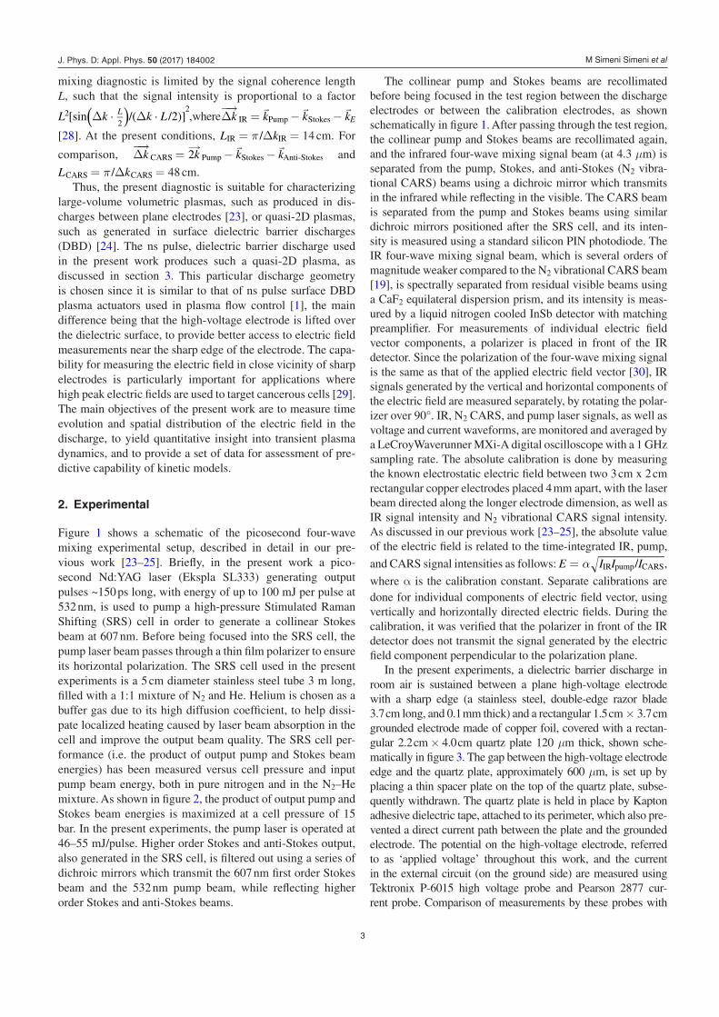
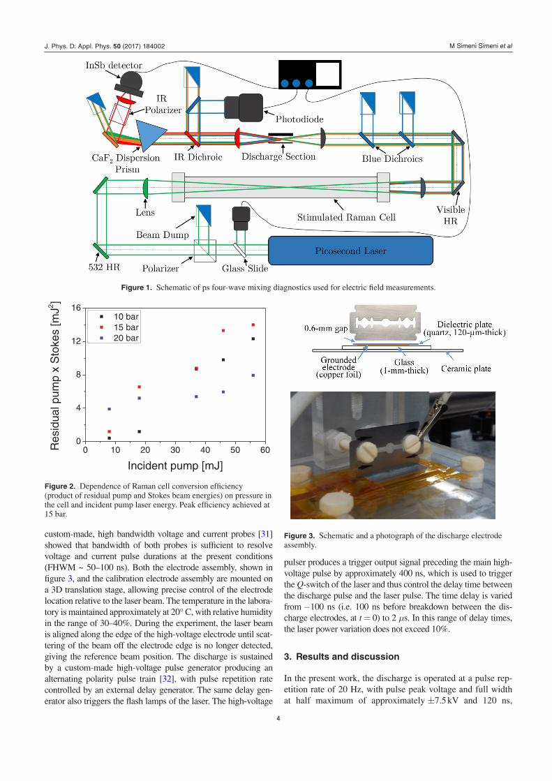
Figure 1 shows a schematic of the picosecond four-wave mixing experimental setup, described in detail in our pre-vious work [23–25]. Briefly, in the present work a pico-second Nd:YAG laser (Ekspla SL333) generating output pulses ~150 ps long, with energy of up to 100 mJ per pulse at 532 nm, is used to pump a high-pressure Stimulated Raman Shifting (SRS) cell in order to generate a collinear Stokes beam at 607 nm. Before being focused into the SRS cell, the pump laser beam passes through a thin film polarizer to ensure its horizontal polarization. The SRS cell used in the present experiments is a 5 cm diameter stainless steel tube 3 m long, filled with a 1:1 mixture of N2 and He. Helium is chosen as a buffer gas due to its high diffusion coefficient, to help dissi-pate localized heating caused by laser beam absorption in the cell and improve the output beam quality. The SRS cell per-formance (i.e. the product of output pump and Stokes beam energies) has been measured versus cell pressure and input pump beam energy, both in pure nitrogen and in the N2–He mixture. As shown in figure 2, the product of output pump and Stokes beam energies is maximized at a cell pressure of 15 bar. In the present experiments, the pump laser is operated at 46–55 mJ/pulse. Higher order Stokes and anti-Stokes output, also generated in the SRS cell, is filtered out using a series of dichroic mirrors which transmit the 607 nm first order Stokes beam and the 532 nm pump beam, while reflecting higher order Stokes and anti-Stokes beams.

The collinear pump and Stokes beams are recollimated before being focused in the test region between the discharge electrodes or between the calibration electrodes, as shown schematically in figure 1. After passing through the test region, the collinear pump and Stokes beams are recollimated again, and the infrared four-wave mixing signal beam (at 4.3 µm) is separated from the pump, Stokes, and anti-Stokes (N2 vibra-tional CARS) beams using a dichroic mirror which transmits in the infrared while reflecting in the visible. The CARS beam is separated from the pump and Stokes beams using similar dichroic mirrors positioned after the SRS cell, and its inten-sity is measured using a standard silicon PIN photodiode. The IR four-wave mixing signal beam, which is several orders of magnitude weaker compared to the N2 vibrational CARS beam [19], is spectrally separated from residual visible beams using a CaF2 equilateral dispersion prism, and its intensity is meas-ured by a liquid nitrogen cooled InSb detector with matching preamplifier. For measurements of individual electric field vector components, a polarizer is placed in front of the IR detector. Since the polarization of the four-wave mixing signal is the same as that of the applied electric field vector [30], IR signals generated by the vertical and horizontal components of the electric field are measured separately, by rotating the polar-izer over 90°. IR, N2 CARS, and pump laser signals, as well as voltage and current waveforms, are monitored and averaged by a LeCroyWaverunner MXi-A digital oscilloscope with a 1 GHz sampling rate. The absolute calibration is done by measuring the known electrostatic electric field between two 3 cm x 2 cm rectangular copper electrodes placed 4 mm apart, with the laser beam directed along the longer electrode dimension, as well as IR signal intensity and N2 vibrational CARS signal intensity. As discussed in our previous work [23–25], the absolute value of the electric field is related to the time-integrated IR, pump,

and CARS signal intensities as follows: /α=E I I IIR pump CARS,

where α is the calibration constant. Separate calibrations are done for individual components of electric field vector, using vertically and horizontally directed electric fields. During the calibration, it was verified that the polarizer in front of the IR detector does not transmit the signal generated by the electric field comp onent perpendicular to the polarization plane.

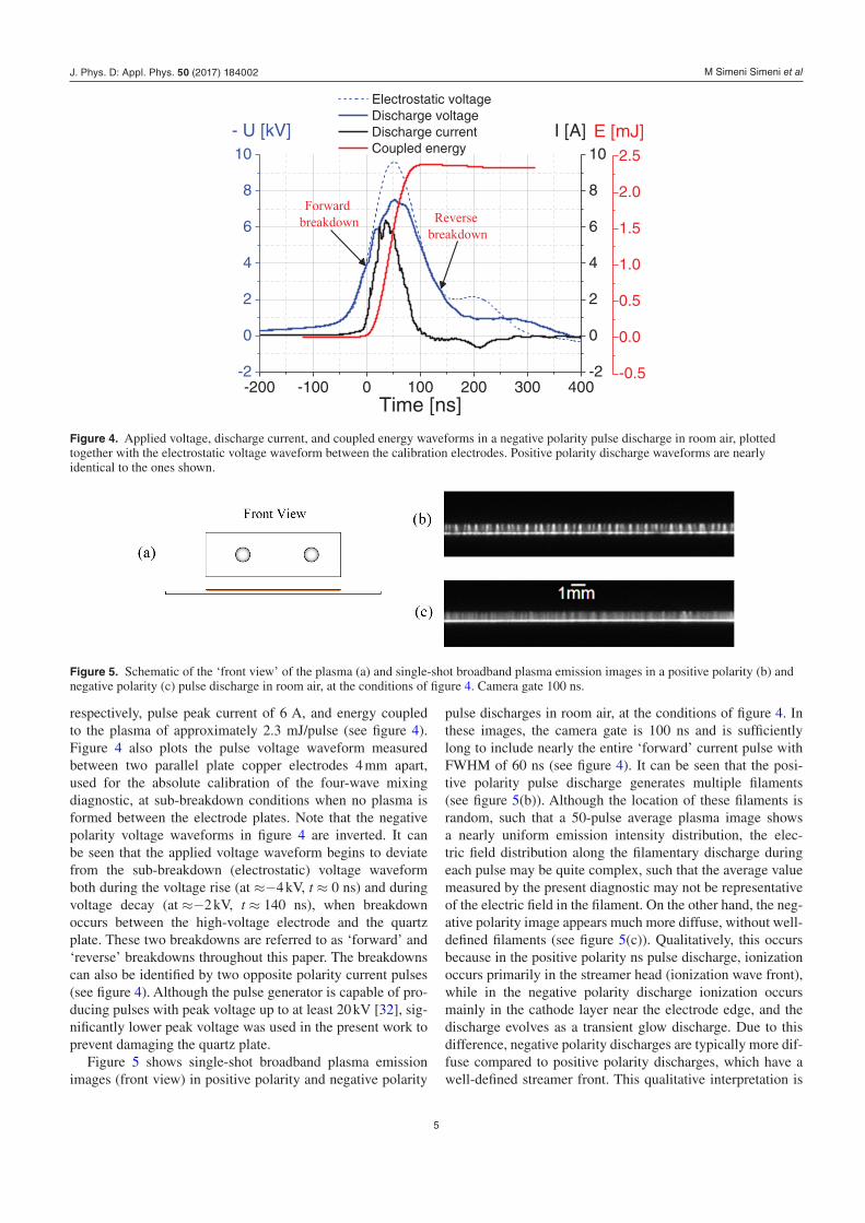
In the present experiments, a dielectric barrier discharge in room air is sustained between a plane high-voltage electrode with a sharp edge (a stainless steel, double-edge razor blade 3.7 cm long, and 0.1 mm thick) and a rectangular 1.5 cm × 3.7 cm grounded electrode made of copper foil, covered with a rectan-gular 2.2 cm × 4.0 cm quartz plate 120 µm thick, shown sche-matically in figure 3. The gap between the high-voltage electrode edge and the quartz plate, approximately 600 µm, is set up by placing a thin spacer plate on the top of the quartz plate, subse-quently withdrawn. The quartz plate is held in place by Kapton adhesive dielectric tape, attached to its perimeter, which also pre-vented a direct current path between the plate and the grounded electrode. The potential on the high-voltage electrode, referred to as ‘applied voltage’ throughout this work, and the current in the external circuit (on the ground side) are measured using Tektronix P-6015 high voltage probe and Pearson 2877 cur-rent probe. Comparison of measurements by these probes with

J. Phys. D: Appl. Phys. 50 (2017) 184002

M Simeni Simeni et al

4

custom-made, high bandwidth voltage and current probes [31] showed that bandwidth of both probes is sufficient to resolve voltage and current pulse durations at the present conditions (FHWM ~ 50–100 ns). Both the electrode assembly, shown in figure 3, and the calibration electrode assembly are mounted on a 3D translation stage, allowing precise control of the electrode location relative to the laser beam. The temperature in the labora-tory is maintained approximately at 20° C, with relative humidity in the range of 30–40%. During the experiment, the laser beam is aligned along the edge of the high-voltage electrode until scat-tering of the beam off the electrode edge is no longer detected, giving the reference beam position. The discharge is sustained by a custom-made high-voltage pulse generator producing an alternating polarity pulse train [32], with pulse repetition rate controlled by an external delay generator. The same delay gen-erator also triggers the flash lamps of the laser. The high-voltage

pulser produces a trigger output signal preceding the main high-voltage pulse by approximately 400 ns, which is used to trigger the Q-switch of the laser and thus control the delay time between the discharge pulse and the laser pulse. The time delay is varied from −100 ns (i.e. 100 ns before breakdown between the dis-charge electrodes, at t = 0) to 2 µs. In this range of delay times, the laser power variation does not exceed 10%.

3. Results and discussion

In the present work, the discharge is operated at a pulse rep-etition rate of 20 Hz, with pulse peak voltage and full width at half maximum of approximately ±7.5 kV and 120 ns,

Figure 1. Schematic of ps four-wave mixing diagnostics used for electric field measurements.

0 10 20 30 40 50 600

4

8

12

16Jm[

sekotS

xp

muplaudiseR

2 ]

Incident pump [mJ]

10 bar15 bar20 bar

Figure 2. Dependence of Raman cell conversion efficiency (product of residual pump and Stokes beam energies) on pressure in the cell and incident pump laser energy. Peak efficiency achieved at 15 bar.

Figure 3. Schematic and a photograph of the discharge electrode assembly.

J. Phys. D: Appl. Phys. 50 (2017) 184002

M Simeni Simeni et al

5

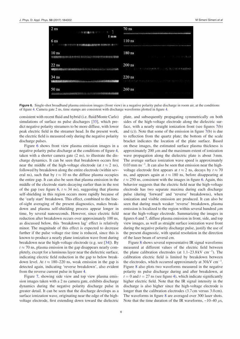
respectively, pulse peak current of 6 A, and energy coupled to the plasma of approximately 2.3 mJ/pulse (see figure 4). Figure  4 also plots the pulse voltage waveform measured between two parallel plate copper electrodes 4 mm apart, used for the absolute calibration of the four-wave mixing diagnostic, at sub-breakdown conditions when no plasma is formed between the electrode plates. Note that the negative polarity voltage waveforms in figure  4 are inverted. It can be seen that the applied voltage waveform begins to deviate from the sub-breakdown (electrostatic) voltage waveform both during the voltage rise (at ≈−4 kV, t ≈ 0 ns) and during voltage decay (at ≈−2 kV, t ≈ 140 ns), when breakdown occurs between the high-voltage electrode and the quartz plate. These two breakdowns are referred to as ‘forward’ and ‘reverse’ breakdowns throughout this paper. The breakdowns can also be identified by two opposite polarity current pulses (see figure 4). Although the pulse generator is capable of pro-ducing pulses with peak voltage up to at least 20 kV [32], sig-nificantly lower peak voltage was used in the present work to prevent damaging the quartz plate.

Figure 5 shows single-shot broadband plasma emission images (front view) in positive polarity and negative polarity

pulse discharges in room air, at the conditions of figure 4. In these images, the camera gate is 100 ns and is sufficiently long to include nearly the entire ‘forward’ current pulse with FWHM of 60 ns (see figure 4). It can be seen that the posi-tive polarity pulse discharge generates multiple filaments (see figure 5(b)). Although the location of these filaments is random, such that a 50-pulse average plasma image shows a nearly uniform emission intensity distribution, the elec-tric field distribution along the filamentary discharge during each pulse may be quite complex, such that the average value measured by the present diagnostic may not be representative of the electric field in the filament. On the other hand, the neg-ative polarity image appears much more diffuse, without well-defined filaments (see figure 5(c)). Qualitatively, this occurs because in the positive polarity ns pulse discharge, ionization occurs primarily in the streamer head (ionization wave front), while in the negative polarity discharge ionization occurs mainly in the cathode layer near the electrode edge, and the discharge evolves as a transient glow discharge. Due to this difference, negative polarity discharges are typically more dif-fuse compared to positive polarity discharges, which have a well-defined streamer front. This qualitative interpretation is

-200 -100 0 100 200 300 400-2

0

2

4

6

8

10

- U [kV]

Electrostatic voltage Discharge voltage Discharge current Coupled energy

Time [ns]

-2

0

2

4

6

8

10

I [A]

-0.5

0.0

0.5

1.0

1.5

2.0

2.5

Reverse breakdown

Forward breakdown

E [mJ]

Figure 4. Applied voltage, discharge current, and coupled energy waveforms in a negative polarity pulse discharge in room air, plotted together with the electrostatic voltage waveform between the calibration electrodes. Positive polarity discharge waveforms are nearly identical to the ones shown.

Figure 5. Schematic of the ‘front view’ of the plasma (a) and single-shot broadband plasma emission images in a positive polarity (b) and negative polarity (c) pulse discharge in room air, at the conditions of figure 4. Camera gate 100 ns.

J. Phys. D: Appl. Phys. 50 (2017) 184002

M Simeni Simeni et al

6

consistent with recent fluid and hybrid (i.e. fluid/Monte Carlo) simulations of surface ns pulse discharges [33], which pre-dict negative polarity streamers to be more diffuse, with lower peak electric field in the streamer head. In the present work, the electric field is measured only during the negative polarity discharge pulses.

Figure 6 shows front view plasma emission images in a negative polarity pulse discharge at the conditions of figure 4, taken with a shorter camera gate (2 ns), to illustrate the dis-charge dynamics. It can be seen that breakdown occurs first near the middle of the high-voltage electrode (at t ≈ 2 ns), followed by breakdown along the entire electrode (within sev-eral ns), such that by t ≈ 10 ns the diffuse plasma occupies the entire gap. It can also be seen that plasma emission in the middle of the electrode starts decaying earlier than in the rest of the gap (see figure  6, t ≈ 34 ns), suggesting that plasma self-shielding in this region occurs more rapidly because of the ‘early start’ breakdown. This effect, combined to the line-of-sight averaging of the present diagnostics, makes break-down and plasma self-shielding process appear longer in time, by several nanoseconds. However, since electric field reduction after breakdown occurs over approximately 100 ns, as discussed below, this ‘breakdown lag’ effect is relatively minor. The magnitude of this effect is expected to decrease further if the pulse voltage rise time is reduced, since this is known to produce a nearly plane ionization wave front during breakdown near the high-voltage electrode (e.g. see [34]). By t ≈ 70 ns, plasma emission in the gap disappears nearly com-pletely, except for a luminous layer near the dielectric surface, indicating electric field reduction in the gap to below break-down level. At t ≈ 180–220 ns, weak emission in the gap is detected again, indicating ‘reverse breakdown’, also evident from the reverse current pulse in figure 4.

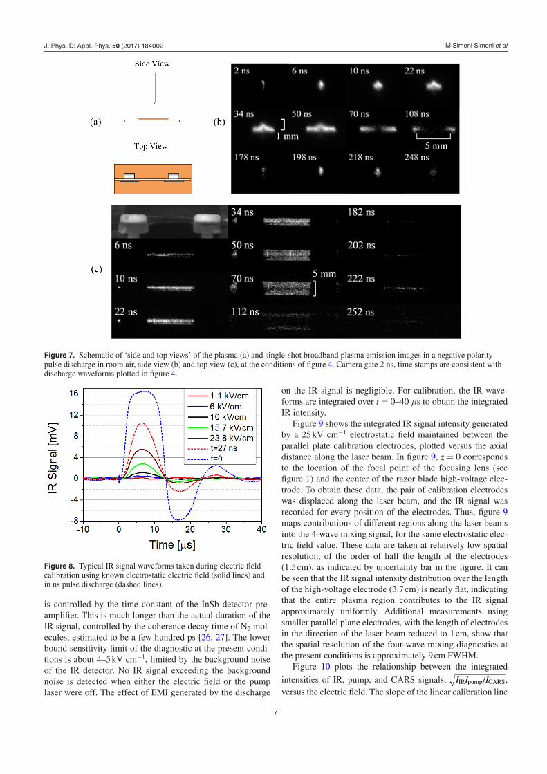
Figure 7, showing side view and top view plasma emis-sion images taken with a 2 ns camera gate, exhibits discharge dynamics during the negative polarity discharge pulse in greater detail. It can be seen that the discharge develops as a surface ionization wave, originating near the edge of the high-voltage electrode, first extending down toward the dielectric

plate, and subsequently propagating symmetrically on both sides of the high-voltage electrode along the dielectric sur-face, with a nearly straight ionization front (see figures 7(b) and (c)). Note that some of the emission in figure 7(b) is due to reflection from the quartz plate; the bottom of the scale bracket indicates the location of the plate surface. Based on these images, the estimated surface plasma thickness is approximately 200 µm and the maximum extent of ionization wave propagation along the dielectric plate is about 3 mm. The average surface ionization wave speed is approximately 0.03 mm ns−1. It can also be seen that emission near the high-voltage electrode first appears at t ≈ 2 ns, decays by t ≈ 70 ns, and appears again at t ≈ 180 ns, before disappearing at t ≈ 250 ns, consistent with the images in figure 6. Again, this behavior suggests that the electric field near the high-voltage electrode has two separate maxima during each discharge pulse (during ‘forward’ and ‘reverse’ breakdowns), when ionization and visible emission are produced. It can also be seen that during much weaker ‘reverse’ breakdown, plasma emission is localized to the region within several hundred µm near the high-voltage electrode. Summarizing the images in figures 6 and 7, diffuse plasma emission in front, side, and top view images, as well as straight surface ionization wave front during the negative polarity discharge pulse, justify the use of the present diagnostic, with spatial resolution in the direction of the laser beam of several cm.

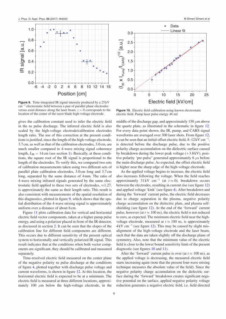
Figure 8 shows several representative IR signal waveforms measured at different values of the electric field between the plane calibration electrodes (at 1.1–23.8 kV cm−1). The calibration electric field is limited by breakdown between the electrodes, which occurred approximately at 30 kV cm−1. Figure 8 also plots two waveforms measured in the negative polarity ns pulse discharge during and after breakdown, at t = 0 and t = 27 ns (see figure 4), which indicate significantly higher electric field. Note that the IR signal intensity in the discharge is also higher since the high-voltage electrode is longer than the calibration electrodes (3.7 cm versus 3.0 cm). The waveforms in figure 8 are averaged over 300 laser shots. Note that the time duration of the IR waveforms, ~10–40 µs,

Figure 6. Single-shot broadband plasma emission images (front view) in a negative polarity pulse discharge in room air, at the conditions of figure 4. Camera gate 2 ns, time stamps are consistent with discharge waveforms plotted in figure 4.

J. Phys. D: Appl. Phys. 50 (2017) 184002

M Simeni Simeni et al

7

is controlled by the time constant of the InSb detector pre-amplifier. This is much longer than the actual duration of the IR signal, controlled by the coherence decay time of N2 mol-ecules, estimated to be a few hundred ps [26, 27]. The lower bound sensitivity limit of the diagnostic at the present condi-tions is about 4–5 kV cm−1, limited by the background noise of the IR detector. No IR signal exceeding the background noise is detected when either the electric field or the pump laser were off. The effect of EMI generated by the discharge

on the IR signal is negligible. For calibration, the IR wave-forms are integrated over t = 0–40 µs to obtain the integrated IR intensity.

Figure 9 shows the integrated IR signal intensity generated by a 25 kV cm−1 electrostatic field maintained between the parallel plate calibration electrodes, plotted versus the axial distance along the laser beam. In figure 9, z = 0 corresponds to the location of the focal point of the focusing lens (see figure 1) and the center of the razor blade high-voltage elec-trode. To obtain these data, the pair of calibration electrodes was displaced along the laser beam, and the IR signal was recorded for every position of the electrodes. Thus, figure 9 maps contributions of different regions along the laser beams into the 4-wave mixing signal, for the same electrostatic elec-tric field value. These data are taken at relatively low spatial resolution, of the order of half the length of the electrodes (1.5 cm), as indicated by uncertainty bar in the figure. It can be seen that the IR signal intensity distribution over the length of the high-voltage electrode (3.7 cm) is nearly flat, indicating that the entire plasma region contributes to the IR signal approximately uniformly. Additional measurements using smaller parallel plane electrodes, with the length of electrodes in the direction of the laser beam reduced to 1 cm, show that the spatial resolution of the four-wave mixing diagnostics at the present conditions is approximately 9 cm FWHM.

Figure 10 plots the relationship between the integrated

intensities of IR, pump, and CARS signals, /I I IIR pump CARS, versus the electric field. The slope of the linear calibration line

Figure 7. Schematic of ‘side and top views’ of the plasma (a) and single-shot broadband plasma emission images in a negative polarity pulse discharge in room air, side view (b) and top view (c), at the conditions of figure 4. Camera gate 2 ns, time stamps are consistent with discharge waveforms plotted in figure 4.

Figure 8. Typical IR signal waveforms taken during electric field calibration using known electrostatic electric field (solid lines) and in ns pulse discharge (dashed lines).

J. Phys. D: Appl. Phys. 50 (2017) 184002

M Simeni Simeni et al

8

gives the calibration constant used to infer the electric field in the ns pulse discharge. The inferred electric field is also scaled by the high-voltage electrode/calibration electrodes length ratio. The use of this correction at the present condi-tions is justified, since the length of the high-voltage electrode, 3.7 cm, as well as that of the calibration electrodes, 3.0 cm, are much smaller compared to 4-wave mixing signal coherence length, LIR = 14 cm (see section 1). Basically, at these condi-tions, the square root of the IR signal is proportional to the length of the electrodes. To verify this, we compared two sets of calibration measurements taken using two different sets of parallel plate calibration electrodes, 3.0 cm long and 3.7 cm long, separated by the same distance of 4 mm. The ratio of 4-wave mixing infrared signals generated by the same elec-trostatic field applied to these two sets of electrodes, ≈1.27, is approximately the same as their length ratio. This result is also consistent with measurements of the spatial resolution of this diagnostics, plotted in figure 9, which shows that the spa-tial distribution of the 4-wave mixing signal is approximately uniform over a distance of about 6 cm.

Figure 11 plots calibration data for vertical and horizontal electric field vector components, taken at a higher pump pulse energy, and using a polarizer placed in front of the IR detector, as discussed in section 2. It can be seen that the slopes of the calibration line for different field components are different. This occurs due to different sensitivity of the present optical system to horizontally and vertically polarized IR signal. This result indicates that at the conditions when both vector comp-onents are significant, they should be calibrated and measured separately.

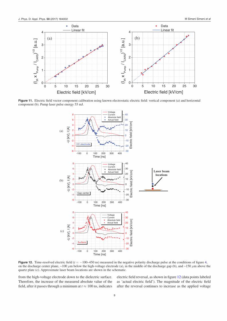
Time-resolved electric field measured on the center plane of the negative polarity ns pulse discharge at the conditions of figure 4, plotted together with discharge pulse voltage and current waveforms, is shown in figure 12. At this location, the horizontal electric field is expected to be at a minimum. The electric field is measured at three different locations, approxi-mately 100 µm below the high-voltage electrode, in the

middle of the discharge gap, and approximately 150 µm above the quartz plate, as illustrated in the schematic in figure 12. For every data point shown, the IR, pump, and CARS signal waveforms are averaged over 300 laser shots. From figure 12, it can be seen that an initial offset electric field, 8–12 kV cm−1, is detected before the discharge pulse, due to the positive polarity charge accumulation on the dielectric surface caused by breakdown during the lower peak voltage (+3.8 kV), posi-tive polarity ‘pre-pulse’ generated approximately 6 µs before the main discharge pulse. As expected, the offset electric field is higher near the sharp edge of the high-voltage electrode.

As the applied voltage begins to increase, the electric field also increases following the voltage. When the field reaches approximately 31 kV cm−1 (at t ≈ 0), breakdown occurs between the electrodes, resulting in current rise (see figure 12) and applied voltage ‘kink’ (see figure 4). After breakdown and during the ‘forward’ current pulse, the electric field decreases due to charge separation in the plasma, negative polarity charge accumulation on the dielectric plate, and plasma self-shielding (see figure 12). At the end of the ‘forward’ current pulse, however (at t ≈ 100 ns), the electric field is not reduced to zero, as expected. The minimum electric field near the high-voltage electrode, measured at t ≈ 100 ns, is approximately 4 kV cm−1 (see figure 12). This may be caused by slight mis-alignment of the high-voltage electrode and the laser beam, such that the data are taken slightly off the discharge plane of symmetry. Also, note that the minimum value of the electric field is close to the lower bound sensitivity limit of the present diagnostic (see figures 10 and 11).

After the ‘forward’ current pulse is over (at t ≈ 100 ns), as the applied voltage is decreasing, the measured electric field starts increasing again (note that the present four-wave mixing technique measures the absolute value of the field). Since the negative polarity charge accumulation on the dielectric sur-face during the ‘forward’ breakdown creates significant nega-tive potential on the surface, applied negative polarity voltage reduction generates a negative electric field, i.e. field directed

-6 -4 -2 0 2 4 6 8 10 12 14 160.0

0.2

0.4

0.6

0.8

1.0

].u.a[langisRI

Position [cm]

Figure 9. Time-integrated IR signal intensity produced by a 25 kV cm−1 electrostatic field between a pair of parallel plane electrodes versus axial distance along the laser beam. z = 0 corresponds to the location of the center of the razor blade high-voltage electrode.

0 5 10 15 20 25

0.0

0.5

1.0

1.5

2.0

2.5

3.0

Data Linear fit

(IIR

Ix

pmu

P/I

SR

AC

)2/1

].u.a[

Electric field [kV/cm]

Figure 10. Electric field calibration using known electrostatic electric field. Pump laser pulse energy 46 mJ.

J. Phys. D: Appl. Phys. 50 (2017) 184002

M Simeni Simeni et al

9

from the high-voltage electrode down to the dielectric surface. Therefore, the increase of the measured absolute value of the field, after it passes through a minimum at t ≈ 100 ns, indicates

electric field reversal, as shown in figure 12 (data points labeled as ‘actual electric field’). The magnitude of the electric field after the reversal continues to increase as the applied voltage

(b)

0 5 10 15 20 25 300

1

2

3

4

Data Linear fit

(IIR

Ix

pmu

P /

IS

RA

C)1/

2].u.a[

Electric field [kV/cm]

(a)

0 5 10 15 20 25 300

1

2

3

4

Data Linear fit

(IIR

Ix

pmu

P /

IS

RA

C)1/

2].u.a[

Electric field [kV/cm]

Figure 11. Electric field vector component calibration using known electrostatic electric field: vertical component (a) and horizontal component (b). Pump laser pulse energy 55 mJ.

(a)

(b)

(c)

Laser beamlocations

-100 0 100 200 300 400-6

-4

-2

0

2

4

6

8 Voltage Current Absolute field Actual field

Time [ns]

]A[I,]

Vk[U-

-30

-20

-10

0

10

20

30

40

Ele

ctric

fiel

d [k

V/c

m]

HV electrode

-100 0 100 200 300 400-6

-4

-2

0

2

4

6

8 Voltage Current Absolute field Actual field

Time [ns]

]A[I,]

Vk[U-

-30

-20

-10

0

10

20

30

40

Ele

ctric

fiel

d [k

V/c

m]

Gap center

-100 0 100 200 300 400-6

-4

-2

0

2

4

6

8 Voltage Current Absolute field Actual field

Time [ns]

]A[I,]

Vk[U-

-30

-20

-10

0

10

20

30

40

Ele

ctric

fiel

d [k

V/c

m]

Surface

Figure 12. Time-resolved electric field (t = −100–450 ns) measured in the negative polarity discharge pulse at the conditions of figure 4, on the discharge center plane, ~100 µm below the high-voltage electrode (a), in the middle of the discharge gap (b), and ~150 µm above the quartz plate (c). Approximate laser beam locations are shown in the schematic.

J. Phys. D: Appl. Phys. 50 (2017) 184002

M Simeni Simeni et al

10

is reduced, until breakdown occurs again, at t ≈ 180 ns. The ‘reverse’ breakdown results in the ‘reverse’, opposite polarity current pulse with peak current of about 0.7 A (see figure 12), as well as plasma emission near the high-voltage electrode, shown in figures 6 and 7. During the ‘reverse’ breakdown, at t ≈ 200–250 ns, the magnitude of the field decreases again, due to charge separation in the plasma, until the ‘reverse’ current pulse is over. After this, the magnitude of the field continues to increase as the applied voltage is gradually reduced to zero at t ≈ 300–450 ns (see figure 12).

Summarizing the data shown in figure  12, the present measurements indicate that the electric field near the high-voltage electrode (approximately 100 µm away) peaks when it reaches breakdown threshold, which is close to DC break-down value for a relatively long voltage pulse used in the pre-sent work. Peak electric field further away from the electrode remains about the same, close to breakdown threshold. This was verified by moving the laser beam vertically along the discharge center plane, at the forward breakdown moment and monitoring the 4-wave mixing IR signal intensity.

Time-resolved electric field evolution at these condi-tions, on a longer time scale, (t = −100 ns–2 µs), are shown in figure  13. It can be seen that the electric field gradually decreases, most likely due to surface charge neutralization by transport of opposite polarity charges from the plasma [23]. However, the residual electric field remains quite significant even 2 µs after the discharge pulse, 8–15 kV cm−1, due to surface charge accumulation on the dielectric surface. This is consistent with the electric field offset near the high-voltage electrode before the discharge pulse, 8–12 kV (see figure 12), caused by the positive polarity ‘pre-pulse’, although, as expected, the offset/residual electric field reverses polarity along with the applied voltage pulse polarity. Measurements at longer delay times after the discharge pulse become signifi-cantly less accurate, due to the reduction of pump laser power when the Q-switch delay time is increased.

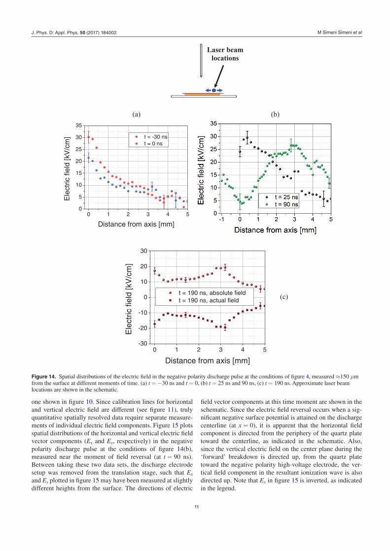
Figure 14 plots spatial distributions of the electric field, measured approximately 150 µm from the surface in the nega-tive polarity discharge at the conditions of figure 4, at different

moments of time during the discharge pulse. Figure  14(a) plots the electric field before breakdown, at t = −30 ns, and at the moment when forward breakdown begins, at t = 0 ns. In both cases, electric field distributions are essentially elec-trostatic, with well pronounced maxima on the center plane of the electrode assembly. The electric field decreases with the distance from the center plane, indicating that the effect of surface charge accumulation from the lower amplitude pre-pulse, resulting in the offset field at t < 0 (see figure 12(a)), is significant only near the high-voltage electrode.

Figure 14(b) plots the electric field soon after ‘forward’ breakdown, at t = 25 ns, and at the moment near electric field reversal near the high-voltage electrode, t = 90 ns (see figure  12). The data set near the field reversal is taken at a higher spatial resolution, 100 µm. It can be seen clearly that after breakdown the electric field maximum is moving away from the high voltage electrode, as a surface ionization wave, consistent with plasma emission images in figure  7. From figure 14(b), it is apparent that the electric field distribution near the field reversal is nearly symmetric about the center plane, as expected, although the field measured on the center plane is not reduced to zero. As discussed before, this is likely due to slight misalignment of the laser beam, which may be not exactly parallel to the high-voltage electrode. The electric field near field reversal reaches maximum at x = 2.8–3.1 mm, consistent with plasma emission images taken at t = 70 ns, 108 ns, and 112 ns, which indicate the extent of surface ioniz-ation wave propagation of x ≈ 2.5–3.0 mm (see figures 7(b) and (c)). The electric field distribution does not exhibit a sharp drop typical for a well-defined ionization wave front, detected in our previous measurements in a surface ionization wave in hydrogen at 200 Torr [24]. The field decreases both ahead and behind the broad maximum, approaching the detection limit near the plane of symmetry (see figure 14(b)).

Figure 14(c) plots the electric field distribution at t = 190 ns, when the field near the high-voltage electrode reaches a local maximum after the field reversal, right before the ‘reverse’ breakdown occurs (see figure  12). Figure  14(c) plots both the measured absolute value of the electric field and the ‘actual’ electric field, shown to be negative since at this moment both the vertical and the horizontal field comp-onents appear to be negative (i.e. directed down and toward the center plane, respectively), as discussed below. At this time moment, the applied voltage is low, approximately –1 kV (see figure 12), such that the field is controlled primarily by the negative polarity surface charge accumulated on the quartz plate during propagation of the surface ionization wave fol-lowing the forward breakdown. Again, the absolute value of the field peaks at the axial distance of x ≈ 3 mm, consistent with the maximum extent of ionization wave propagation determined from plasma emission images (see figures 6 and 7). This peak, with field reduction at x > 3 mm, is likely due to the ‘edge effect’ of the surface charge layer deposited on the quartz plate by the surface ionization wave, near its maximum extent.

Spatial distributions of the electric field plotted in figure 14 are inferred from the data using the calibration line obtained without the polarizer in front of the IR detector, such as the

0 500 1000 1500 2000-6

-4

-2

0

2

4

6

8

Voltage Current HV electrode Gap center Surface

Time [ns]

]A[I,]

Vk[U-

-30

-20

-10

0

10

20

30

40

Ele

ctric

fiel

d [k

V/c

m]

Figure 13. Time-resolved electric field (t = −100 ns–2 µs) measured in the negative polarity discharge pulse at the conditions of figure 4, on the discharge center plane. Approximate laser beam locations are shown in the schematic in figure 12.

J. Phys. D: Appl. Phys. 50 (2017) 184002

M Simeni Simeni et al

11

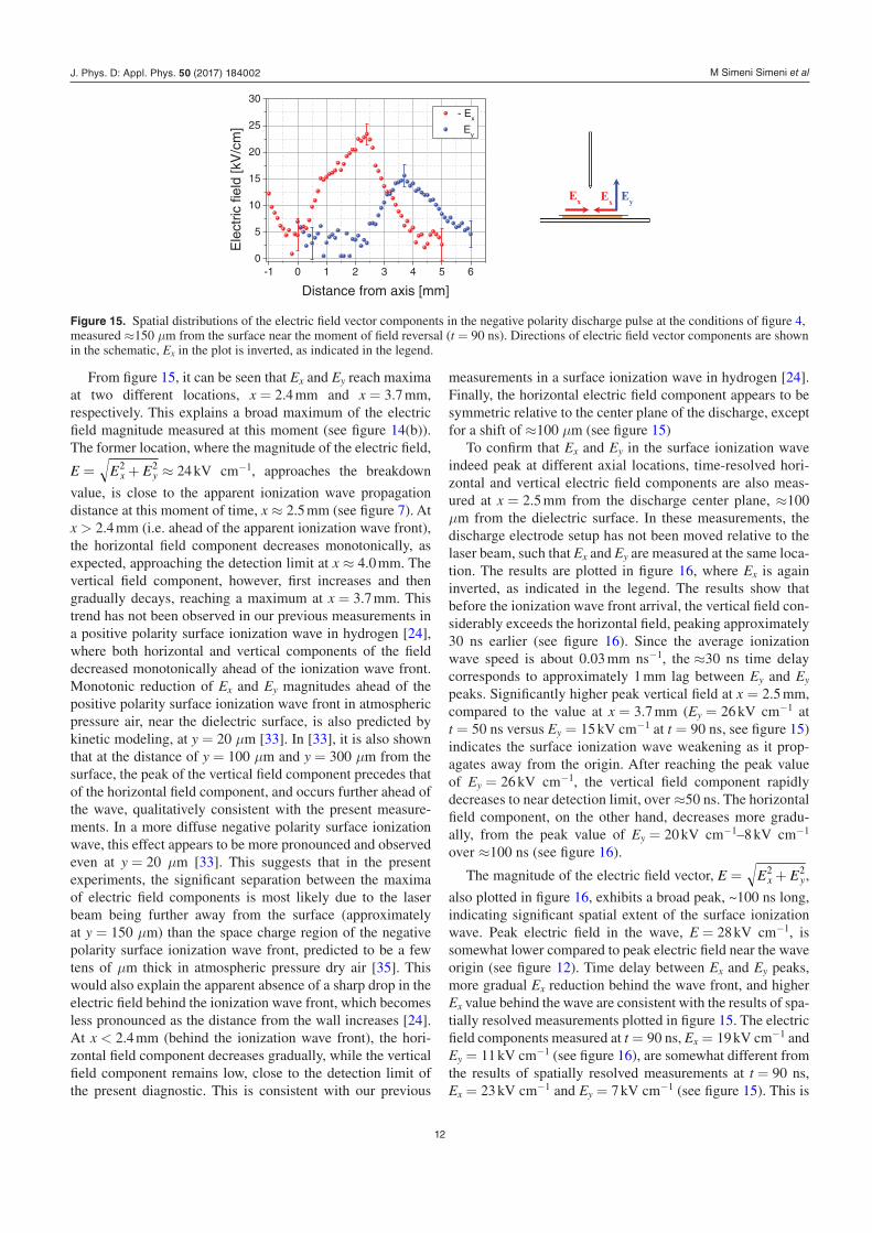
one shown in figure 10. Since calibration lines for horizontal and vertical electric field are different (see figure  11), truly quantitative spatially resolved data require separate measure-ments of individual electric field components. Figure 15 plots spatial distributions of the horizontal and vertical electric field vector components (Ex and Ey, respectively) in the negative polarity discharge pulse at the conditions of figure  14(b), measured near the moment of field reversal (at t = 90 ns). Between taking these two data sets, the discharge electrode setup was removed from the translation stage, such that Ex and Ey plotted in figure 15 may have been measured at slightly different heights from the surface. The directions of electric

field vector components at this time moment are shown in the schematic. Since the electric field reversal occurs when a sig-nificant negative surface potential is attained on the discharge centerline (at x = 0), it is apparent that the horizontal field component is directed from the periphery of the quartz plate toward the centerline, as indicated in the schematic. Also, since the vertical electric field on the center plane during the ‘forward’ breakdown is directed up, from the quartz plate toward the negative polarity high-voltage electrode, the ver-tical field component in the resultant ionization wave is also directed up. Note that Ex in figure 15 is inverted, as indicated in the legend.

Laser beam locations

0 1 2 3 4 50

5

10

15

20

25

30

35

t = -30 ns t = 0 ns

]mc/

Vk[dleif

cirtcelE

Distance from axis [mm]

0 1 2 3 4 5-30

-20

-10

0

10

20

30

t = 190 ns, absolute field t = 190 ns, actual field

]mc/

Vk[dleif

cirtcelE

Distance from axis [mm]

(c)

(a) (b)

Figure 14. Spatial distributions of the electric field in the negative polarity discharge pulse at the conditions of figure 4, measured ≈150 µm from the surface at different moments of time. (a) t = −30 ns and t = 0, (b) t = 25 ns and 90 ns, (c) t = 190 ns. Approximate laser beam locations are shown in the schematic.

J. Phys. D: Appl. Phys. 50 (2017) 184002

M Simeni Simeni et al

12

From figure 15, it can be seen that Ex and Ey reach maxima at two different locations, x = 2.4 mm and x = 3.7 mm, respectively. This explains a broad maximum of the electric field magnitude measured at this moment (see figure 14(b)). The former location, where the magnitude of the electric field,

= +E E Ex y2 2 ≈ 24 kV cm−1, approaches the breakdown

value, is close to the apparent ionization wave propagation distance at this moment of time, x ≈ 2.5 mm (see figure 7). At x > 2.4 mm (i.e. ahead of the apparent ionization wave front), the horizontal field component decreases monotonically, as expected, approaching the detection limit at x ≈ 4.0 mm. The vertical field component, however, first increases and then gradually decays, reaching a maximum at x = 3.7 mm. This trend has not been observed in our previous measurements in a positive polarity surface ionization wave in hydrogen [24], where both horizontal and vertical components of the field decreased monotonically ahead of the ionization wave front. Monotonic reduction of Ex and Ey magnitudes ahead of the positive polarity surface ionization wave front in atmospheric pressure air, near the dielectric surface, is also predicted by kinetic modeling, at y = 20 µm [33]. In [33], it is also shown that at the distance of y = 100 µm and y = 300 µm from the surface, the peak of the vertical field component precedes that of the horizontal field component, and occurs further ahead of the wave, qualitatively consistent with the present measure-ments. In a more diffuse negative polarity surface ionization wave, this effect appears to be more pronounced and observed even at y = 20 µm [33]. This suggests that in the present experiments, the significant separation between the maxima of electric field components is most likely due to the laser beam being further away from the surface (approximately at y = 150 µm) than the space charge region of the negative polarity surface ionization wave front, predicted to be a few tens of µm thick in atmospheric pressure dry air [35]. This would also explain the apparent absence of a sharp drop in the electric field behind the ionization wave front, which becomes less pronounced as the distance from the wall increases [24]. At x < 2.4 mm (behind the ionization wave front), the hori-zontal field component decreases gradually, while the vertical field component remains low, close to the detection limit of the present diagnostic. This is consistent with our previous

measurements in a surface ionization wave in hydrogen [24]. Finally, the horizontal electric field comp onent appears to be symmetric relative to the center plane of the discharge, except for a shift of ≈100 µm (see figure 15)

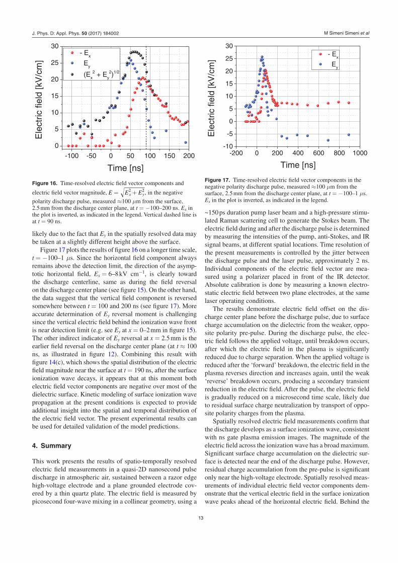
To confirm that Ex and Ey in the surface ionization wave indeed peak at different axial locations, time-resolved hori-zontal and vertical electric field components are also meas-ured at x = 2.5 mm from the discharge center plane, ≈100 µm from the dielectric surface. In these measurements, the discharge electrode setup has not been moved relative to the laser beam, such that Ex and Ey are measured at the same loca-tion. The results are plotted in figure 16, where Ex is again inverted, as indicated in the legend. The results show that before the ionization wave front arrival, the vertical field con-siderably exceeds the horizontal field, peaking approximately 30 ns earlier (see figure  16). Since the average ioniz ation wave speed is about 0.03 mm ns−1, the ≈30 ns time delay corresponds to approximately 1 mm lag between Ey and Ey peaks. Significantly higher peak vertical field at x = 2.5 mm, compared to the value at x = 3.7 mm (Ey = 26 kV cm−1 at t = 50 ns versus Ey = 15 kV cm−1 at t = 90 ns, see figure 15) indicates the surface ionization wave weakening as it prop-agates away from the origin. After reaching the peak value of Ey = 26 kV  cm−1, the vertical field component rapidly decreases to near detection limit, over ≈50 ns. The horizontal field component, on the other hand, decreases more gradu-ally, from the peak value of Ey = 20 kV cm−1–8 kV cm−1 over ≈100 ns (see figure 16).

The magnitude of the electric field vector, = +E E Ex y2 2,

also plotted in figure 16, exhibits a broad peak, ~100 ns long, indicating significant spatial extent of the surface ionization wave. Peak electric field in the wave, E = 28 kV cm−1, is somewhat lower compared to peak electric field near the wave origin (see figure 12). Time delay between Ex and Ey peaks, more gradual Ex reduction behind the wave front, and higher Ex value behind the wave are consistent with the results of spa-tially resolved measurements plotted in figure 15. The electric field components measured at t = 90 ns, Ex = 19 kV cm−1 and Ey = 11 kV cm−1 (see figure 16), are somewhat different from the results of spatially resolved measurements at t = 90 ns, Ex = 23 kV cm−1 and Ey = 7 kV cm−1 (see figure 15). This is

EyE

xE

x

-1 0 1 2 3 4 5 60

5

10

15

20

25

30- E

x

Ey

]mc/

Vk[dleif

cirtcelE

Distance from axis [mm]

Figure 15. Spatial distributions of the electric field vector components in the negative polarity discharge pulse at the conditions of figure 4, measured ≈150 µm from the surface near the moment of field reversal (t = 90 ns). Directions of electric field vector components are shown in the schematic, Ex in the plot is inverted, as indicated in the legend.

J. Phys. D: Appl. Phys. 50 (2017) 184002

M Simeni Simeni et al

13

likely due to the fact that Ey in the spatially resolved data may be taken at a slightly different height above the surface.

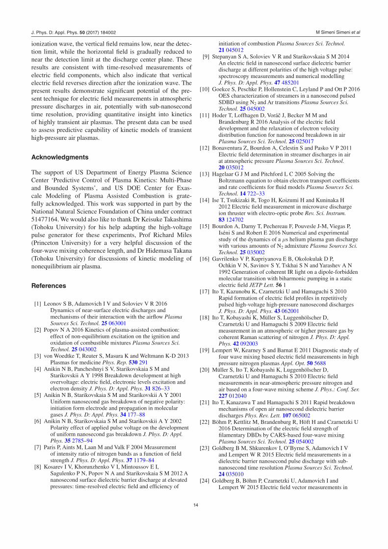
Figure 17 plots the results of figure 16 on a longer time scale, t = −100–1 µs. Since the horizontal field component always remains above the detection limit, the direction of the asymp-totic horizontal field, Ex = 6–8 kV cm−1, is clearly toward the discharge centerline, same as during the field reversal on the discharge center plane (see figure 15). On the other hand, the data suggest that the vertical field component is reversed somewhere between t = 100 and 200 ns (see figure 17). More accurate determination of Ey reversal moment is challenging since the vertical electric field behind the ionization wave front is near detection limit (e.g. see Ey at x = 0–2 mm in figure 15). The other indirect indicator of Ey reversal at x = 2.5 mm is the earlier field reversal on the discharge center plane (at t ≈ 100 ns, as illustrated in figure  12). Combining this result with figure 14(c), which shows the spatial distribution of the electric field magnitude near the surface at t = 190 ns, after the surface ionization wave decays, it appears that at this moment both electric field vector components are negative over most of the dielectric surface. Kinetic modeling of surface ionization wave propagation at the present conditions is expected to provide additional insight into the spatial and temporal distribution of the electric field vector. The present experimental results can be used for detailed validation of the model predictions.

4. Summary

This work presents the results of spatio-temporally resolved electric field measurements in a quasi-2D nanosecond pulse discharge in atmospheric air, sustained between a razor edge high-voltage electrode and a plane grounded electrode cov-ered by a thin quartz plate. The electric field is measured by picosecond four-wave mixing in a collinear geometry, using a

~150 ps duration pump laser beam and a high-pressure stimu-lated Raman scattering cell to generate the Stokes beam. The electric field during and after the discharge pulse is determined by measuring the intensities of the pump, anti-Stokes, and IR signal beams, at different spatial locations. Time resolution of the present measurements is controlled by the jitter between the discharge pulse and the laser pulse, approximately 2 ns. Individual components of the electric field vector are mea-sured using a polarizer placed in front of the IR detector. Absolute calibration is done by measuring a known electro-static electric field between two plane electrodes, at the same laser operating conditions.

The results demonstrate electric field offset on the dis-charge center plane before the discharge pulse, due to surface charge accumulation on the dielectric from the weaker, oppo-site polarity pre-pulse. During the discharge pulse, the elec-tric field follows the applied voltage, until breakdown occurs, after which the electric field in the plasma is significantly reduced due to charge separation. When the applied voltage is reduced after the ‘forward’ breakdown, the electric field in the plasma reverses direction and increases again, until the weak ‘reverse’ breakdown occurs, producing a secondary transient reduction in the electric field. After the pulse, the electric field is gradually reduced on a microsecond time scale, likely due to residual surface charge neutralization by transport of oppo-site polarity charges from the plasma.

Spatially resolved electric field measurements confirm that the discharge develops as a surface ionization wave, consistent with ns gate plasma emission images. The magnitude of the electric field across the ionization wave has a broad maximum. Significant surface charge accumulation on the dielectric sur-face is detected near the end of the discharge pulse. However, residual charge accumulation from the pre-pulse is significant only near the high-voltage electrode. Spatially resolved meas-urements of individual electric field vector components dem-onstrate that the vertical electric field in the surface ionization wave peaks ahead of the horizontal electric field. Behind the

-100 -50 0 50 100 150 200

0

5

10

15

20

25

30- E

x

Ey

(Ex2 + E

y2)1/2

]mc/

Vk[dleif

cirtcelE

Time [ns]

Figure 16. Time-resolved electric field vector components and

electric field vector magnitude, = +E E Ex y2 2, in the negative

polarity discharge pulse, measured ≈100 µm from the surface, 2.5 mm from the discharge center plane, at t = −100–200 ns. Ex in the plot is inverted, as indicated in the legend. Vertical dashed line is at t = 90 ns.

-200 0 200 400 600 800 1000-10

-5

0

5

10

15

20

25

30- E

x

Ey

]mc/

Vk[dleif

cirtcelE

Time [ns]

Figure 17. Time-resolved electric field vector components in the negative polarity discharge pulse, measured ≈100 µm from the surface, 2.5 mm from the discharge center plane, at t = −100–1 µs. Ex in the plot is inverted, as indicated in the legend.

J. Phys. D: Appl. Phys. 50 (2017) 184002

M Simeni Simeni et al

14

ionization wave, the vertical field remains low, near the detec-tion limit, while the horizontal field is gradually reduced to near the detection limit at the discharge center plane. These results are consistent with time-resolved measurements of electric field components, which also indicate that vertical electric field reverses direction after the ionization wave. The present results demonstrate significant potential of the pre-sent technique for electric field measurements in atmospheric pressure discharges in air, potentially with sub-nanosecond time resolution, providing quantitative insight into kinetics of highly transient air plasmas. The present data can be used to assess predictive capability of kinetic models of transient high-pressure air plasmas.

Acknowledgments

The support of US Department of Energy Plasma Science Center ‘Predictive Control of Plasma Kinetics: Multi-Phase and Bounded Systems’, and US DOE Center for Exas-cale Modeling of Plasma Assisted Combustion is grate-fully acknowledged. This work was supported in part by the National Natural Science Foundation of China under contract 51477164. We would also like to thank Dr Keisuke Takashima (Tohoku University) for his help adapting the high-voltage pulse generator for these experiments, Prof Richard Miles (Princeton University) for a very helpful discussion of the four-wave mixing coherence length, and Dr Hidemasa Takana (Tohoku University) for discussions of kinetic modeling of nonequilibrium air plasma.

References

[1] Leonov S B, Adamovich I V and Soloviev V R 2016 Dynamics of near-surface electric discharges and mechanisms of their interaction with the airflow Plasma Sources Sci. Technol. 25 063001

[2] Popov N A 2016 Kinetics of plasma-assisted combustion: effect of non-equilibrium excitation on the ignition and oxidation of combustible mixtures Plasma Sources Sci. Technol. 25 043002

[3] von Woedtke T, Reuter S, Masura K and Weltmann K-D 2013 Plasmas for medicine Phys. Rep. 530 291

[4] Anikin N B, Pancheshnyi S V, Starikovskaia S M and Starikovskii A Y 1998 Breakdown development at high overvoltage: electric field, electronic levels excitation and electron density J. Phys. D: Appl. Phys. 31 826–33

[5] Anikin N B, Starikovskaia S M and Starikovskii A Y 2001 Uniform nanosecond gas breakdown of negative polarity: initiation form electrode and propagation in molecular gases J. Phys. D: Appl. Phys. 34 177–88

[6] Anikin N B, Starikovskaia S M and Starikovskii A Y 2002 Polarity effect of applied pulse voltage on the development of uniform nanosecond gas breakdown J. Phys. D: Appl. Phys. 35 2785–94

[7] Paris P, Aints M, Laan M and Valk F 2004 Measurement of intensity ratio of nitrogen bands as a function of field strength J. Phys. D: Appl. Phys. 37 1179–84

[8] Kosarev I V, Khorunzhenko V I, Mintoussov E I, Sagulenko P N, Popov N A and Starikovskaia S M 2012 A nanosecond surface dielectric barrier discharge at elevated pressures: time-resolved electric field and efficiency of

initiation of combustion Plasma Sources Sci. Technol. 21 045012

[9] Stepanyan S A, Soloviev V R and Starikovskaia S M 2014 An electric field in nanosecond surface dielectric barrier discharge at different polarities of the high voltage pulse: spectroscopy measurements and numerical modelling J. Phys. D: Appl. Phys. 47 485201

[10] Goekce S, Peschke P, Hollenstein C, Leyland P and Ott P 2016 OES characterization of streamers in a nanosecond pulsed SDBD using N2 and Ar transitions Plasma Sources Sci. Technol. 25 045002

[11] Hoder T, Loffhagen D, Voráč J, Becker M M and Brandenburg R 2016 Analysis of the electric field development and the relaxation of electron velocity distribution function for nanosecond breakdown in air Plasma Sources Sci. Technol. 25 025017

[12] Bonaventura Z, Bourdon A, Celestin S and Pasko V P 2011 Electric field determination in streamer discharges in air at atmospheric pressure Plasma Sources Sci. Technol. 20 035012

[13] Hagelaar G J M and Pitchford L C 2005 Solving the Boltzmann equation to obtain electron transport coefficients and rate coefficients for fluid models Plasma Sources Sci. Technol. 14 722–33

[14] Ise T, Tsukizaki R, Togo H, Koizumi H and Kuninaka H 2012 Electric field measurement in microwave discharge ion thruster with electro-optic probe Rev. Sci. Instrum. 83 124702

[15] Bourdon A, Darny T, Pechereau F, Pouvesle J-M, Viegas P, Iséni S and Robert E 2016 Numerical and experimental study of the dynamics of a µs helium plasma gun discharge with various amounts of N2 admixture Plasma Sources Sci. Technol. 25 035002

[16] Gavrilenko V P, Kupriyanova E B, Okolokulak D P, Ochkin V N, Savinov S Y, Tskhai S N and Yarashev A N 1992 Generation of coherent IR light on a dipole-forbidden molecular transition with biharmonic pumping in a static electric field JETP Lett. 56 1

[17] Ito T, Kazunobu K, Czarnetzki U and Hamaguchi S 2010 Rapid formation of electric field profiles in repetitively pulsed high-voltage high-pressure nanosecond discharges J. Phys. D: Appl. Phys. 43 062001

[18] Ito T, Kobayashi K, Müller S, Luggenhölscher D, Czarnetzki U and Hamaguchi S 2009 Electric field measurement in an atmospheric or higher pressure gas by coherent Raman scattering of nitrogen J. Phys. D: Appl. Phys. 42 092003

[19] Lempert W, Kearney S and Barnat E 2011 Diagnostic study of four wave mixing based electric field measurements in high pressure nitrogen plasmas Appl. Opt. 50 5688

[20] Müller S, Ito T, Kobayashi K, Luggenhölscher D, Czarnetzki U and Hamaguchi S 2010 Electric field measurements in near-atmospheric pressure nitrogen and air based on a four-wave mixing scheme J. Phys.: Conf. Ser. 227 012040

[21] Ito T, Kanazawa T and Hamaguchi S 2011 Rapid breakdown mechanisms of open air nanosecond dielectric barrier discharges Phys. Rev. Lett. 107 065002

[22] Böhm P, Kettlitz M, Brandenburg R, Höft H and Czarnetzki U 2016 Determination of the electric field strength of filamentary DBDs by CARS-based four-wave mixing Plasma Sources Sci. Technol. 25 054002

[23] Goldberg B M, Shkurenkov I, O’Byrne S, Adamovich I V and Lempert W R 2015 Electric field measurements in a dielectric barrier nanosecond pulse discharge with sub-nanosecond time resolution Plasma Sources Sci. Technol. 24 035010

[24] Goldberg B, Böhm P, Czarnetzki U, Adamovich I and Lempert W 2015 Electric field vector measurements in

J. Phys. D: Appl. Phys. 50 (2017) 184002

M Simeni Simeni et al

15

a surface ionization wave discharge Plasma Sources Sci. Technol. 24 055017

[25] Goldberg B, Shkurenkov I, Adamovich I V and Lempert W R 2016 Electric field vector measurements in an AC dielectric barrier discharge overlapped with a nanosecond pulse discharge Plasma Sources Sci. Technol. 25 045008

[26] Kulatilaka W D, Hsu P S, Stauffer H U, Gord J R and Roy S 2010 Direct measurement of rotationally resolved H2 Q-branch Raman coherence lifetimes using time-resolved picosecond coherent anti-Stokes Raman scattering Appl. Phys. Lett. 97 081112

[27] Knopp G, Beaud P, Radi P, Tulej M, Bougie B, Cannavo D and Gerber T 2002 Pressure-dependent N2 Q-branch fs-CARS measurements J. Raman Spectrosc. 33 861

[28] Lempert W R and Adamovich I V 2014 Coherent anti-Stokes Raman scattering and spontaneous Raman scattering diagnostics of nonequilibrium plasmas and flows J. Phys. D: Appl. Phys. 47 433001

[29] Nuccitelli R, Pliquett U, Chen X, Ford W, Swanson R J, Beebe S J, Kolb J F and Schoenbach K H 2006 Nanosecond pulsed electric fields cause melanomas to self-destruct Biochem. Biophys. Res. Commun. 343 351

[30] Tskhai S N, Akimov D A, Mitko S V, Ochkin V N, Serdyuchenko A Y, Sidorov-Biryukov D A, Sinyaev D V and Zheltikov A M 2001 Time-resolved

polarization-sensitive measurements of the electric field in a sliding discharge by means of dc field-induced coherent Raman scattering J. Raman Spectrosc. 32 177–81

[31] Takashima K, Yin Z and Adamovich I V 2013 Measurements and kinetic modeling of energy coupling in volume and surface nanosecond pulse discharges Plasma Sources Sci. Technol. 22 015013

[32] Takashima K, Adamovich I V, Xiong Z, Kushner M J, Starikovskaia S, Czarnetzki U and Luggenhölscher D 2011 Experimental and modeling analysis of fast ionization wave discharge propagation in a rectangular geometry Phys. Plasmas 18 083505

[33] Babaeva N Y, Tereshonok D V and Naidis G V 2016 Fluid and hybrid modeling of nanosecond surface discharges: effect of polarity and secondary electrons emission Plasma Sources Sci. Technol. 25 044008

[34] Starikovskii A, Nikipelov A, Nudnova M and Roupassov D 2009 SDBD plasma actuator with nanosecond pulse-periodic discharge Plasma Sources Sci. Technol. 18 034015

[35] Soloviev V R, Krivtsov V M, Shcherbanev S A and Starikovskaia S M 2017 Evolution of nanosecond surface dielectric barrier discharge for negative polarity of a voltage pulse Plasma Sources Sci. Technol. 26 014001

J. Phys. D: Appl. Phys. 50 (2017) 184002