Eigenvalues, eigenvectors, andeigenspaces of linear operators

Math 130 Linear AlgebraD Joyce, Fall 2015

Eigenvalues and eigenvectors. We’re lookingat linear operators on a vector space V , that is,linear transformations x 7→ T (x) from the vectorspace V to itself.

When V has finite dimension n with a specifiedbasis β, then T is described by a square n×n matrixA = [T ]β.

We’re particularly interested in the study the ge-ometry of these transformations in a way that wecan’t when the transformation goes from one vec-tor space to a different vector space, namely, we’llcompare the original vector x to its image T (x).

Some of these vectors will be sent to other vectorson the same line, that is, a vector x will be sent toa scalar multiple λx of itself.

Definition 1. For a given linear operator T : V →V , a nonzero vector x and a constant scalar λ arecalled an eigenvector and its eigenvalue, respec-tively, when T (x) = λx. For a given eigenvalueλ, the set of all x such that T (x) = λx is calledthe λ-eigenspace. The set of all eigenvalues for atransformation is called its spectrum.

When the operator T is described by a matrixA, then we’ll associate the eigenvectors, eigenval-ues, eigenspaces, and spectrum to A as well. AsA directly describes a linear operator on F n, we’lltake its eigenspaces to be subsets of F n.

Theorem 2. Each λ-eigenspace is a subspace of V .

Proof. Suppose that x and y are λ-eigenvectors andc is a scalar. Then

T (x+cy) = T (x)+cT (y) = λx+cλy = λ(x+cy).

Therefore x + cy is also a λ-eigenvector. Thus,the set of λ-eigenvectors form a subspace of F n.

q.e.d.

One reason these eigenvalues and eigenspaces areimportant is that you can determine many of theproperties of the transformation from them, andthat those properties are the most important prop-erties of the transformation.

These are matrix invariants. Note that theeigenvalues, eigenvectors, and eigenspaces of a lin-ear transformation were defined in terms of thetransformation, not in terms of a matrix that de-scribes the transformation relative to a particu-lar basis. That means that they are invariants ofsquare matrices under change of basis. Recall thatif A and B represent the transformation with re-spect to two different bases, then A and B are con-jugate matrices, that is, B = P−1AP where P isthe transition matrix between the two bases. Theeigenvalues are numbers, and they’ll be the samefor A and B. The corresponding eigenspaces willbe isomorphic as subspaces of F n under the linearoperator of conjugation by P . Thus we have thefollowing theorem.

Theorem 3. The eigenvalues of a square matrix Aare the same as any conjugate matrix B = P−1APof A. Furthermore, each λ-eigenspace for A is iso-morphic to the λ-eigenspace for B. In particular,the dimensions of each λ-eigenspace are the samefor A and B.

When 0 is an eigenvalue. It’s a special situa-tion when a transformation has 0 an an eigenvalue.That means Ax = 0 for some nontrivial vector x.In general, a 0-eigenspaces is the solution space ofthe homogeneous equation Ax = 0, what we’vebeen calling the null space of A, and its dimensionwe’ve been calling the nullity of A. Since a squarematrix is invertible if and only if it’s nullity is 0, wecan conclude the following theorem.

Theorem 4. A square matrix is invertible if andonly if 0 is not one of its eigenvalues. Put another

1

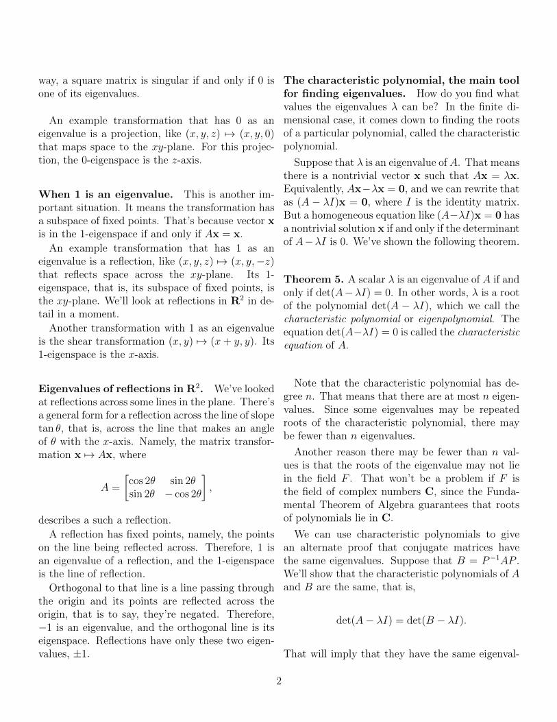
way, a square matrix is singular if and only if 0 isone of its eigenvalues.

An example transformation that has 0 as aneigenvalue is a projection, like (x, y, z) 7→ (x, y, 0)that maps space to the xy-plane. For this projec-tion, the 0-eigenspace is the z-axis.

When 1 is an eigenvalue. This is another im-portant situation. It means the transformation hasa subspace of fixed points. That’s because vector xis in the 1-eigenspace if and only if Ax = x.

An example transformation that has 1 as aneigenvalue is a reflection, like (x, y, z) 7→ (x, y,−z)that reflects space across the xy-plane. Its 1-eigenspace, that is, its subspace of fixed points, isthe xy-plane. We’ll look at reflections in R2 in de-tail in a moment.

Another transformation with 1 as an eigenvalueis the shear transformation (x, y) 7→ (x + y, y). Its1-eigenspace is the x-axis.

Eigenvalues of reflections in R2. We’ve lookedat reflections across some lines in the plane. There’sa general form for a reflection across the line of slopetan θ, that is, across the line that makes an angleof θ with the x-axis. Namely, the matrix transfor-mation x 7→ Ax, where

A =

[cos 2θ sin 2θsin 2θ − cos 2θ

],

describes a such a reflection.

A reflection has fixed points, namely, the pointson the line being reflected across. Therefore, 1 isan eigenvalue of a reflection, and the 1-eigenspaceis the line of reflection.

Orthogonal to that line is a line passing throughthe origin and its points are reflected across theorigin, that is to say, they’re negated. Therefore,−1 is an eigenvalue, and the orthogonal line is itseigenspace. Reflections have only these two eigen-values, ±1.

The characteristic polynomial, the main toolfor finding eigenvalues. How do you find whatvalues the eigenvalues λ can be? In the finite di-mensional case, it comes down to finding the rootsof a particular polynomial, called the characteristicpolynomial.

Suppose that λ is an eigenvalue of A. That meansthere is a nontrivial vector x such that Ax = λx.Equivalently, Ax−λx = 0, and we can rewrite thatas (A − λI)x = 0, where I is the identity matrix.But a homogeneous equation like (A−λI)x = 0 hasa nontrivial solution x if and only if the determinantof A−λI is 0. We’ve shown the following theorem.

Theorem 5. A scalar λ is an eigenvalue of A if andonly if det(A−λI) = 0. In other words, λ is a rootof the polynomial det(A − λI), which we call thecharacteristic polynomial or eigenpolynomial. Theequation det(A−λI) = 0 is called the characteristicequation of A.

Note that the characteristic polynomial has de-gree n. That means that there are at most n eigen-values. Since some eigenvalues may be repeatedroots of the characteristic polynomial, there maybe fewer than n eigenvalues.

Another reason there may be fewer than n val-ues is that the roots of the eigenvalue may not liein the field F . That won’t be a problem if F isthe field of complex numbers C, since the Funda-mental Theorem of Algebra guarantees that rootsof polynomials lie in C.

We can use characteristic polynomials to givean alternate proof that conjugate matrices havethe same eigenvalues. Suppose that B = P−1AP .We’ll show that the characteristic polynomials of Aand B are the same, that is,

det(A− λI) = det(B − λI).

That will imply that they have the same eigenval-

2

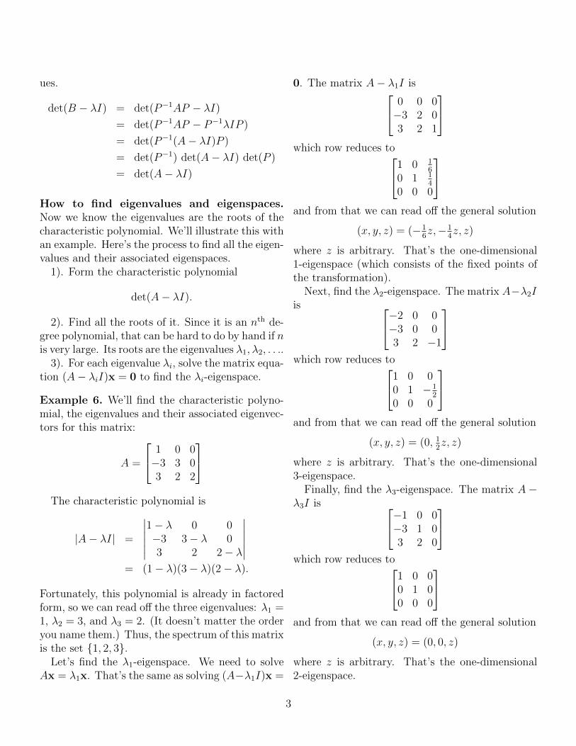
ues.

det(B − λI) = det(P−1AP − λI)

= det(P−1AP − P−1λIP )

= det(P−1(A− λI)P )

= det(P−1) det(A− λI) det(P )

= det(A− λI)

How to find eigenvalues and eigenspaces.Now we know the eigenvalues are the roots of thecharacteristic polynomial. We’ll illustrate this withan example. Here’s the process to find all the eigen-values and their associated eigenspaces.

1). Form the characteristic polynomial

det(A− λI).

2). Find all the roots of it. Since it is an nth de-gree polynomial, that can be hard to do by hand if nis very large. Its roots are the eigenvalues λ1, λ2, . . ..

3). For each eigenvalue λi, solve the matrix equa-tion (A− λiI)x = 0 to find the λi-eigenspace.

Example 6. We’ll find the characteristic polyno-mial, the eigenvalues and their associated eigenvec-tors for this matrix:

A =

1 0 0−3 3 03 2 2

The characteristic polynomial is

|A− λI| =

∣∣∣∣∣∣1− λ 0 0−3 3− λ 03 2 2− λ

∣∣∣∣∣∣= (1− λ)(3− λ)(2− λ).

Fortunately, this polynomial is already in factoredform, so we can read off the three eigenvalues: λ1 =1, λ2 = 3, and λ3 = 2. (It doesn’t matter the orderyou name them.) Thus, the spectrum of this matrixis the set {1, 2, 3}.

Let’s find the λ1-eigenspace. We need to solveAx = λ1x. That’s the same as solving (A−λ1I)x =

0. The matrix A− λ1I is 0 0 0−3 2 03 2 1

which row reduces to1 0 1

6

0 1 14

0 0 0

and from that we can read off the general solution

(x, y, z) = (−16z,−1

4z, z)

where z is arbitrary. That’s the one-dimensional1-eigenspace (which consists of the fixed points ofthe transformation).

Next, find the λ2-eigenspace. The matrix A−λ2Iis −2 0 0

−3 0 03 2 −1

which row reduces to1 0 0

0 1 −12

0 0 0

and from that we can read off the general solution

(x, y, z) = (0, 12z, z)

where z is arbitrary. That’s the one-dimensional3-eigenspace.

Finally, find the λ3-eigenspace. The matrix A−λ3I is −1 0 0

−3 1 03 2 0

which row reduces to1 0 0

0 1 00 0 0

and from that we can read off the general solution

(x, y, z) = (0, 0, z)

where z is arbitrary. That’s the one-dimensional2-eigenspace.

3

Math 130 Home Page athttp://math.clarku.edu/~ma130/

4