1

Econ 7331 Professor Chris Murray Econometrics 1 McElhinney 211 D Spring 2015 cjmurray@uh.edu

Midterm Exam Write your answers on one side of the blank white paper that I have given you. Do not write your answers on this exam. You must explain your answers. If you are confused about a question or you think it is unclear, please ask for clarification before answering. When testing a hypothesis, make sure to write down the null and alternative, the critical value(s), the test statistic, and your decision (reject or fail to reject). Use tests with 5% size. Unless otherwise specified, use 2-sided alternative hypotheses. 1. Statistical Properties of the OLS Estimator Consider the classical linear regression model uXy += β , with deterministic regressors and ),0(~ 2

nIu σ . a. Derive the mean and covariance matrix of .ˆ

OLSβ (5 points) b. Is OLSβ efficient? Be explicit. (5 points) Now assume that the error terms are Gaussian; ),0(~ 2

nINu σ . c. Does your answer to part b change? (2 points)

d. Consider the statistic, ( ) [ ] ( )2

11 ˆ')'('ˆ

σββ rRRXXRrR −−

−−

, which we know has a 2jχ

distribution in finite samples, but is not feasible since 2σ is unknown. Discuss how to deal with this nuisance parameter problem to get the feasible F-statistic. (10 points) e. Write down (i.e. do not derive) the F-statistic in terms of restricted and unrestricted sums of squared residuals and R-squares. (5 points)

2

2. Numerical Properties of the OLS Estimator Consider the OLS decomposition of y into its explained and unexplained components: uyy ˆˆ += . a. Write y and u in terms of projection matrices. (5 points) b. Interpret these projection matrices. (5 points) c. In what sense is the OLS decomposition an orthogonal decomposition? Be specific. (5 points) 3. Consider the partitioned regression model: uXXy ++= 2211 ββ . The Frisch-Waugh theorem tell us that we can write the OLS estimator for 1β as ( ) **

11*

1*11 ''ˆ yXXX −

=β or ( ) yMXXMX 21

11211 ''ˆ −=β

where ')'( 2

12222 XXXXIM −−= , yMy 2

* ≡ , and 12*1 XMX ≡

a. Interpret 2M , *y , and *

1X . (15 points) b. Interpret ρ in the Frisch-Waugh context when the regression model is ttt uybtay +++= −1ρ . (10 points). Hint: Think of 1X and 2X as

=

−1

1

0

1

Ty

yy

X

,

=

T

X

1

2111

2

.

3

4. Consider the following two regression models:

uXMXy ++= 22111 βα

vXMy += 221 β Demonstrate that these two regressions must yield the same estimates of 2β . (10 points) (This is problem #6 from ps2)

4

5. Consider the following regression model with Normal errors: iiiii uXXXY ++++= 3322110 ββββ where ),0(~ 2σiidNui . a. Test the following hypothesis: (10 points)

0:0:

01

00

≠=

ββ

HH

b. Test the following hypothesis using a confidence interval: (10 points)

82:82:

321

320

≠+=+

ββββ

HH

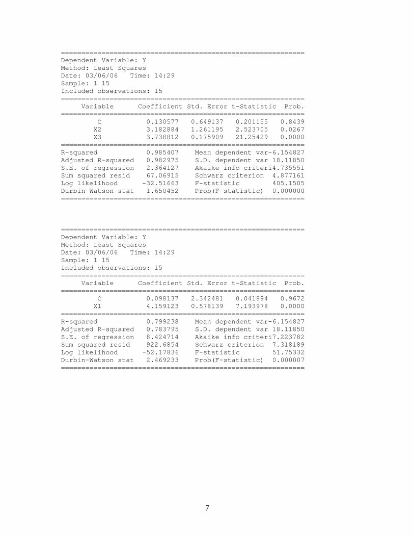
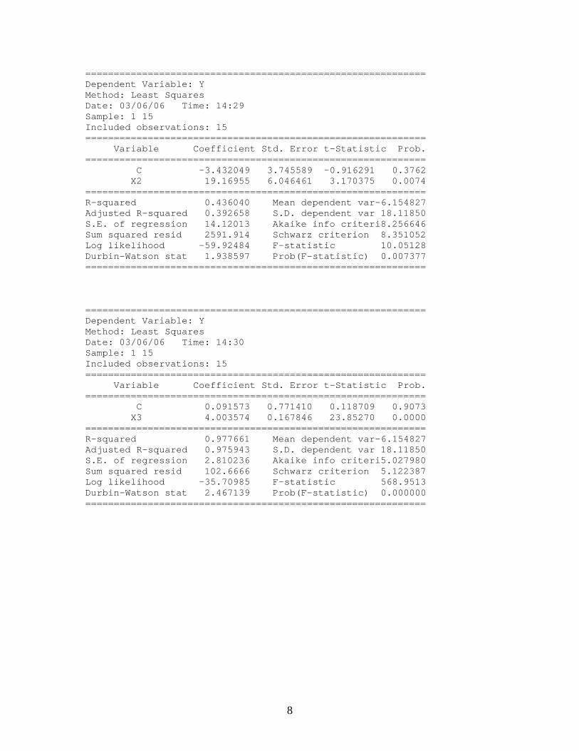
c. Test the following hypotheses: (10 points)

0 ,0,0:0 ,0,0:

3211

3210

≠≠≠===

ββββββ

HH

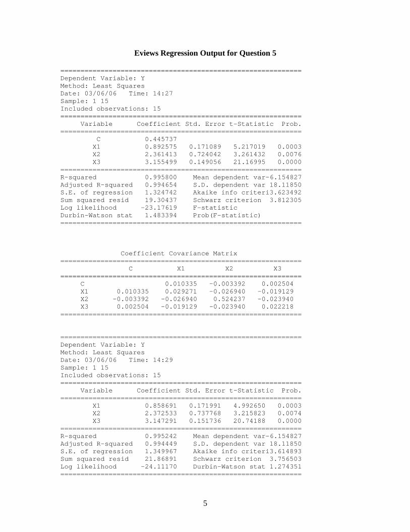
5

Eviews Regression Output for Question 5 ============================================================ Dependent Variable: Y Method: Least Squares Date: 03/06/06 Time: 14:27 Sample: 1 15 Included observations: 15 ============================================================ Variable Coefficient Std. Error t-Statistic Prob. ============================================================ C 0.445737 X1 0.892575 0.171089 5.217019 0.0003 X2 2.361413 0.724042 3.261432 0.0076 X3 3.155499 0.149056 21.16995 0.0000 ============================================================ R-squared 0.995800 Mean dependent var-6.154827 Adjusted R-squared 0.994654 S.D. dependent var 18.11850 S.E. of regression 1.324742 Akaike info criteri3.623492 Sum squared resid 19.30437 Schwarz criterion 3.812305 Log likelihood -23.17619 F-statistic Durbin-Watson stat 1.483394 Prob(F-statistic) ============================================================ Coefficient Covariance Matrix ============================================================ C X1 X2 X3 ============================================================ C 0.010335 -0.003392 0.002504 X1 0.010335 0.029271 -0.026940 -0.019129 X2 -0.003392 -0.026940 0.524237 -0.023940 X3 0.002504 -0.019129 -0.023940 0.022218 ============================================================ ============================================================ Dependent Variable: Y Method: Least Squares Date: 03/06/06 Time: 14:29 Sample: 1 15 Included observations: 15 ============================================================ Variable Coefficient Std. Error t-Statistic Prob. ============================================================ X1 0.858691 0.171991 4.992650 0.0003 X2 2.372533 0.737768 3.215823 0.0074 X3 3.147291 0.151736 20.74188 0.0000 ============================================================ R-squared 0.995242 Mean dependent var-6.154827 Adjusted R-squared 0.994449 S.D. dependent var 18.11850 S.E. of regression 1.349967 Akaike info criteri3.614893 Sum squared resid 21.86891 Schwarz criterion 3.756503 Log likelihood -24.11170 Durbin-Watson stat 1.274351 ============================================================

6

============================================================ Dependent Variable: Y Method: Least Squares Date: 03/06/06 Time: 14:29 Sample: 1 15 Included observations: 15 ============================================================ Variable Coefficient Std. Error t-Statistic Prob. ============================================================ C 0.090116 2.278498 0.039550 0.9691 X1 3.609472 0.699869 5.157357 0.0002 X2 5.761485 4.367186 1.319267 0.2117 ============================================================ R-squared 0.824668 Mean dependent var-6.154827 Adjusted R-squared 0.795446 S.D. dependent var 18.11850 S.E. of regression 8.194568 Akaike info criteri7.221677 Sum squared resid 805.8114 Schwarz criterion 7.363287 Log likelihood -51.16257 F-statistic 28.22080 Durbin-Watson stat 2.573820 Prob(F-statistic) 0.000029 ============================================================ ============================================================ Dependent Variable: Y Method: Least Squares Date: 03/06/06 Time: 14:29 Sample: 1 15 Included observations: 15 ============================================================ Variable Coefficient Std. Error t-Statistic Prob. ============================================================ C 0.461016 0.495082 0.931191 0.3701 X1 1.013924 0.224238 4.521646 0.0007 X3 3.263335 0.195164 16.72102 0.0000 ============================================================ R-squared 0.991738 Mean dependent var-6.154827 Adjusted R-squared 0.990361 S.D. dependent var 18.11850 S.E. of regression 1.778848 Akaike info criteri4.166665 Sum squared resid 37.97159 Schwarz criterion 4.308275 Log likelihood -28.24999 F-statistic 720.2144 Durbin-Watson stat 2.269623 Prob(F-statistic) 0.000000 ============================================================

7

============================================================ Dependent Variable: Y Method: Least Squares Date: 03/06/06 Time: 14:29 Sample: 1 15 Included observations: 15 ============================================================ Variable Coefficient Std. Error t-Statistic Prob. ============================================================ C 0.130577 0.649137 0.201155 0.8439 X2 3.182884 1.261195 2.523705 0.0267 X3 3.738812 0.175909 21.25429 0.0000 ============================================================ R-squared 0.985407 Mean dependent var-6.154827 Adjusted R-squared 0.982975 S.D. dependent var 18.11850 S.E. of regression 2.364127 Akaike info criteri4.735551 Sum squared resid 67.06915 Schwarz criterion 4.877161 Log likelihood -32.51663 F-statistic 405.1505 Durbin-Watson stat 1.650452 Prob(F-statistic) 0.000000 ============================================================ ============================================================ Dependent Variable: Y Method: Least Squares Date: 03/06/06 Time: 14:29 Sample: 1 15 Included observations: 15 ============================================================ Variable Coefficient Std. Error t-Statistic Prob. ============================================================ C 0.098137 2.342481 0.041894 0.9672 X1 4.159123 0.578139 7.193978 0.0000 ============================================================ R-squared 0.799238 Mean dependent var-6.154827 Adjusted R-squared 0.783795 S.D. dependent var 18.11850 S.E. of regression 8.424714 Akaike info criteri7.223782 Sum squared resid 922.6854 Schwarz criterion 7.318189 Log likelihood -52.17836 F-statistic 51.75332 Durbin-Watson stat 2.469233 Prob(F-statistic) 0.000007 ============================================================

8

============================================================ Dependent Variable: Y Method: Least Squares Date: 03/06/06 Time: 14:29 Sample: 1 15 Included observations: 15 ============================================================ Variable Coefficient Std. Error t-Statistic Prob. ============================================================ C -3.432049 3.745589 -0.916291 0.3762 X2 19.16955 6.046461 3.170375 0.0074 ============================================================ R-squared 0.436040 Mean dependent var-6.154827 Adjusted R-squared 0.392658 S.D. dependent var 18.11850 S.E. of regression 14.12013 Akaike info criteri8.256646 Sum squared resid 2591.914 Schwarz criterion 8.351052 Log likelihood -59.92484 F-statistic 10.05128 Durbin-Watson stat 1.938597 Prob(F-statistic) 0.007377 ============================================================ ============================================================ Dependent Variable: Y Method: Least Squares Date: 03/06/06 Time: 14:30 Sample: 1 15 Included observations: 15 ============================================================ Variable Coefficient Std. Error t-Statistic Prob. ============================================================ C 0.091573 0.771410 0.118709 0.9073 X3 4.003574 0.167846 23.85270 0.0000 ============================================================ R-squared 0.977661 Mean dependent var-6.154827 Adjusted R-squared 0.975943 S.D. dependent var 18.11850 S.E. of regression 2.810236 Akaike info criteri5.027980 Sum squared resid 102.6666 Schwarz criterion 5.122387 Log likelihood -35.70985 F-statistic 568.9513 Durbin-Watson stat 2.467139 Prob(F-statistic) 0.000000 ============================================================