Final Review

ECON 1123

Sebastian James

(Slides prepared by Bo Jackson and Hanley Chiang)

I. The Big Picture • For much of this course, our aim has been to estimate the

causal effect of X on Y - Causal effect: Effect that would be measured in an ideal

randomized controlled experiment • We choose an estimator β̂ , a function of the observations in

our sample, to estimate the true effect β • Every estimator has a sampling distribution

o Over repeated samples, the estimator produces a distribution of estimates

o This distribution of estimates has a mean, variance, etc.

• We want the sampling distribution of the estimator to have certain nice properties: o Unbiased: ββ =)ˆ(E . Over repeated samples (each of

size n), the mean of our estimates would be the true population value β .

o Consistent: β̂ converges in probability to β . As n increases, the distribution of β̂ becomes narrower and narrower around β .

o Small variance.

II. Multiple Linear Regression

To estimate the multiple regression model uXXY KK ++++= βββ ...110 , the Ordinary Least Squares (OLS) estimators K ..., βββ ˆ,ˆ,ˆ

10 minimize the sum of squared residuals (“prediction mistakes”). • Usually, there is one independent variable of interest ( 1X ).

The other regressors ( 2X , 3X ,…, KX ) are control variables. • Which controls should you include? Any variable whose

omission would cause omitted variable bias in 1̂β : o The variable affects Y; and o The variable is correlated with 1X .

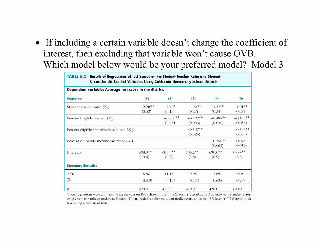
• If including a certain variable doesn’t change the coefficient of interest, then excluding that variable won’t cause OVB. Which model below would be your preferred model? Model 3

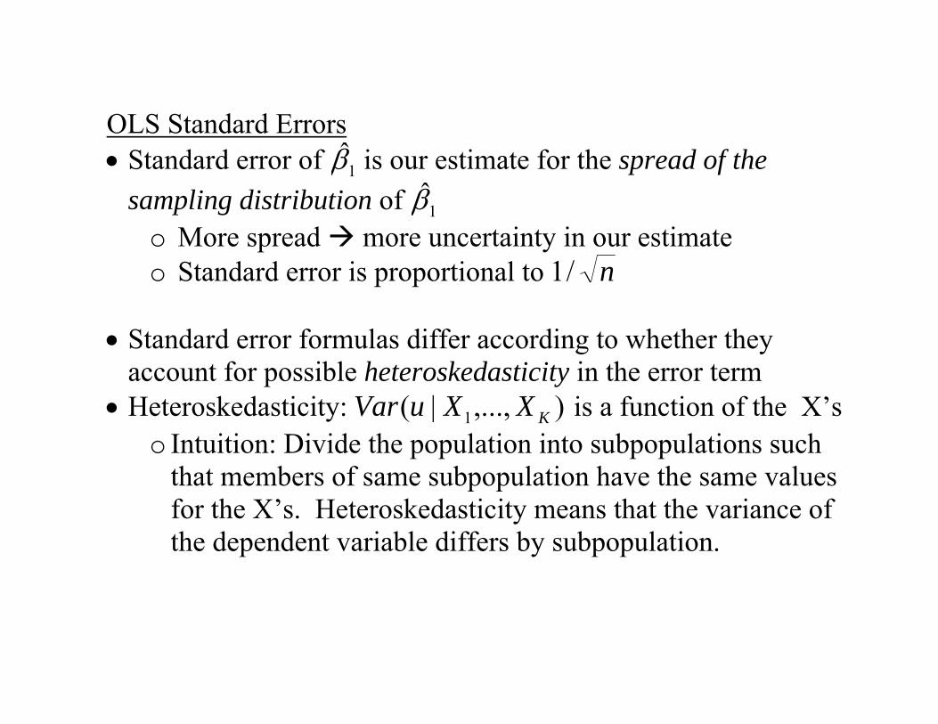
OLS Standard Errors • Standard error of 1̂β is our estimate for the spread of the

sampling distribution of 1̂β o More spread more uncertainty in our estimate o Standard error is proportional to n/1

• Standard error formulas differ according to whether they

account for possible heteroskedasticity in the error term • Heteroskedasticity: ),...,|( 1 KXXuVar is a function of the X’s

o Intuition: Divide the population into subpopulations such that members of same subpopulation have the same values for the X’s. Heteroskedasticity means that the variance of the dependent variable differs by subpopulation.

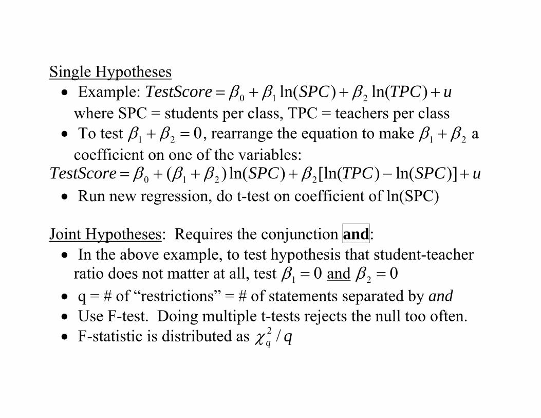
Single Hypotheses • Example: uTPCSPCTestScore +++= )ln()ln( 210 βββ

where SPC = students per class, TPC = teachers per class • To test 021 =+ ββ , rearrange the equation to make 21 ββ + a

coefficient on one of the variables: uSPCTPCSPCTestScore +−+++= )]ln()[ln()ln()( 2210 ββββ

• Run new regression, do t-test on coefficient of ln(SPC) Joint Hypotheses: Requires the conjunction and: • In the above example, to test hypothesis that student-teacher

ratio does not matter at all, test 01 =β and 02 =β • q = # of “restrictions” = # of statements separated by and • Use F-test. Doing multiple t-tests rejects the null too often. • F-statistic is distributed as qq /2χ

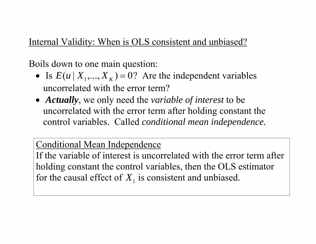
Internal Validity: When is OLS consistent and unbiased? Boils down to one main question: • Is 0),...,|( 1 =KXXuE ? Are the independent variables

uncorrelated with the error term? • Actually, we only need the variable of interest to be

uncorrelated with the error term after holding constant the control variables. Called conditional mean independence.

Conditional Mean Independence If the variable of interest is uncorrelated with the error term after holding constant the control variables, then the OLS estimator for the causal effect of 1X is consistent and unbiased.

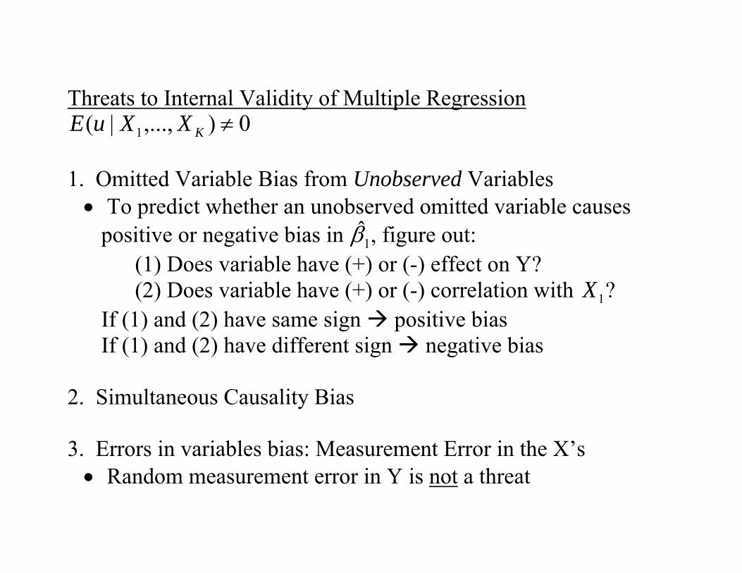
Threats to Internal Validity of Multiple Regression 0),...,|( 1 ≠KXXuE

1. Omitted Variable Bias from Unobserved Variables • To predict whether an unobserved omitted variable causes

positive or negative bias in 1̂β , figure out: (1) Does variable have (+) or (-) effect on Y? (2) Does variable have (+) or (-) correlation with 1X ?

If (1) and (2) have same sign positive bias If (1) and (2) have different sign negative bias

2. Simultaneous Causality Bias 3. Errors in variables bias: Measurement Error in the X’s • Random measurement error in Y is not a threat

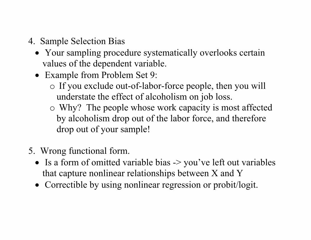
4. Sample Selection Bias • Your sampling procedure systematically overlooks certain

values of the dependent variable. • Example from Problem Set 9:

o If you exclude out-of-labor-force people, then you will understate the effect of alcoholism on job loss.

o Why? The people whose work capacity is most affected by alcoholism drop out of the labor force, and therefore drop out of your sample!

5. Wrong functional form. • Is a form of omitted variable bias -> you’ve left out variables

that capture nonlinear relationships between X and Y • Correctible by using nonlinear regression or probit/logit.

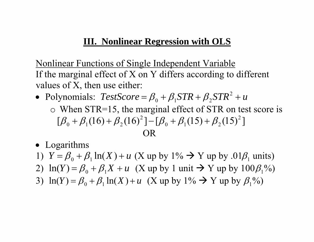
III. Nonlinear Regression with OLS

Nonlinear Functions of Single Independent Variable If the marginal effect of X on Y differs according to different values of X, then use either: • Polynomials: uSTRSTRTestScore +++= 2

210 βββ o When STR=15, the marginal effect of STR on test score is

])15()15([])16()16([ 2210

2210 ββββββ ++−++

OR • Logarithms 1) uXY ++= )ln(10 ββ (X up by 1% Y up by 101. β units) 2) uXY ++= 10)ln( ββ (X up by 1 unit Y up by 100 1β %) 3) uXY ++= )ln()ln( 10 ββ (X up by 1% Y up by 1β %)

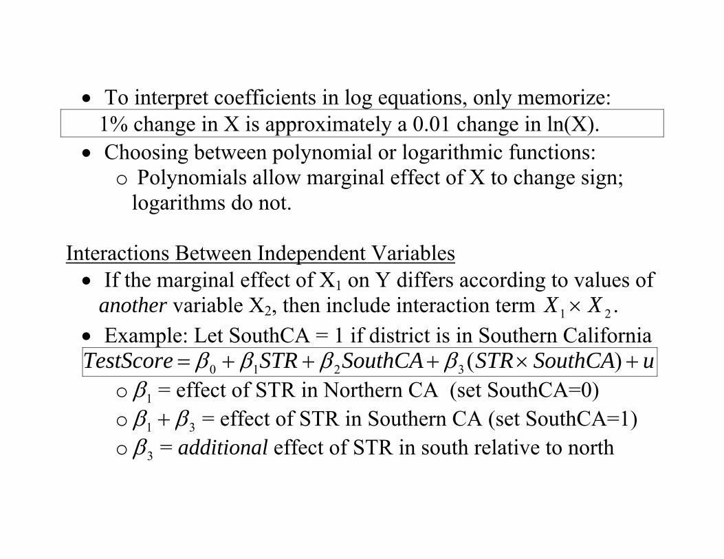
• To interpret coefficients in log equations, only memorize: 1% change in X is approximately a 0.01 change in ln(X). • Choosing between polynomial or logarithmic functions:

o Polynomials allow marginal effect of X to change sign; logarithms do not.

Interactions Between Independent Variables • If the marginal effect of X1 on Y differs according to values of

another variable X2, then include interaction term 21 XX × . • Example: Let SouthCA = 1 if district is in Southern California

uSouthCASTRSouthCASTRTestScore +×+++= )(3210 ββββ o 1β = effect of STR in Northern CA (set SouthCA=0) o 31 ββ + = effect of STR in Southern CA (set SouthCA=1) o 3β = additional effect of STR in south relative to north

IV. Panel Data Regression Cross-sectional data is a snapshot of n entities and panel data is a sequence of snapshots over time. We describe panel data by using two subscripts: often i for entities (individuals, firms, states, etc.) and t for time. N entities each time can be different or same. If follows up the same entities over time. We often call it longitudinal data. In a panel setting the regression error often has the form

itiit uerror += α Regarding the forms of error term, there are three different situations we handle differently

• iα is zero. For example, if we have different car models for each year during 5-year period and pool them together, there is no common component across time. The pooled data (stack data over time) OLS can give us unbiased estimates.

• iα is not zero, and it is correlated with X, we can use fixed-effect methodology. When we

only have two-time period, fixed-effect is equivalent with differencing strategy (also called “before and after” methodology)

• iα is not zero, but it is not correlated with X. Not really covered in this course. Random

Effects or Clustered SE

Note that in a fixed effects model it is possible that 0),( 1,, ≠−titi uuCov In this case we should use clustered standard errors even though we have included fixed effects. We focus on the second situation ( iα is not zero, and it is correlated with X). The goal is to deal with the omitted factor iα that is constant within an entity but doesn’t vary over time. (example: a persons gender, race, or country of birth does not change over time) *A fixed effects regression uses the variation within an entity to make identification in order to control for unobserved differences across entities, rather than comparing apples and oranges. (Ex: compare Arizona today to Arizona tomorrow rather than comparing Arizona to New York)

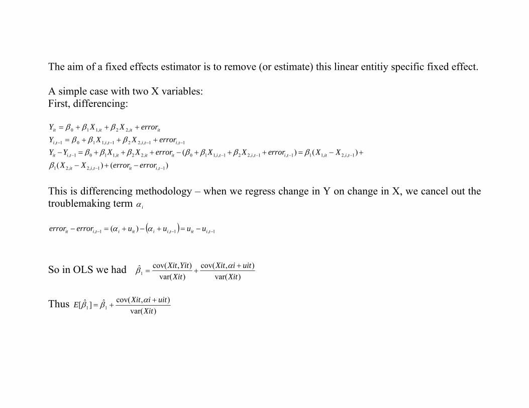
The aim of a fixed effects estimator is to remove (or estimate) this linear entitiy specific fixed effect. A simple case with two X variables: First, differencing:

itititit errorXXY +++= ,22,110 βββ 1,1,,221,,1101, −−−− +++= titititi errorXXY βββ

, 1 0 1 1, 2 2, 0 1 1, , 1 2 2, , 1 , 1 1 1, 2, , 1

1 2, 2, , 1 , 1

( ) ( )( ) ( )

it i t it it it i t i t i t it i t

it i t it i t

Y Y X X error X X error X XX X error error

β β β β β β β

β− − − − −

− −

− = + + + − + + + = − +

− + −

This is differencing methodology – when we regress change in Y on change in X, we cancel out the troublemaking term iα

( ) 1,1,1, )( −−− −=+−+=− tiittiiititiit uuuuerrorerror αα So in OLS we had

)var(),cov(

)var(),cov(ˆ

1 XituitiXit

XitYitXit +

+=αβ

Thus

)var(),cov(ˆ]ˆ[ 11 Xit

uitiXitE ++=

αββ

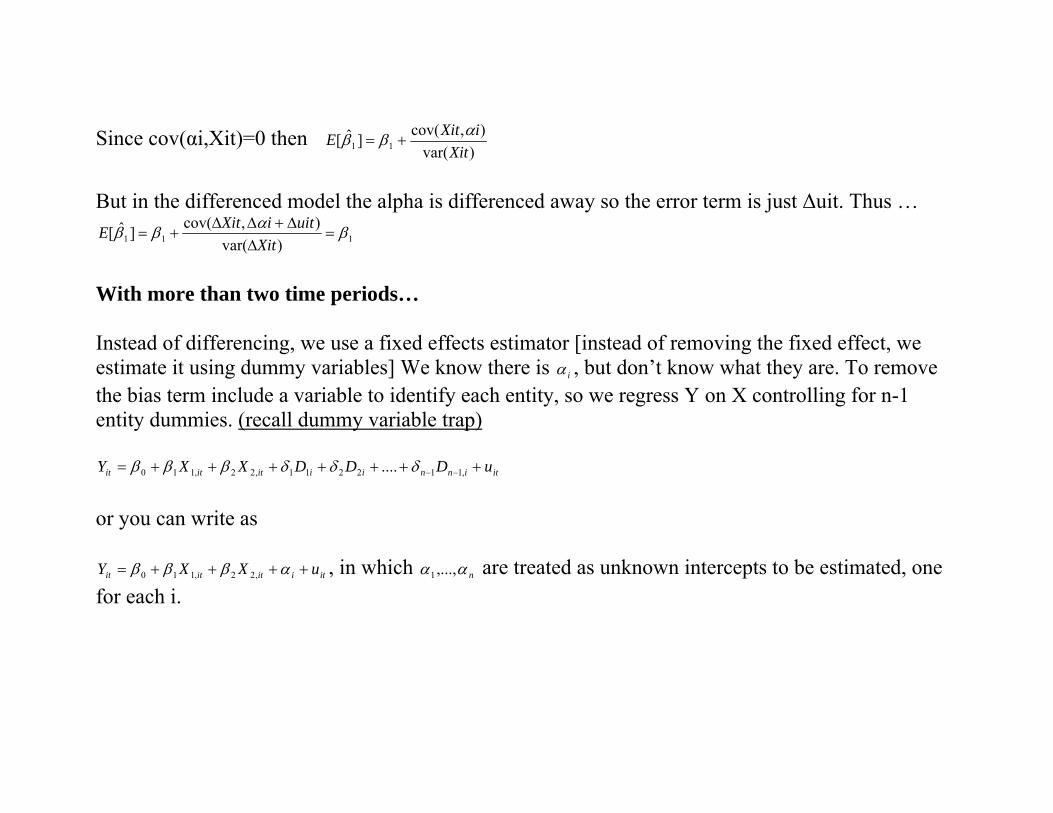
Since cov(αi,Xit)=0 then )var(

),cov(]ˆ[ 11 XitiXitE αββ +=

But in the differenced model the alpha is differenced away so the error term is just ∆uit. Thus …

111 )var(),cov(]ˆ[ βαββ =

∆∆+∆∆

+=Xit

uitiXitE

With more than two time periods… Instead of differencing, we use a fixed effects estimator [instead of removing the fixed effect, we estimate it using dummy variables] We know there is iα , but don’t know what they are. To remove the bias term include a variable to identify each entity, so we regress Y on X controlling for n-1 entity dummies. (recall dummy variable trap)

itinniiititit uDDDXXY +++++++= −− ,112211,22,110 .... δδδβββ or you can write as

itiititit uXXY ++++= αβββ ,22,110 , in which nαα ,...,1 are treated as unknown intercepts to be estimated, one for each i.

For example, if i stands for state, the interpretation of iα is a state-specific intercept. If the dependent variable is crime, then a large iα means that state I has a lot of crime on average, and a low iα means state I has less crime than average. Also time fixed effects are useful in dealing with omitted variables that don’t vary across entities yet vary over time. *Note: One should use an F-test in order to determine the significance of the dummy variables. In summary, the fixed effects regression model:

( ) ( )0 1 1 2 2 1 1 2 2 1 1 1 1 2 2 1 1... ... ( ... )it it it k kit N N T T itY X X X D D D B B B uβ β β β γ γ γ δ δ δ− − − −= + + + + + + + + + + + + + for 1,2,...,i N= and 1,2,...,t T=

2itX means variable 2X for individual i at time t . 1 2 1, ,... ND D D − are the individual dummies and the iγ coefficients are individual fixed effects. 1 2 1, ,... TB B B − are the time dummies and the tδ coefficients are time fixed effects.

You use 1N − individual dummies and 1T − time dummies to avoid perfect multicollinearity. Also, you cannot use any variable that stays constant for each individual or that varies linearly with time.

Sample Question: We have data for 366 student-athletes from a large university for fall and spring semesters during one academic year. The research question is this: Do athletes perform more poorly in school during the semester their sport is in season? Y: GPA X’s: spring, SAT, hsperc(high school percentile), female, black, white, frstsem, season We pool data across semesters and use OLS to get the following estimation: GPA=-1.75-0.058spring + 0.0017sat-0.0087 hsperc +0.35female -0.254black+0.023white -0.027 season standard errors for each coefficients are 0.35, 0.48, 0.00015, 0.001, 0.052, 0.123, 0.117, and 0.0049.

(1) Explain the coefficient of season. (Other things fixed, an athlete’s team GPA is about 0.27 points lower when his/her sport is in season. The estimate is statistically significant. )

Now suppose ability is correlated with season, then you can use fixed effects to solve the problem (to control for the unobserved ability).

(2) Now if we used a fixed effects estimator, which variables will drop out?

(variables that don’t vary over time will drop out, including sat, hsperc, female, black, and white).

(3) If we simply included a dummy variable for each student will the standard errors in

part(2) be valid? (there may exist serial correlation between the error terms for each individual)

(4) What can we do to address the problem in part(3)? The issue in part(3) is that the error term may be correlated across time. The best way to address this is to use HAC standard errors. (5) Can you think of one potential internal threat after using differencing strategy (or

individual fixed effect) – individual fixed effect deals with individual-specific and time-constant omitted variable, but one or more potentially important, time-varying variables might be omitted from the analysis. This will bias our estimation. One example is the measure of course load. If some fraction of student-athletes take a lighter load during the season, then term GPA may tend to be higher, other things equal. This would bias the results away from finding an effect of season on term GPA.

V. Binary Dependent Variables

1.1 Linear Probability Model 0 1i i iY X uβ β= + + Yi: 0 or 1

1β = change in probability that Y = 1 for a given ∆x:

1β = Pr( 1| ) Pr( 1| )Y X x x Y X xx

= = + ∆ − = =∆

Advantages: simple to estimate and to interpret inference is the same as for multiple regression (need heteroskedasticity robust standard

errors) Disadvantages:

Does it make sense that the probability should be linear in X? Predicted probabilities can be <0 or >1!

Why the probability is linear in X? How about an “S-curve”, then it can satisfy: • 0 ≤ Pr(Y = 1|X) ≤ 1 for all X • Pr(Y = 1|X) to be increasing in X (for β1>0)

Solutions: Probit or Logit Model: Non-linear function bounded between zero and one

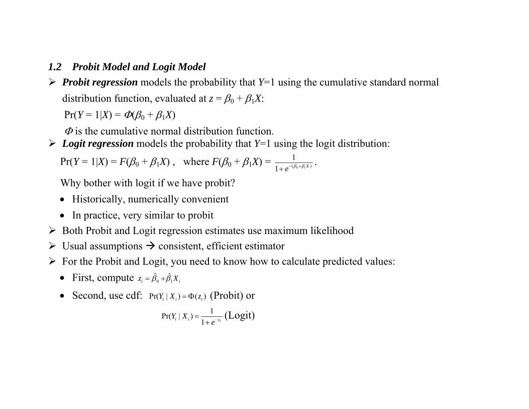
1.2 Probit Model and Logit Model Probit regression models the probability that Y=1 using the cumulative standard normal

distribution function, evaluated at z = β0 + β1X: Pr(Y = 1|X) = Φ(β0 + β1X) Φ is the cumulative normal distribution function.

Logit regression models the probability that Y=1 using the logit distribution:

Pr(Y = 1|X) = F(β0 + β1X) , where F(β0 + β1X) = 0 1( )

11 Xe β β− ++

.

Why bother with logit if we have probit? • Historically, numerically convenient • In practice, very similar to probit

Both Probit and Logit regression estimates use maximum likelihood Usual assumptions consistent, efficient estimator For the Probit and Logit, you need to know how to calculate predicted values: • First, compute 0

ˆiz β= 1̂ iXβ+

• Second, use cdf: Pr( | ) ( )i i iY X z= Φ (Probit) or 1Pr( | )

1 ii i zY Xe−=

+(Logit)

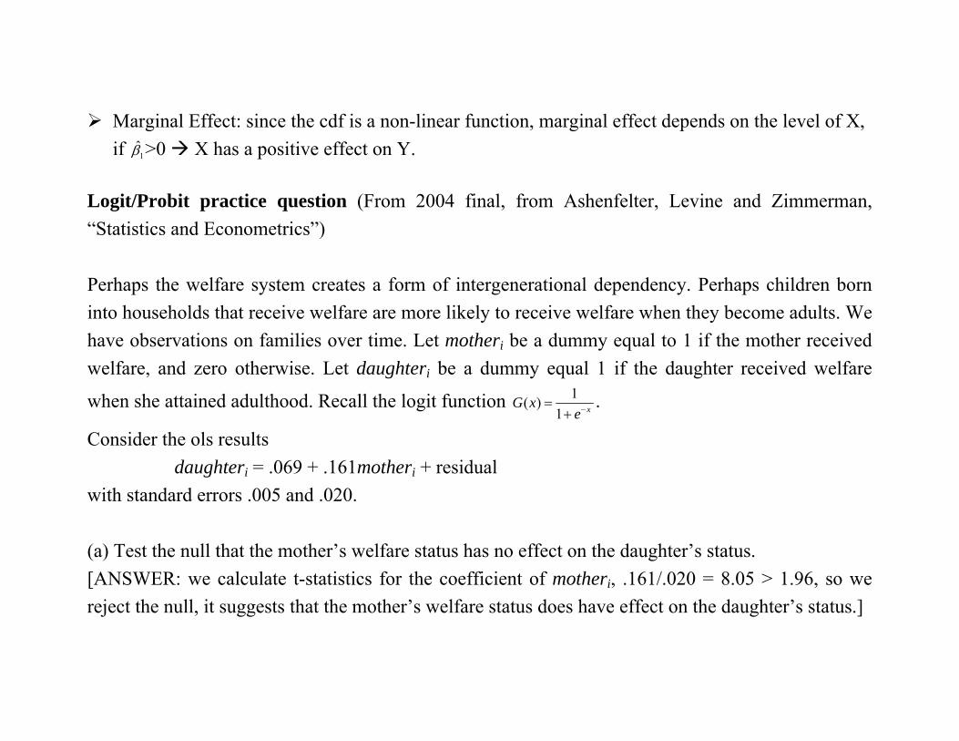
Marginal Effect: since the cdf is a non-linear function, marginal effect depends on the level of X, if 1̂β >0 X has a positive effect on Y.

Logit/Probit practice question (From 2004 final, from Ashenfelter, Levine and Zimmerman, “Statistics and Econometrics”) Perhaps the welfare system creates a form of intergenerational dependency. Perhaps children born into households that receive welfare are more likely to receive welfare when they become adults. We have observations on families over time. Let motheri be a dummy equal to 1 if the mother received welfare, and zero otherwise. Let daughteri be a dummy equal 1 if the daughter received welfare

when she attained adulthood. Recall the logit function 1( )1 xG x

e−=+

.

Consider the ols results daughteri = .069 + .161motheri + residual with standard errors .005 and .020. (a) Test the null that the mother’s welfare status has no effect on the daughter’s status. [ANSWER: we calculate t-statistics for the coefficient of motheri, .161/.020 = 8.05 > 1.96, so we reject the null, it suggests that the mother’s welfare status does have effect on the daughter’s status.]

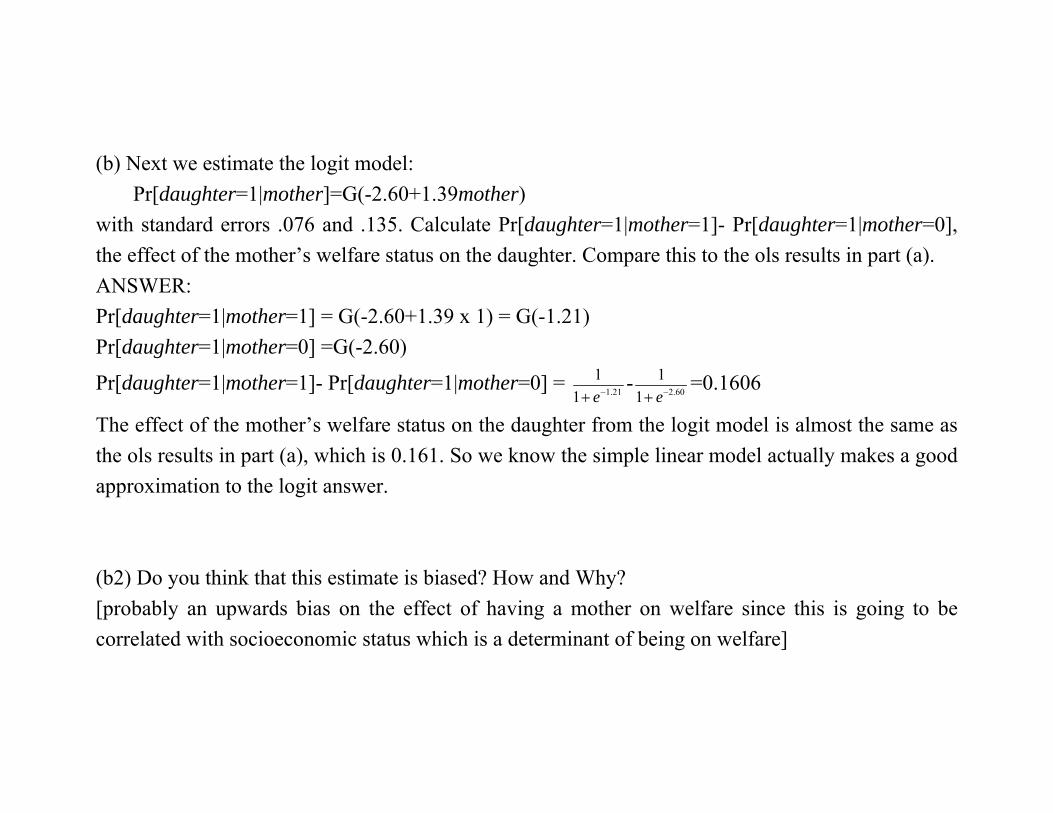
(b) Next we estimate the logit model: Pr[daughter=1|mother]=G(-2.60+1.39mother) with standard errors .076 and .135. Calculate Pr[daughter=1|mother=1]- Pr[daughter=1|mother=0], the effect of the mother’s welfare status on the daughter. Compare this to the ols results in part (a). ANSWER: Pr[daughter=1|mother=1] = G(-2.60+1.39 x 1) = G(-1.21) Pr[daughter=1|mother=0] =G(-2.60)

Pr[daughter=1|mother=1]- Pr[daughter=1|mother=0] = 1.21

11 e−+

- 2.60

11 e−+

=0.1606

The effect of the mother’s welfare status on the daughter from the logit model is almost the same as the ols results in part (a), which is 0.161. So we know the simple linear model actually makes a good approximation to the logit answer. (b2) Do you think that this estimate is biased? How and Why? [probably an upwards bias on the effect of having a mother on welfare since this is going to be correlated with socioeconomic status which is a determinant of being on welfare]

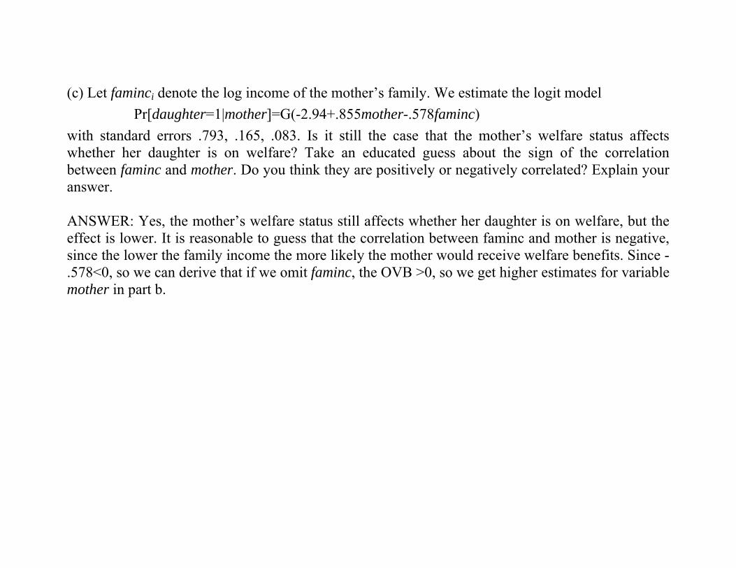
(c) Let faminci denote the log income of the mother’s family. We estimate the logit model Pr[daughter=1|mother]=G(-2.94+.855mother-.578faminc) with standard errors .793, .165, .083. Is it still the case that the mother’s welfare status affects whether her daughter is on welfare? Take an educated guess about the sign of the correlation between faminc and mother. Do you think they are positively or negatively correlated? Explain your answer. ANSWER: Yes, the mother’s welfare status still affects whether her daughter is on welfare, but the effect is lower. It is reasonable to guess that the correlation between faminc and mother is negative, since the lower the family income the more likely the mother would receive welfare benefits. Since -.578<0, so we can derive that if we omit faminc, the OVB >0, so we get higher estimates for variable mother in part b.

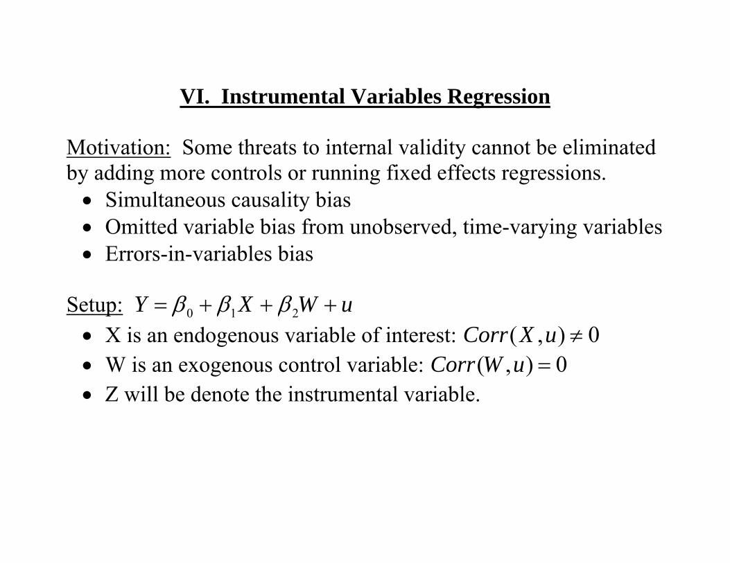
VI. Instrumental Variables Regression

Motivation: Some threats to internal validity cannot be eliminated by adding more controls or running fixed effects regressions. • Simultaneous causality bias • Omitted variable bias from unobserved, time-varying variables • Errors-in-variables bias

Setup: uWXY +++= 210 βββ • X is an endogenous variable of interest: 0),( ≠uXCorr • W is an exogenous control variable: 0),( =uWCorr • Z will be denote the instrumental variable.

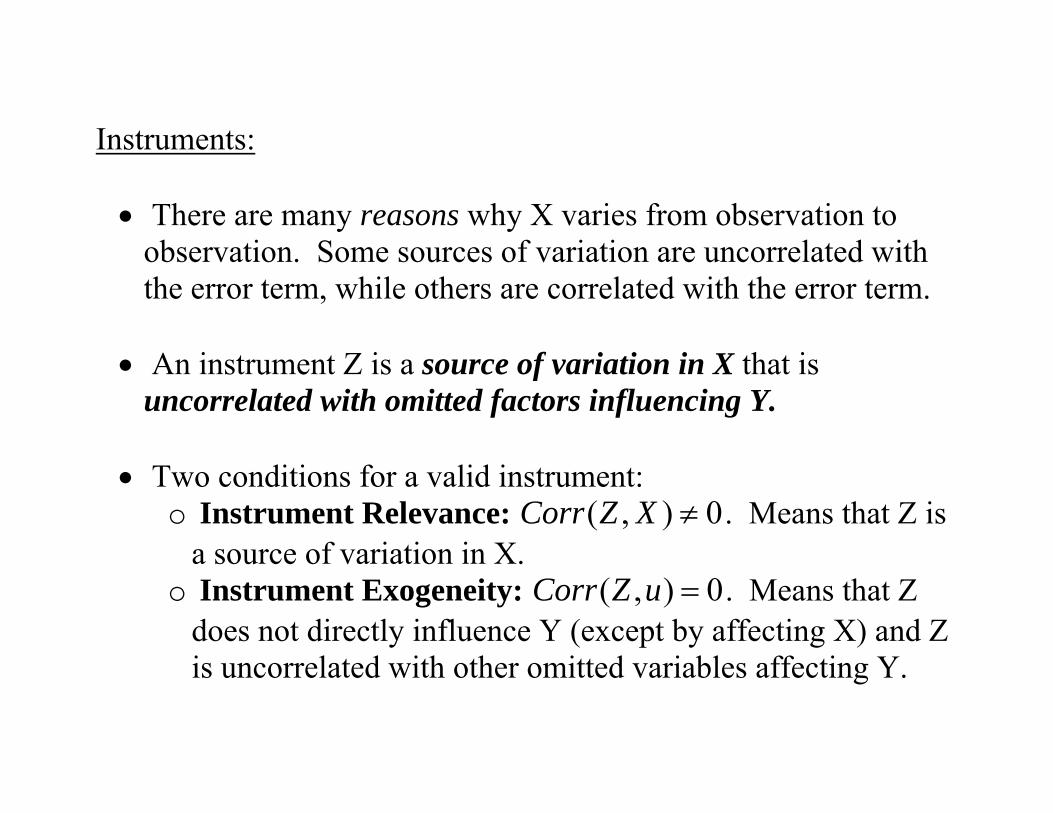
Instruments: • There are many reasons why X varies from observation to

observation. Some sources of variation are uncorrelated with the error term, while others are correlated with the error term.

• An instrument Z is a source of variation in X that is

uncorrelated with omitted factors influencing Y. • Two conditions for a valid instrument:

o Instrument Relevance: 0),( ≠XZCorr . Means that Z is a source of variation in X.

o Instrument Exogeneity: 0),( =uZCorr . Means that Z does not directly influence Y (except by affecting X) and Z is uncorrelated with other omitted variables affecting Y.

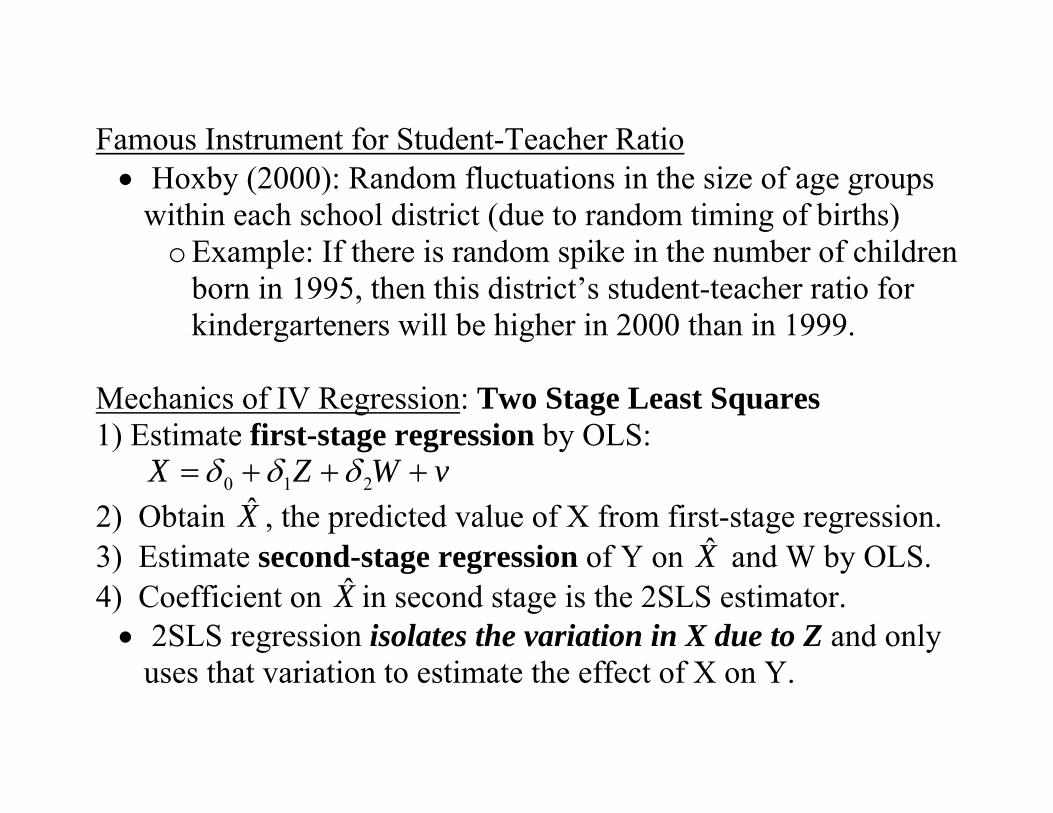
Famous Instrument for Student-Teacher Ratio • Hoxby (2000): Random fluctuations in the size of age groups

within each school district (due to random timing of births) o Example: If there is random spike in the number of children

born in 1995, then this district’s student-teacher ratio for kindergarteners will be higher in 2000 than in 1999.

Mechanics of IV Regression: Two Stage Least Squares 1) Estimate first-stage regression by OLS:

vWZX +++= 210 δδδ 2) Obtain X̂ , the predicted value of X from first-stage regression. 3) Estimate second-stage regression of Y on X̂ and W by OLS. 4) Coefficient on X̂ in second stage is the 2SLS estimator. • 2SLS regression isolates the variation in X due to Z and only

uses that variation to estimate the effect of X on Y.

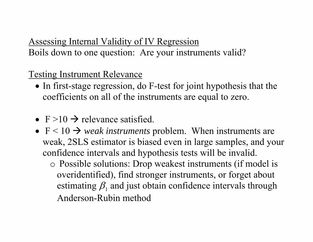
Assessing Internal Validity of IV Regression Boils down to one question: Are your instruments valid?

Testing Instrument Relevance • In first-stage regression, do F-test for joint hypothesis that the

coefficients on all of the instruments are equal to zero. • F >10 relevance satisfied. • F < 10 weak instruments problem. When instruments are

weak, 2SLS estimator is biased even in large samples, and your confidence intervals and hypothesis tests will be invalid. o Possible solutions: Drop weakest instruments (if model is

overidentified), find stronger instruments, or forget about estimating 1β and just obtain confidence intervals through Anderson-Rubin method

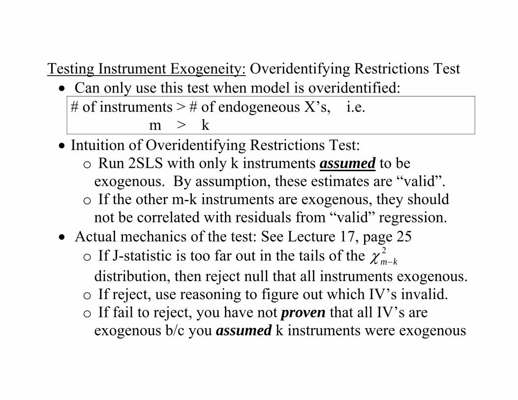
Testing Instrument Exogeneity: Overidentifying Restrictions Test • Can only use this test when model is overidentified:

# of instruments > # of endogeneous X’s, i.e. m > k

• Intuition of Overidentifying Restrictions Test: o Run 2SLS with only k instruments assumed to be

exogenous. By assumption, these estimates are “valid”. o If the other m-k instruments are exogenous, they should

not be correlated with residuals from “valid” regression. • Actual mechanics of the test: See Lecture 17, page 25

o If J-statistic is too far out in the tails of the 2km−χ

distribution, then reject null that all instruments exogenous. o If reject, use reasoning to figure out which IV’s invalid. o If fail to reject, you have not proven that all IV’s are

exogenous b/c you assumed k instruments were exogenous

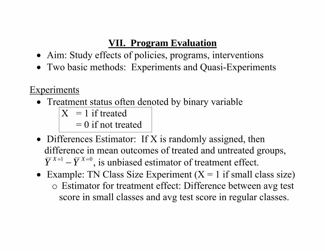
VII. Program Evaluation • Aim: Study effects of policies, programs, interventions • Two basic methods: Experiments and Quasi-Experiments

Experiments • Treatment status often denoted by binary variable

X = 1 if treated = 0 if not treated

• Differences Estimator: If X is randomly assigned, then difference in mean outcomes of treated and untreated groups,

01 == − XX YY , is unbiased estimator of treatment effect. • Example: TN Class Size Experiment (X = 1 if small class size)

o Estimator for treatment effect: Difference between avg test score in small classes and avg test score in regular classes.

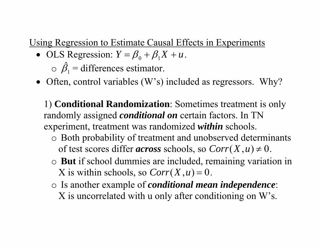
Using Regression to Estimate Causal Effects in Experiments • OLS Regression: uXY ++= 10 ββ .

o 1̂β = differences estimator. • Often, control variables (W’s) included as regressors. Why?

1) Conditional Randomization: Sometimes treatment is only randomly assigned conditional on certain factors. In TN experiment, treatment was randomized within schools. o Both probability of treatment and unobserved determinants

of test scores differ across schools, so 0),( ≠uXCorr . o But if school dummies are included, remaining variation in

X is within schools, so 0),( =uXCorr . o Is another example of conditional mean independence:

X is uncorrelated with u only after conditioning on W’s.

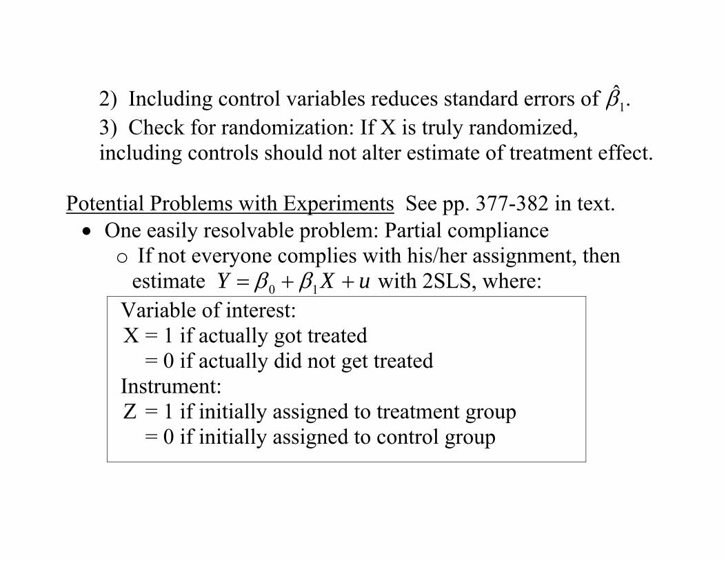
2) Including control variables reduces standard errors of 1̂β . 3) Check for randomization: If X is truly randomized, including controls should not alter estimate of treatment effect.

Potential Problems with Experiments See pp. 377-382 in text. • One easily resolvable problem: Partial compliance

o If not everyone complies with his/her assignment, then estimate uXY ++= 10 ββ with 2SLS, where:

Variable of interest: X = 1 if actually got treated = 0 if actually did not get treated Instrument:

Z = 1 if initially assigned to treatment group = 0 if initially assigned to control group

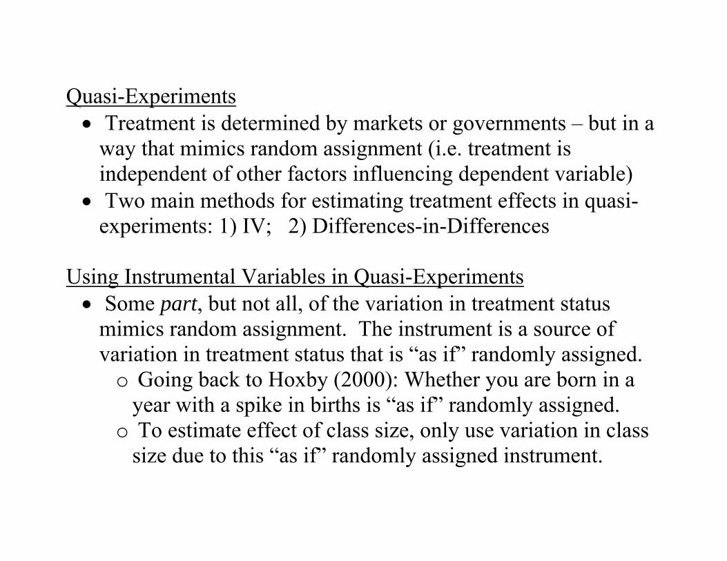
Quasi-Experiments • Treatment is determined by markets or governments – but in a

way that mimics random assignment (i.e. treatment is independent of other factors influencing dependent variable)

• Two main methods for estimating treatment effects in quasi-experiments: 1) IV; 2) Differences-in-Differences

Using Instrumental Variables in Quasi-Experiments • Some part, but not all, of the variation in treatment status

mimics random assignment. The instrument is a source of variation in treatment status that is “as if” randomly assigned. o Going back to Hoxby (2000): Whether you are born in a

year with a spike in births is “as if” randomly assigned. o To estimate effect of class size, only use variation in class

size due to this “as if” randomly assigned instrument.

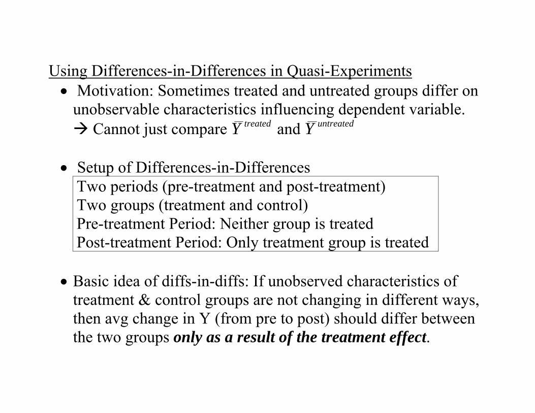
Using Differences-in-Differences in Quasi-Experiments • Motivation: Sometimes treated and untreated groups differ on

unobservable characteristics influencing dependent variable. Cannot just compare treatedY and untreatedY

• Setup of Differences-in-Differences

Two periods (pre-treatment and post-treatment) Two groups (treatment and control) Pre-treatment Period: Neither group is treated Post-treatment Period: Only treatment group is treated

• Basic idea of diffs-in-diffs: If unobserved characteristics of

treatment & control groups are not changing in different ways, then avg change in Y (from pre to post) should differ between the two groups only as a result of the treatment effect.

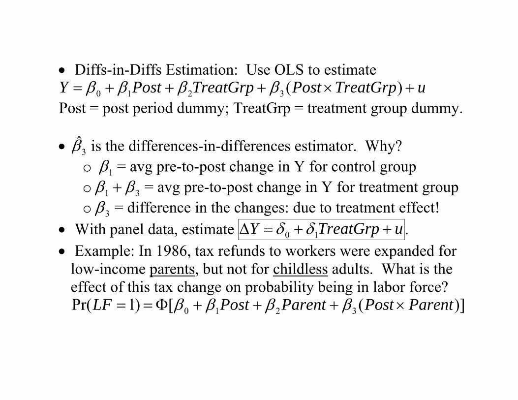
• Diffs-in-Diffs Estimation: Use OLS to estimate uTreatGrpPostTreatGrpPostY +×+++= )(3210 ββββ

Post = post period dummy; TreatGrp = treatment group dummy. • 3β̂ is the differences-in-differences estimator. Why?

o 1β = avg pre-to-post change in Y for control group o 31 ββ + = avg pre-to-post change in Y for treatment group o 3β = difference in the changes: due to treatment effect!

• With panel data, estimate uTreatGrpY ++=∆ 10 δδ . • Example: In 1986, tax refunds to workers were expanded for

low-income parents, but not for childless adults. What is the effect of this tax change on probability being in labor force?

)]([)1Pr( 3210 ParentPostParentPostLF ×+++Φ== ββββ

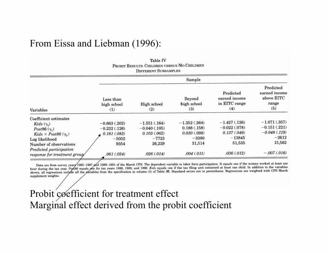
From Eissa and Liebman (1996):

Probit coefficient for treatment effect Marginal effect derived from the probit coefficient

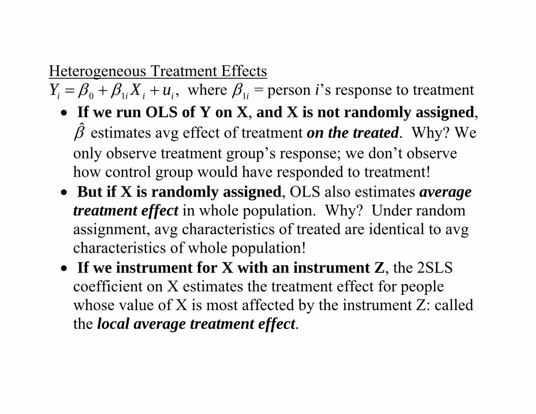
Heterogeneous Treatment Effects iiii uXY ++= 10 ββ , where i1β = person i’s response to treatment

• If we run OLS of Y on X, and X is not randomly assigned, β̂ estimates avg effect of treatment on the treated. Why? We only observe treatment group’s response; we don’t observe how control group would have responded to treatment!

• But if X is randomly assigned, OLS also estimates average treatment effect in whole population. Why? Under random assignment, avg characteristics of treated are identical to avg characteristics of whole population!

• If we instrument for X with an instrument Z, the 2SLS coefficient on X estimates the treatment effect for people whose value of X is most affected by the instrument Z: called the local average treatment effect.

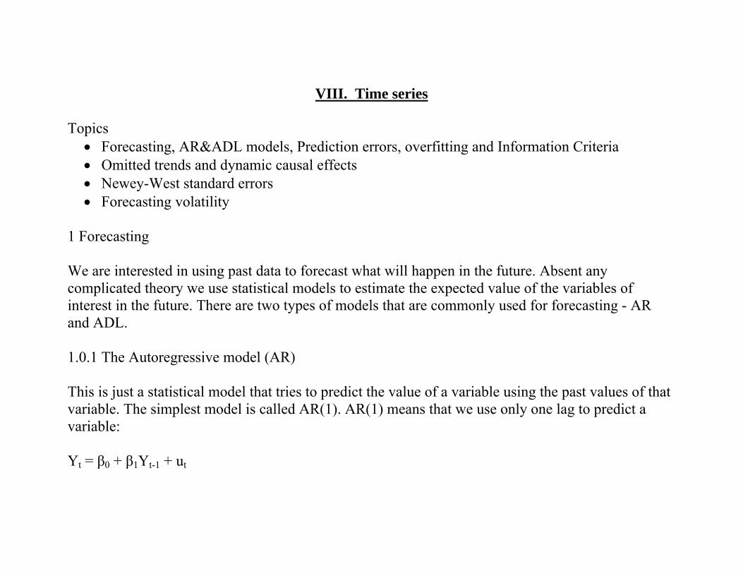
VIII. Time series Topics

• Forecasting, AR&ADL models, Prediction errors, overfitting and Information Criteria • Omitted trends and dynamic causal effects • Newey-West standard errors • Forecasting volatility

1 Forecasting We are interested in using past data to forecast what will happen in the future. Absent any complicated theory we use statistical models to estimate the expected value of the variables of interest in the future. There are two types of models that are commonly used for forecasting - AR and ADL. 1.0.1 The Autoregressive model (AR) This is just a statistical model that tries to predict the value of a variable using the past values of that variable. The simplest model is called AR(1). AR(1) means that we use only one lag to predict a variable: Yt = β0 + β1Yt-1 + ut

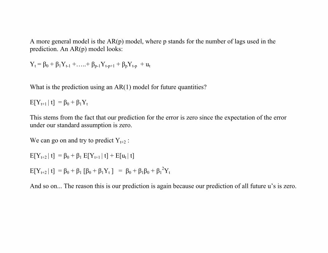
A more general model is the AR(p) model, where p stands for the number of lags used in the prediction. An AR(p) model looks: Yt = β0 + β1Yt-1 +…..+ βp-1Yt-p+1 + βpYt-p + ut What is the prediction using an AR(1) model for future quantities? E[Yt+1 | t] = β0 + β1Yt This stems from the fact that our prediction for the error is zero since the expectation of the error under our standard assumption is zero. We can go on and try to predict Yt+2 : E[Yt+2 | t] = β0 + β1 E[Yt+1 | t] + E[ut | t] E[Yt+2 | t] = β0 + β1 [β0 + β1Yt ] = β0 + β1β0 + β1

2Yt And so on... The reason this is our prediction is again because our prediction of all future u’s is zero.

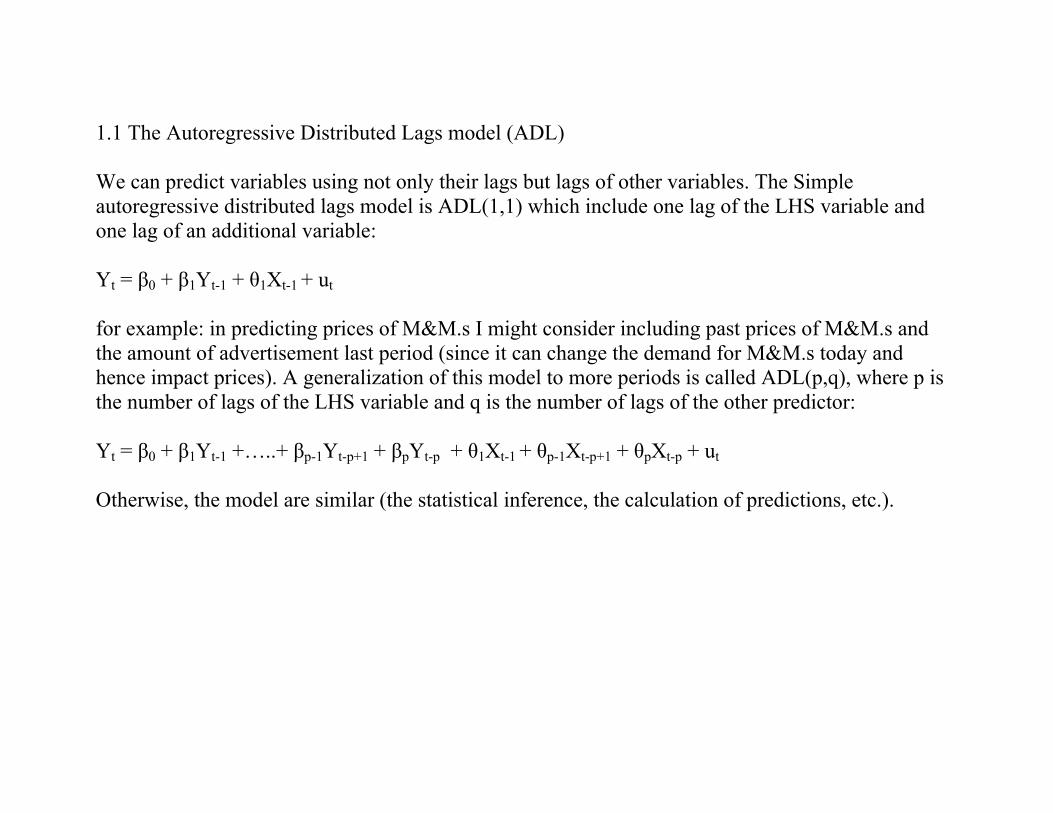
1.1 The Autoregressive Distributed Lags model (ADL) We can predict variables using not only their lags but lags of other variables. The Simple autoregressive distributed lags model is ADL(1,1) which include one lag of the LHS variable and one lag of an additional variable: Yt = β0 + β1Yt-1 + θ1Xt-1 + ut for example: in predicting prices of M&M.s I might consider including past prices of M&M.s and the amount of advertisement last period (since it can change the demand for M&M.s today and hence impact prices). A generalization of this model to more periods is called ADL(p,q), where p is the number of lags of the LHS variable and q is the number of lags of the other predictor: Yt = β0 + β1Yt-1 +…..+ βp-1Yt-p+1 + βpYt-p + θ1Xt-1 + θp-1Xt-p+1 + θpXt-p + ut Otherwise, the model are similar (the statistical inference, the calculation of predictions, etc.).

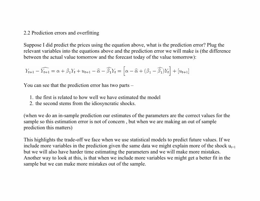
2.2 Prediction errors and overfitting Suppose I did predict the prices using the equation above, what is the prediction error? Plug the relevant variables into the equations above and the prediction error we will make is (the difference between the actual value tomorrow and the forecast today of the value tomorrow):

You can see that the prediction error has two parts –

1. the first is related to how well we have estimated the model 2. the second stems from the idiosyncratic shocks.

(when we do an in-sample prediction our estimates of the parameters are the correct values for the sample so this estimation error is not of concern , but when we are making an out of sample prediction this matters) This highlights the trade-off we face when we use statistical models to predict future values. If we include more variables in the prediction given the same data we might explain more of the shock ut+1 but we will also have harder time estimating the parameters and we will make more mistakes. Another way to look at this, is that when we include more variables we might get a better fit in the sample but we can make more mistakes out of the sample.

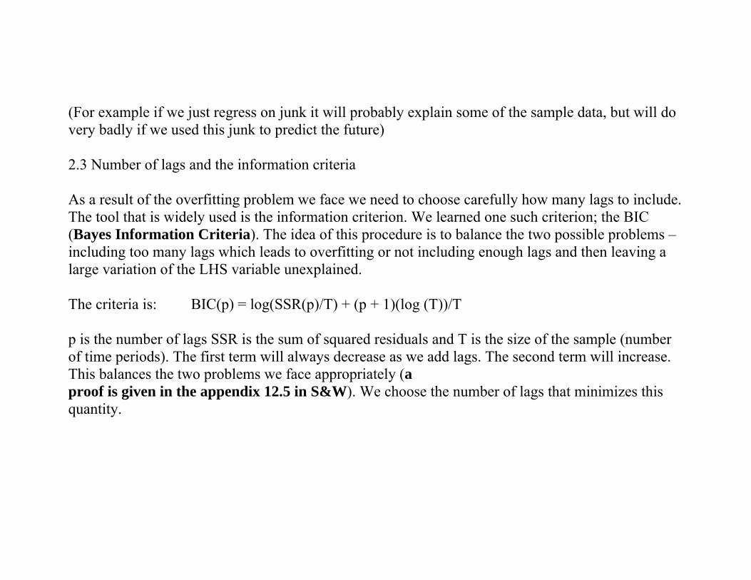
(For example if we just regress on junk it will probably explain some of the sample data, but will do very badly if we used this junk to predict the future) 2.3 Number of lags and the information criteria As a result of the overfitting problem we face we need to choose carefully how many lags to include. The tool that is widely used is the information criterion. We learned one such criterion; the BIC (Bayes Information Criteria). The idea of this procedure is to balance the two possible problems – including too many lags which leads to overfitting or not including enough lags and then leaving a large variation of the LHS variable unexplained. The criteria is: BIC(p) = log(SSR(p)/T) + (p + 1)(log (T))/T p is the number of lags SSR is the sum of squared residuals and T is the size of the sample (number of time periods). The first term will always decrease as we add lags. The second term will increase. This balances the two problems we face appropriately (a proof is given in the appendix 12.5 in S&W). We choose the number of lags that minimizes this quantity.

3 Omitted trends and dynamic causal effects (A side note) One phenomenon in time series data is that we might observe a high correlation between two time series but there is no actual causal effect in the relationship between the two variables. The problem is that there is some trend in the series over time due to factors that are unrelated. However, when we measure the correlation we find a strikingly strong relationship (which can quickly disappear with more data). This is called spurious regressions and we need to be aware of this phenomenon. The way to address this problem is to add a time trend and try to see if the variables are related to each other when we actually look at only the variation around the trend. Dynamic Causal Effects When we consider the relationship between two series over time, we might not only be interested in the contemporaneous relationship but also in how past values of other variables impact the LHS variable of interest (like an ADL model but without the autoregressive part and with causality and not forecasting in mind). For example, a model with dynamic causal effects is: Yt = β0 + β1Xt-1 + β2Xt-2 + β3Xt-3 + ut

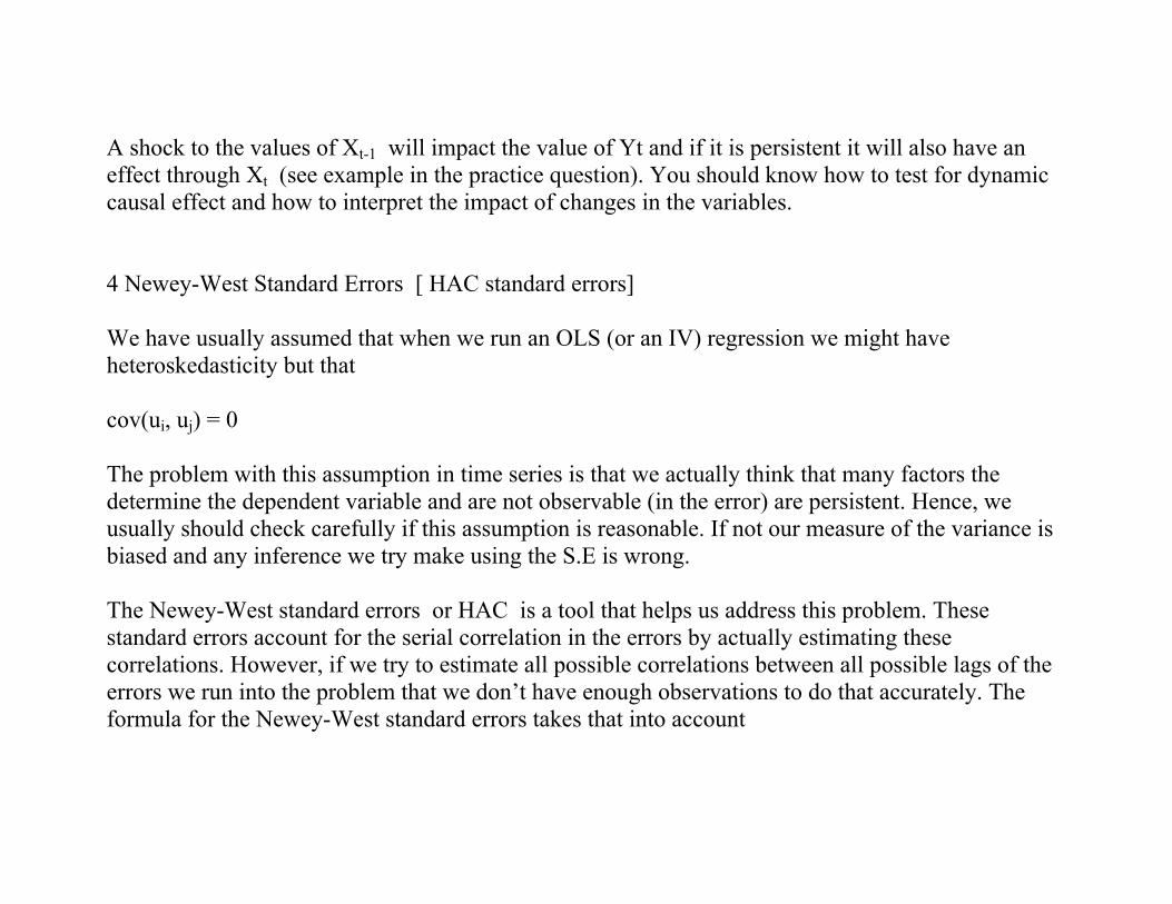
A shock to the values of Xt-1 will impact the value of Yt and if it is persistent it will also have an effect through Xt (see example in the practice question). You should know how to test for dynamic causal effect and how to interpret the impact of changes in the variables. 4 Newey-West Standard Errors [ HAC standard errors] We have usually assumed that when we run an OLS (or an IV) regression we might have heteroskedasticity but that cov(ui, uj) = 0 The problem with this assumption in time series is that we actually think that many factors the determine the dependent variable and are not observable (in the error) are persistent. Hence, we usually should check carefully if this assumption is reasonable. If not our measure of the variance is biased and any inference we try make using the S.E is wrong. The Newey-West standard errors or HAC is a tool that helps us address this problem. These standard errors account for the serial correlation in the errors by actually estimating these correlations. However, if we try to estimate all possible correlations between all possible lags of the errors we run into the problem that we don’t have enough observations to do that accurately. The formula for the Newey-West standard errors takes that into account

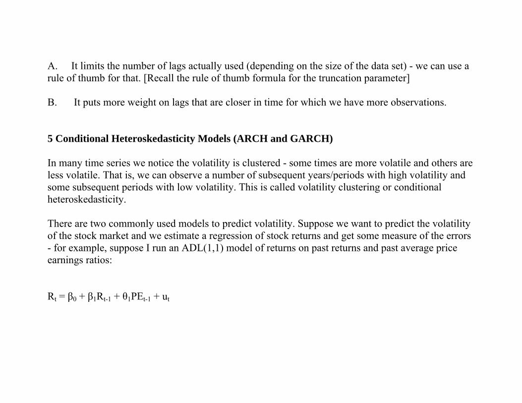
A. It limits the number of lags actually used (depending on the size of the data set) - we can use a rule of thumb for that. [Recall the rule of thumb formula for the truncation parameter] B. It puts more weight on lags that are closer in time for which we have more observations. 5 Conditional Heteroskedasticity Models (ARCH and GARCH) In many time series we notice the volatility is clustered - some times are more volatile and others are less volatile. That is, we can observe a number of subsequent years/periods with high volatility and some subsequent periods with low volatility. This is called volatility clustering or conditional heteroskedasticity. There are two commonly used models to predict volatility. Suppose we want to predict the volatility of the stock market and we estimate a regression of stock returns and get some measure of the errors - for example, suppose I run an ADL(1,1) model of returns on past returns and past average price earnings ratios: Rt = β0 + β1Rt-1 + θ1PEt-1 + ut

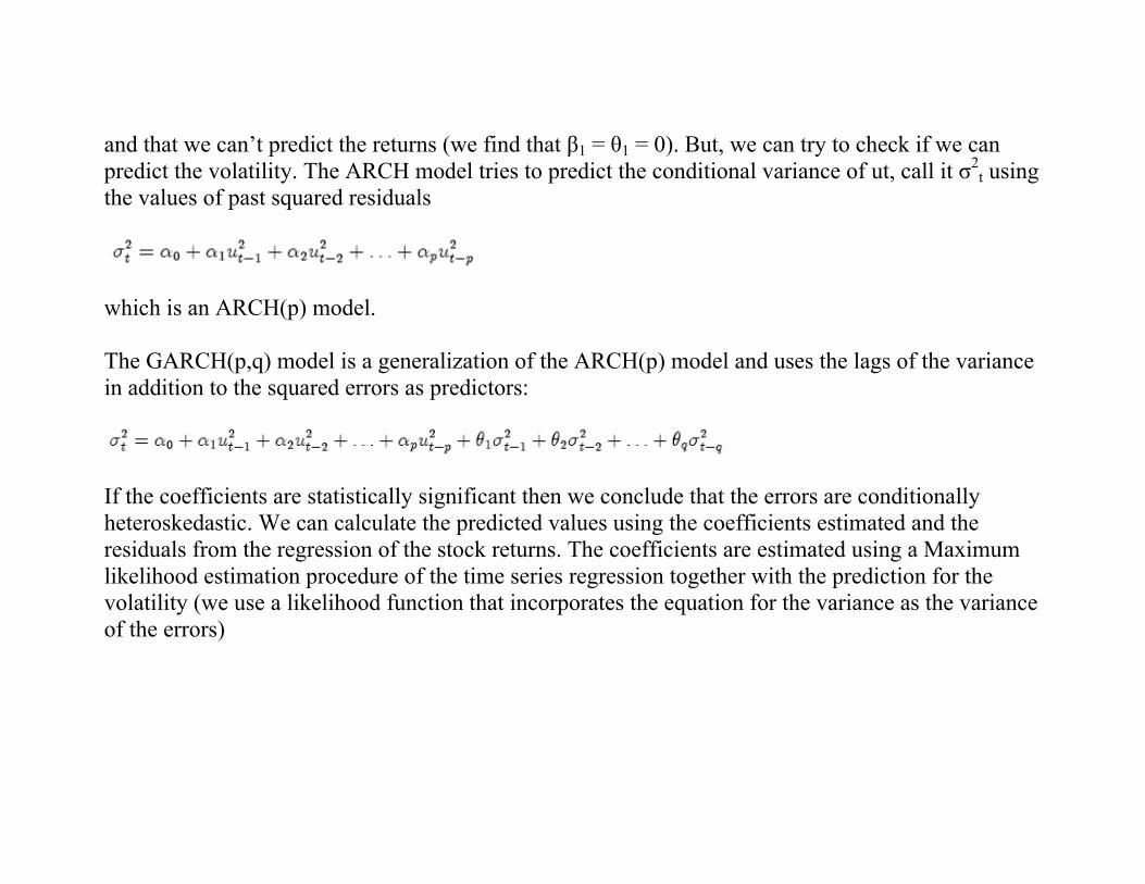
and that we can’t predict the returns (we find that β1 = θ1 = 0). But, we can try to check if we can predict the volatility. The ARCH model tries to predict the conditional variance of ut, call it σ2

t using the values of past squared residuals

which is an ARCH(p) model. The GARCH(p,q) model is a generalization of the ARCH(p) model and uses the lags of the variance in addition to the squared errors as predictors:

If the coefficients are statistically significant then we conclude that the errors are conditionally heteroskedastic. We can calculate the predicted values using the coefficients estimated and the residuals from the regression of the stock returns. The coefficients are estimated using a Maximum likelihood estimation procedure of the time series regression together with the prediction for the volatility (we use a likelihood function that incorporates the equation for the variance as the variance of the errors)

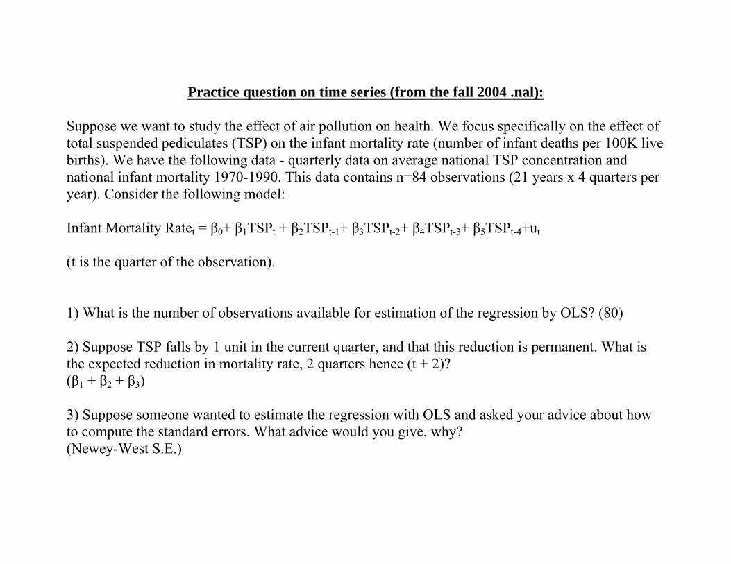
Practice question on time series (from the fall 2004 .nal): Suppose we want to study the effect of air pollution on health. We focus specifically on the effect of total suspended pediculates (TSP) on the infant mortality rate (number of infant deaths per 100K live births). We have the following data - quarterly data on average national TSP concentration and national infant mortality 1970-1990. This data contains n=84 observations (21 years x 4 quarters per year). Consider the following model: Infant Mortality Ratet = β0+ β1TSPt + β2TSPt-1+ β3TSPt-2+ β4TSPt-3+ β5TSPt-4+ut (t is the quarter of the observation). 1) What is the number of observations available for estimation of the regression by OLS? (80) 2) Suppose TSP falls by 1 unit in the current quarter, and that this reduction is permanent. What is the expected reduction in mortality rate, 2 quarters hence (t + 2)? (β1 + β2 + β3) 3) Suppose someone wanted to estimate the regression with OLS and asked your advice about how to compute the standard errors. What advice would you give, why? (Newey-West S.E.)

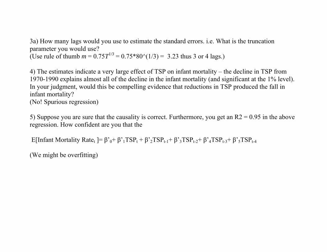
3a) How many lags would you use to estimate the standard errors. i.e. What is the truncation parameter you would use? (Use rule of thumb m = 0.75T1/3 = 0.75*80^(1/3) = 3.23 thus 3 or 4 lags.) 4) The estimates indicate a very large effect of TSP on infant mortality – the decline in TSP from 1970-1990 explains almost all of the decline in the infant mortality (and significant at the 1% level). In your judgment, would this be compelling evidence that reductions in TSP produced the fall in infant mortality? (No! Spurious regression) 5) Suppose you are sure that the causality is correct. Furthermore, you get an R2 = 0.95 in the above regression. How confident are you that the E[Infant Mortality Ratet ]= β’0+ β’1TSPt + β’2TSPt-1+ β’3TSPt-2+ β’4TSPt-3+ β’5TSPt-4 (We might be overfitting)