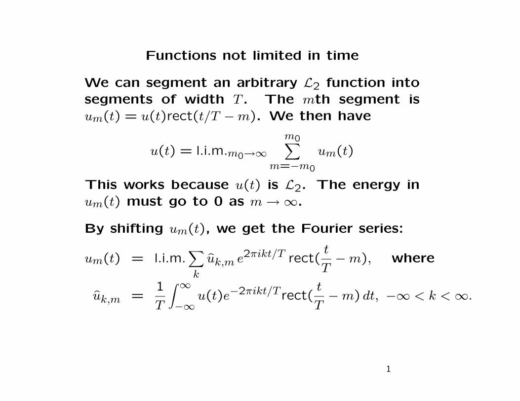
�

Functions not limited in time

We can segment an arbitrary L2 function into segments of width T . The mth segment is um(t) = u(t)rect(t/T − m). We then have

m0

u(t) = l.i.m.m0→∞ um(t) m=−m0

This works because u(t) is L2. The energy in um(t) must go to 0 as m → ∞.

By shifting um(t), we get the Fourier series: � t um(t) = l.i.m. uk,m e 2πikt/T rect(

T − m), where

k

ˆ =1 � ∞

u(t)e−2πikt/T rect(T

t − m) dt, −∞ < k < ∞.uk,m T −∞

1

�

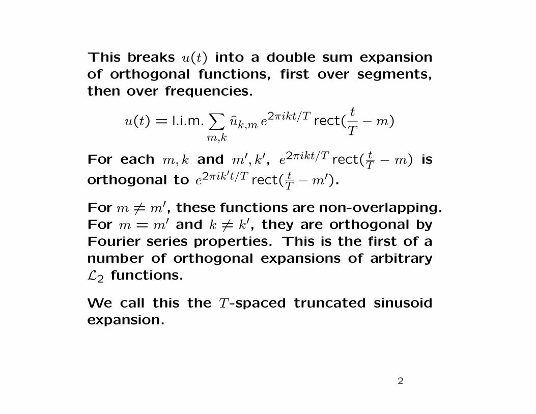
This breaks u(t) into a double sum expansion of orthogonal functions, first over segments, then over frequencies. � t

u(t) = l.i.m. uk,m e 2πikt/T rect(T

− m) m,k

For each m, k and m′, k′, e2πikt/T rect(Tt − m) is

orthogonal to e2πik′t/T rect(Tt − m′).

For m =� m′, these functions are non-overlapping. For m = m′ and k = k′, they are orthogonal by Fourier series properties. This is the first of a number of orthogonal expansions of arbitrary L2 functions.

We call this the T -spaced truncated sinusoid expansion.

2

� t u(t) = l.i.m. uk,m e 2πikt/T rect(

T − m)

m,k

This is the conceptual basis for algorithms such

as voice compression that segment the wave­

form and then process each segment.

It matches our intuition about frequency well;

that is, in music, notes (frequencies) keep chang­

ing.

The awkward thing is that the segmentation

parameter T is arbitrary and not fundamental.

3

� �

C Fourier transform: u(t) : R C to u(f ) : R→ →

u(f ) = ∞

u(t)e−2πift dt. −∞

2πift df. u(t) = ∞

u(f)e −∞

For “well-behaved functions,” first integral ex­

ists for all f, second exists for all t and results

in original u(t).

What does well-behaved mean? It means that

the above is true.

4

�

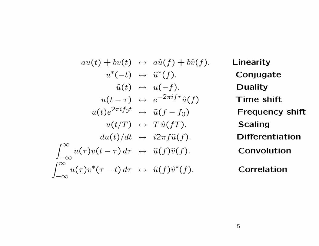
au(t) + bv(t)

u∗(−t)

u(t)

u(t − τ )

u(t)e 2πif0t

u(t/T )

du(t)/dt∞

u(τ )v(t − τ ) dτ � −∞∞

u(τ )v∗(τ − t) dτ −∞

au(f) + bv(f).↔

u∗(f).↔

↔ u(−f ).

e−2πifτ u(f )↔

↔ u(f − f0)

T u(fT ).↔

i2πfu(f ).↔

u(f)v(f ).↔

u(f)v∗(f).↔

Linearity

Conjugate

Duality

Time shift

Frequency shift

Scaling

Differentiation

Convolution

Correlation

5

� �

� �

� �

Two useful special cases of any Fourier trans­

form pair are:

u(0) = ∞

u(f) df ; −∞

u(0) = ∞

u(t) dt. −∞

Parseval’s theorem: ∞

u(t)v∗(t) dt = ∞

u(f)v∗(f) df. −∞ −∞

Replacing v(t) by u(t) yields the energy equa­

tion, ∞

u(t)|2 dt = ∞

u(f)|2 df. −∞

|−∞

|ˆ

6

� �

C Fourier transform: u(t) : R C to u(f ) : R→ →

u(f ) = ∞

u(t)e−2πift dt. −∞

u(t) = ∞

u(f)e 2πift df. −∞

If u(t) is L1, first integral exists for all f. Fur­

thermore u(f) must be a continuous function.

If u(f) is L1, second integral exists for all t and

u(t) is continuous.

Unfortunately, we don’t always get back to

same function that we started with.

7

Not enough functions are L1 to provide suit­

able models for communication systems.

For example, sinc(t) is not L1.

Also, functions with discontinuities cannot be

Fourier transforms of L1 functions.

Finally, L1 functions might have infinite energy.

L2 functions turn out to be the “right” class.

{u(t) : R → C} is �L2 if measurable and if

∞ 2 dt < ∞

−∞ |u(t)|

8

L2 functions and Fourier transforms

Theorem: If {u(t) : R C} is L2 and time lim­→ited, it is also L1.

Proof: |u(t)|2 ≤ |u(t)| + 1, so � B � B

A |u(t)| dt ≤

A |u(t)|2 dt + (B − A) < ∞. �

− −For any L2 function u(t) and A > 0, let vA(t) be u(t) truncated to [−A, A],

t vA(t) = u(t)rect( )

2A

Then vA(t) is both L2 and L1. Its Fourier trans­form vA(f) exists for all f and is continuous. � A

vA(f ) = u(t)e−2πift dt. −A

9

L2 functions and Fourier transforms

Recall that if {u(t) : R C} is L and time→ 2 limited, it is also L1.

Proof: |u(t)| ≤ |u(t)|2 + 1, so � B � B

A |u(t)| dt ≤

A |u(t)|2 dt + (B − A) < ∞. �

− −For any L2 function u(t) and A > 0, consider u(t)rect(2

tA). This function is time limited and

L2, so it is L1.

Its Fourier transform vA(f ) exists for all f and is continuous. � A

vA(f ) = u(t)e−2πift dt. −A

10

�

�

�

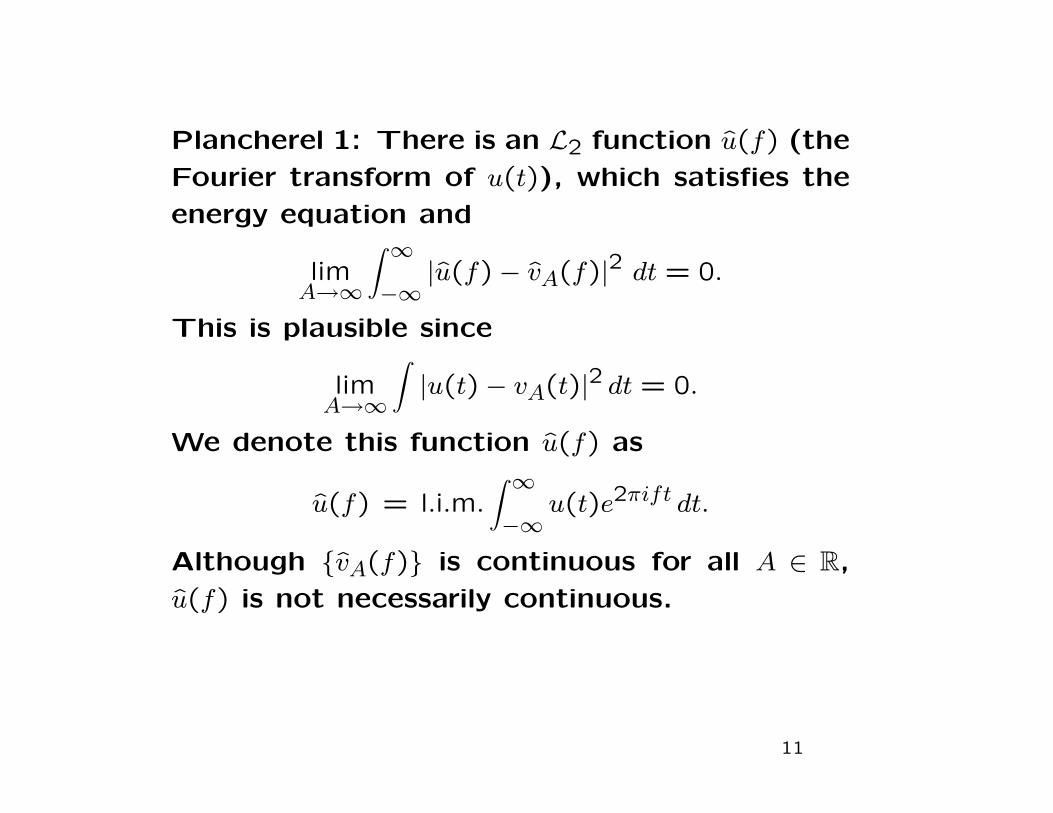
Plancherel 1: There is an L2 function u(f ) (the

Fourier transform of u(t)), which satisfies the

energy equation and ∞

2lim ˆ dt = 0.A→∞ −∞

|u(f) − vA(f)|

This is plausible since

lim |u(t) − vA(t) 2 dt = 0. A→∞

|

We denote this function u(f) as

u(f) = l.i.m. ∞

u(t)e 2πift dt. −∞

Although {vA(f )} is continuous for all A ∈ R,

u(f) is not necessarily continuous.

11

� �

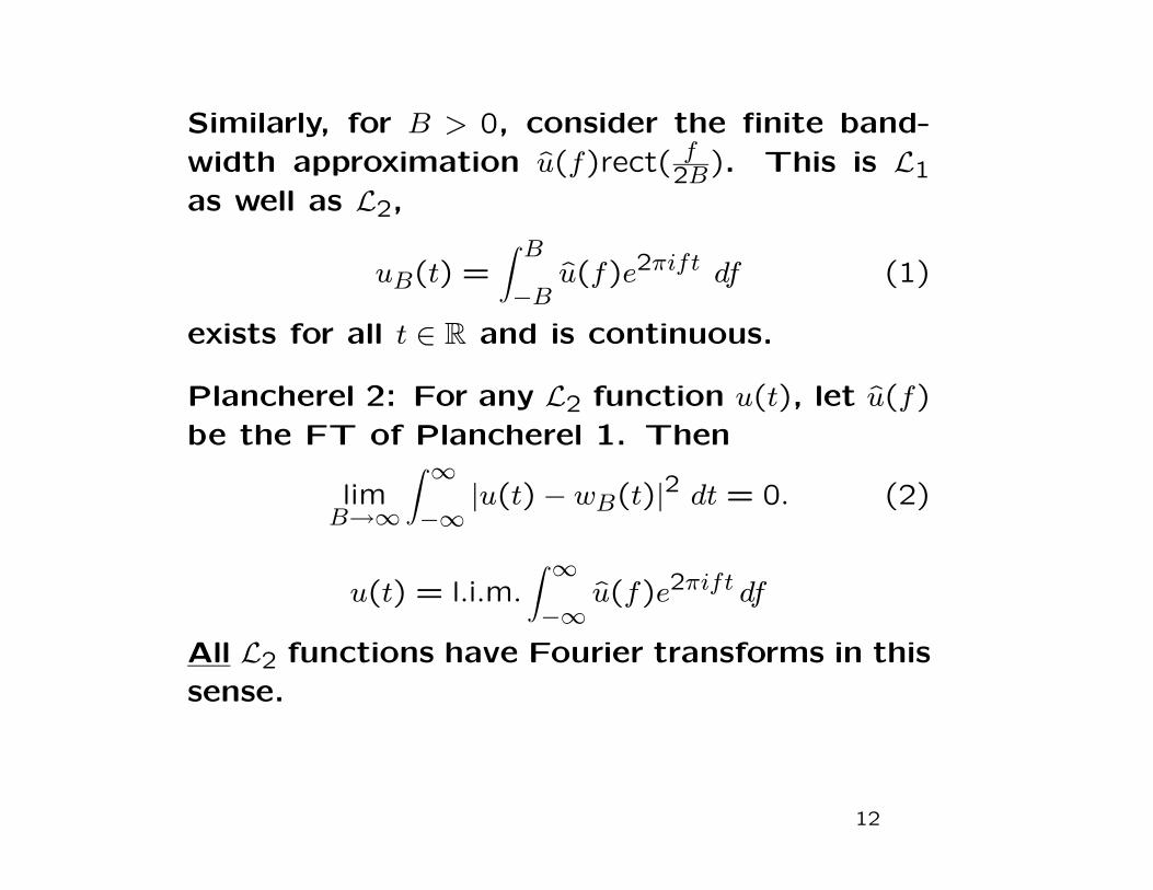
Similarly, for B > 0, consider the finite band­

width approximation u(f)rect( f ). This is L12B as well as L2, � B

uB(t) = u(f)e 2πift df (1) −B

exists for all t ∈ R and is continuous.

Plancherel 2: For any L2 function u(t), let u(f)

be the FT of Plancherel 1. Then

lim ∞

u(t) − wB(t)|2 dt = 0. (2) B→∞ −∞

|

2πift dfu(t) = l.i.m. ∞

u(f)e −∞

All L2 functions have Fourier transforms in this

sense.

12

L2 waveforms do not include some favorite waveforms of most EE’s.

Constants, sine waves, impulses are all infinite energy “functions.”

Constants and sine waves result from refusing to explicitly model when “very long-lasting” functions terminate. Impulses result from re­fusing to model how long very short pulses last. Both models ignore energy.

These are useful models for many problems.

As communication waveforms, infinite energy waveforms make MSE quantization results mean­ingless. Also they make most channel results meaningless.

13

������� ������

� � �

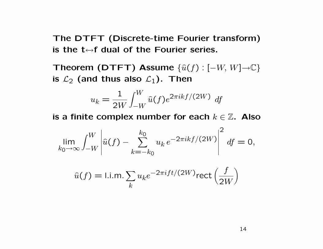
The DTFT (Discrete-time Fourier transform)

is the t f dual of the Fourier series. ↔

Theorem (DTFT) Assume {u(f ) : [−W, W ] C}→is L2 (and thus also L1). Then

uk =1 � W

u(f )e 2πikf/(2W ) df 2W −W

is a finite complex number for each k ∈ Z. Also

k02� W

uk e−2πikf/(2W )lim

k0→∞ −Wu(f ) − df = 0,

k=−k0

fuke−2πift/(2W )u(f ) = l.i.m. rect

2Wk

14

� �

�

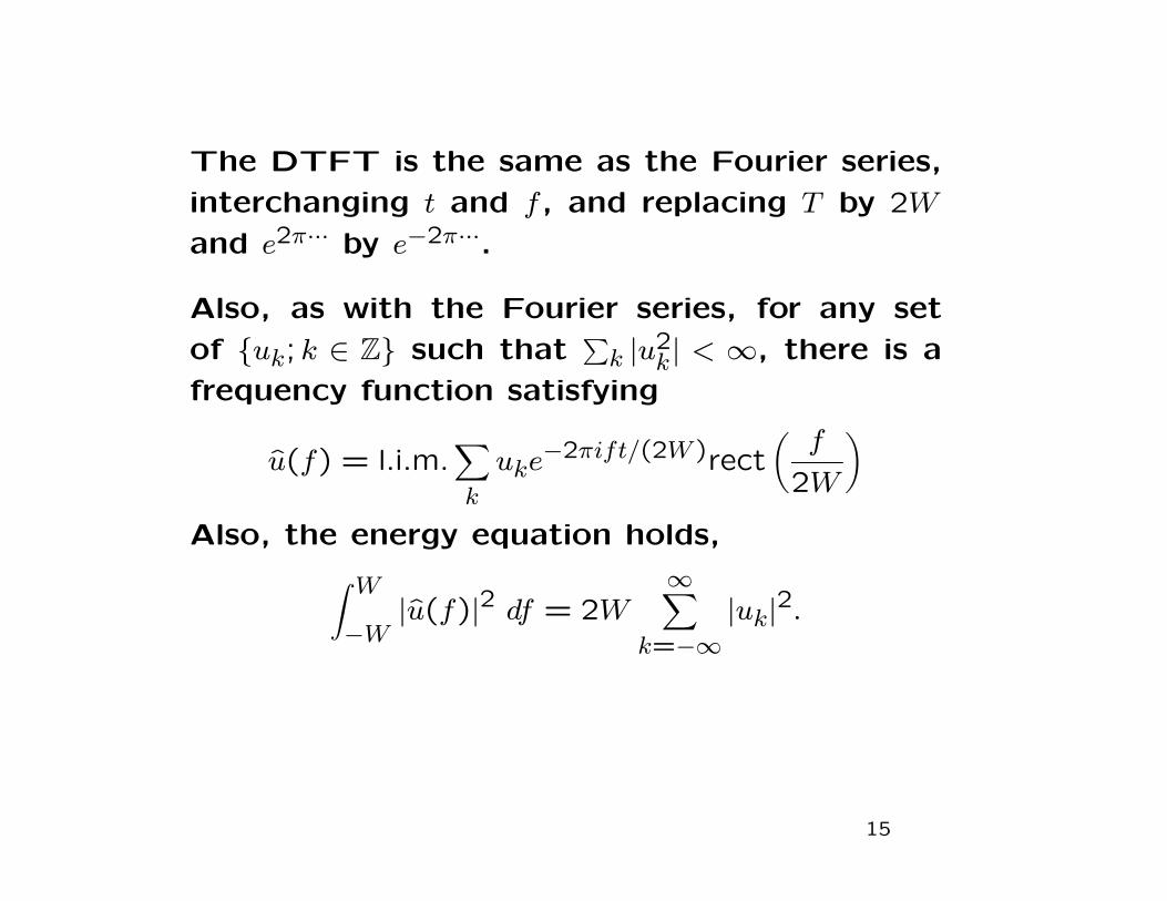
The DTFT is the same as the Fourier series,

interchanging t and f , and replacing T by 2W

and e 2π by e −2π··· ···.

Also, as with the Fourier series, for any set

of {uk ; k ∈ Z} such that �

k |u 2 k | < ∞, there is a

frequency function satisfying � f u(f ) = l. i. m. uke −2πift/ (2W )rect

2Wk

Also, the energy equation holds, � −

W

W |u(f )| 2 df = 2W

∞|uk |2 .

k =−∞

15

� �

�

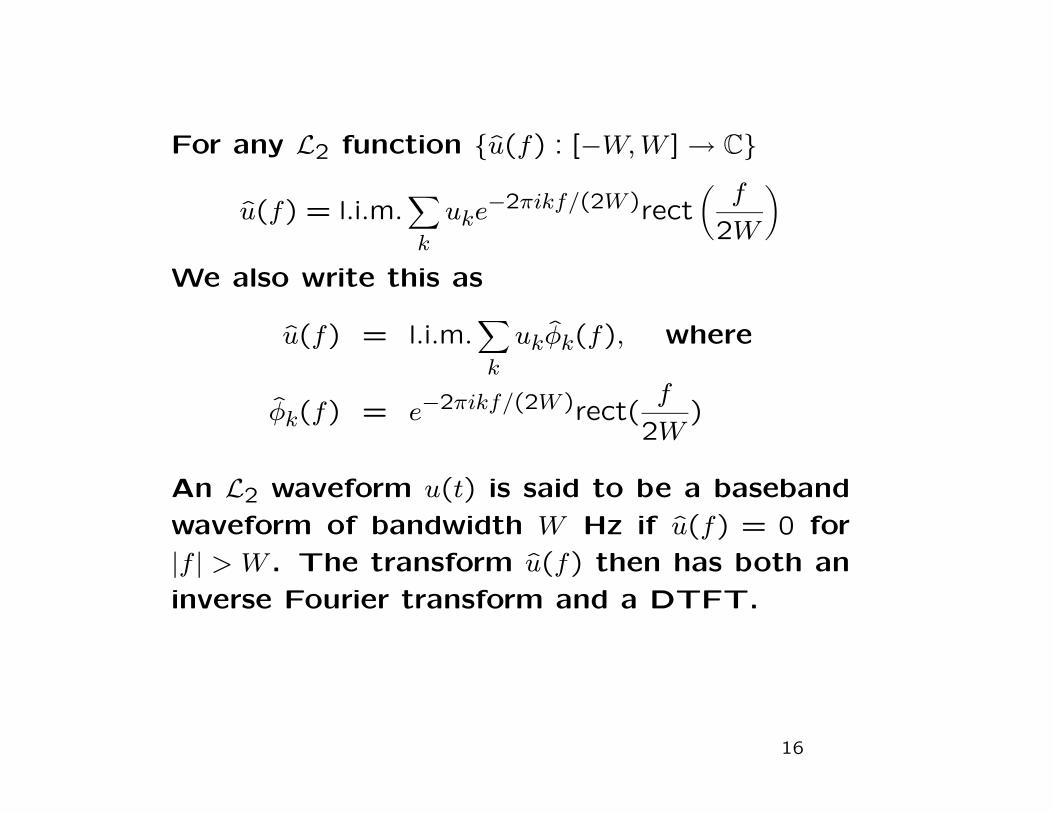
For any L2 function {u(f) : [−W, W ] C}→

u(f) = l.i.m. �

uke−2πikf/(2W )rect f

2Wk

We also write this as

u(f) = l.i.m. ukφk(f), where k

φk(f) = e−2πikf/(2W )rect( f

)2W

An L2 waveform u(t) is said to be a baseband

waveform of bandwidth W Hz if u(f) = 0 for

|f | > W . The transform u(f) then has both an

inverse Fourier transform and a DTFT.

16

� �

� �

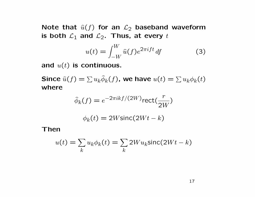
Note that u(f) for an L2 baseband waveform

is both L1 and L2. Thus, at every t � W u(t) = u(f)e 2πift df (3)

−W

and u(t) is continuous.

φk(f) = e−2πikf/(2W )rect(

Since u(f) = ukφk(f), we have u(t) = ukφk(t) where

r )

2W

φk(t) = 2W sinc(2Wt − k)

Then

u(t) = ukφk(t) = 2Wuksinc(2Wt − k) k k

17

�

�

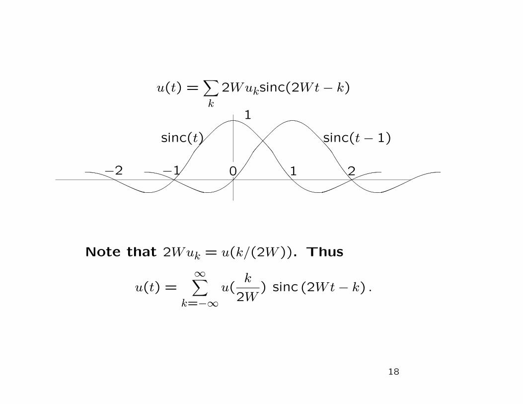
u(t) = 2Wuksinc(2Wt − k) k

1

sinc(t) sinc(t − 1)

−2 −1 0 1 2

Note that 2Wuk = u(k/(2W )). Thus

∞ k u(t) = u( ) sinc (2Wt − k) .

2Wk=−∞

18

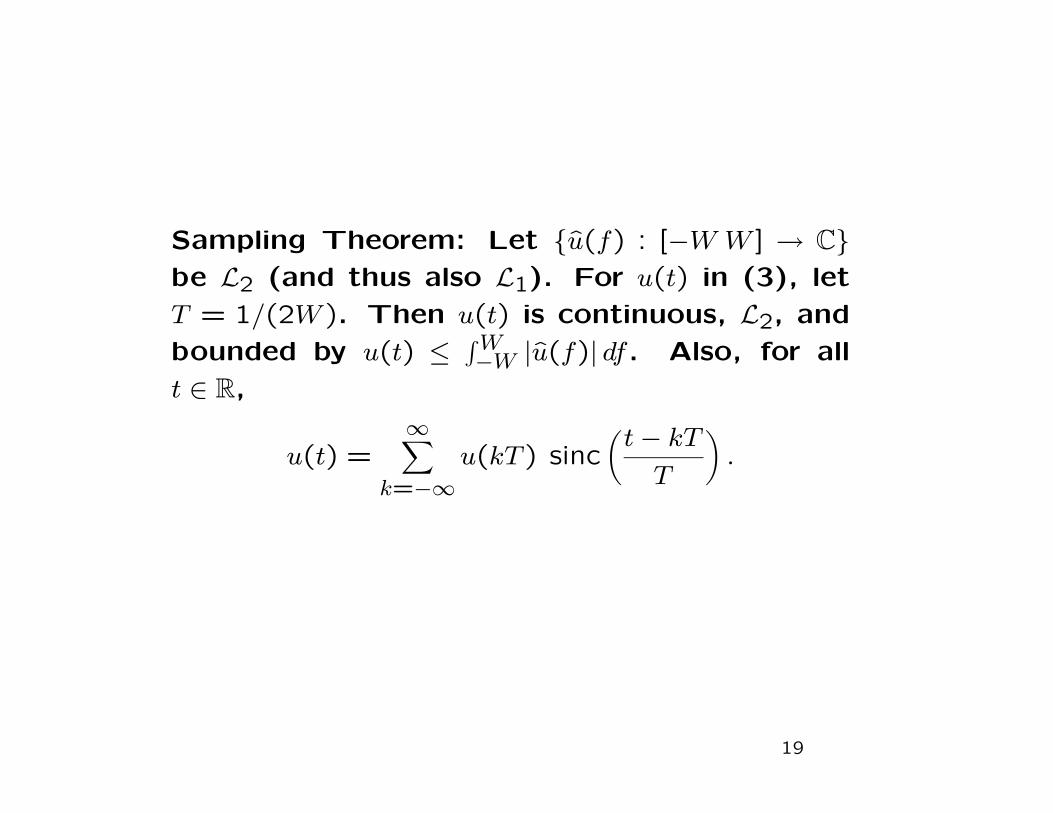
Sampling Theorem: Let {u(f) : [−W W ] C}→

be L2 (and thus also L1). For u(t) in (3), let

T = 1/(2W ). Then u(t) is continuous, L2, and

bounded by u(t) ≤ � −WW |u(f)| df. Also, for all

t ∈ R,

∞ � � u(t) =

� u(kT ) sinc

t − kT .

Tk=−∞

19

Note that we started with {u(f ) : [−W, W ] C}.→

There are other bandlimited functions, limited

to [−W, W ], which are not continuous. That

is, there are functions that are L2 equivalent

to the u(t) above. They have the same FT,

but they are different on any arbitrary set of

points of measure 0.

The sampliing theorem does not hold for these

functions.

Baseband limited to W , from now on, means

the continuous function whose Fourier trans­

form is limited to [−W, W ].

20

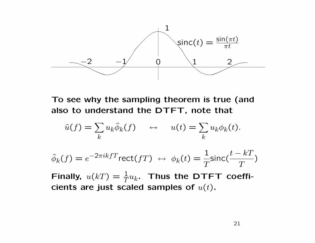
1

sinc(t) = sin(πtπt)

0 1 2−2 −1

To see why the sampling theorem is true (and

also to understand the DTFT, note that

u(f) = � k

uk φk(f) ↔ u(t) = � k

ukφk(t).

φk(f) = e−2πikfT rect(fT ) ↔ φk(t) = 1

T sinc(

t − kT

T )

Finally, u(kT ) = T 1 uk. Thus the DTFT coeffi­

cients are just scaled samples of u(t).

21

MIT OpenCourseWare http://ocw.mit.edu

6.450 Principles of Digital Communication I Fall 2009

For information about citing these materials or our Terms of Use, visit: http://ocw.mit.edu/terms.