ECE 1100 Introduction to Electrical and Computer Engineeringcourses.egr.uh.edu/ECE/ECE6341/Class...
54
Prof. David R. Jackson ECE Dept. Spring 2016 Notes 6 ECE 6341 1
Transcript of ECE 1100 Introduction to Electrical and Computer Engineeringcourses.egr.uh.edu/ECE/ECE6341/Class...

Prof. David R. Jackson ECE Dept.
Spring 2016
Notes 6
ECE 6341
1
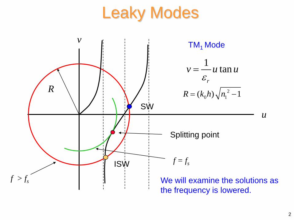
Leaky Modes
2
f = fs
v
u
TM1 Mode
ISW
SW
f > fs We will examine the solutions as the frequency is lowered.
Splitting point
1 tanr
v u uε
=
R 20 1( ) 1R k h n= −
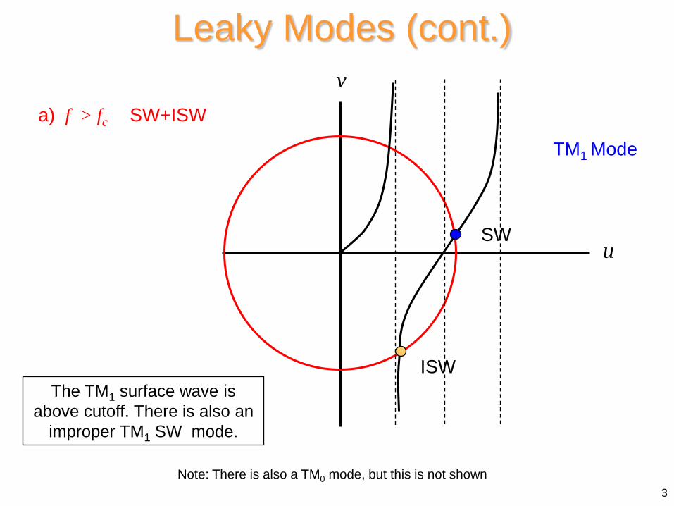
Leaky Modes (cont.)
a) f > fc SW+ISW
v
u
ISW
SW
3
TM1 Mode
The TM1 surface wave is above cutoff. There is also an
improper TM1 SW mode.
Note: There is also a TM0 mode, but this is not shown
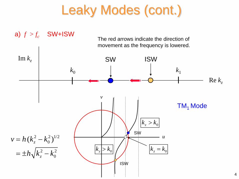
Leaky Modes (cont.) a) f > fc SW+ISW
Im kz
k1
SW
Re kz k0
ISW
The red arrows indicate the direction of movement as the frequency is lowered.
2 2 1/20
2 20
( )z
z
v h k k
h k k
= −
= ± −
4
0zk k>
0zk k> 0zk k=
v
u
ISW
SW
TM1 Mode
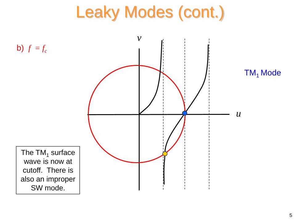
b) f = fc
Leaky Modes (cont.) v
u
5
TM1 Mode
The TM1 surface wave is now at cutoff. There is
also an improper SW mode.
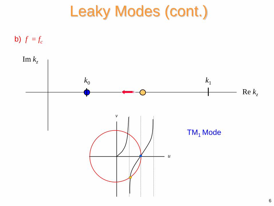
b) f = fc
Leaky Modes (cont.)
6
Im kz
k1
Re kz k0
v
u
TM1 Mode
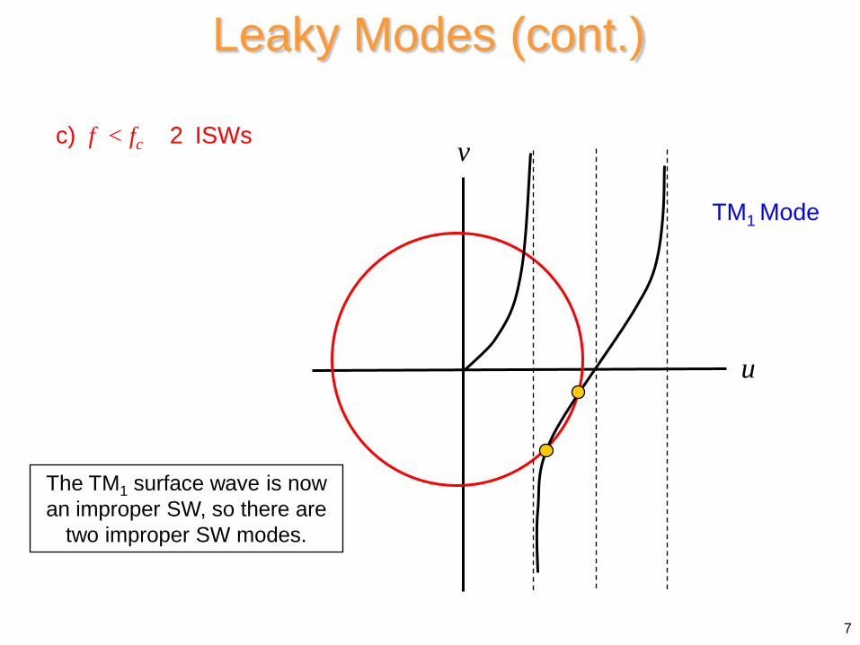
c) f < fc 2 ISWs
Leaky Modes (cont.)
v
u
7
The TM1 surface wave is now an improper SW, so there are
two improper SW modes.
TM1 Mode
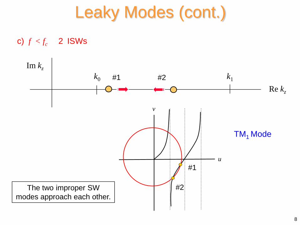
c) f < fc 2 ISWs
Im kz k1
Re kz k0
Leaky Modes (cont.)
8
The two improper SW modes approach each other.
v
u
TM1 Mode
#1 #2
#1
#2
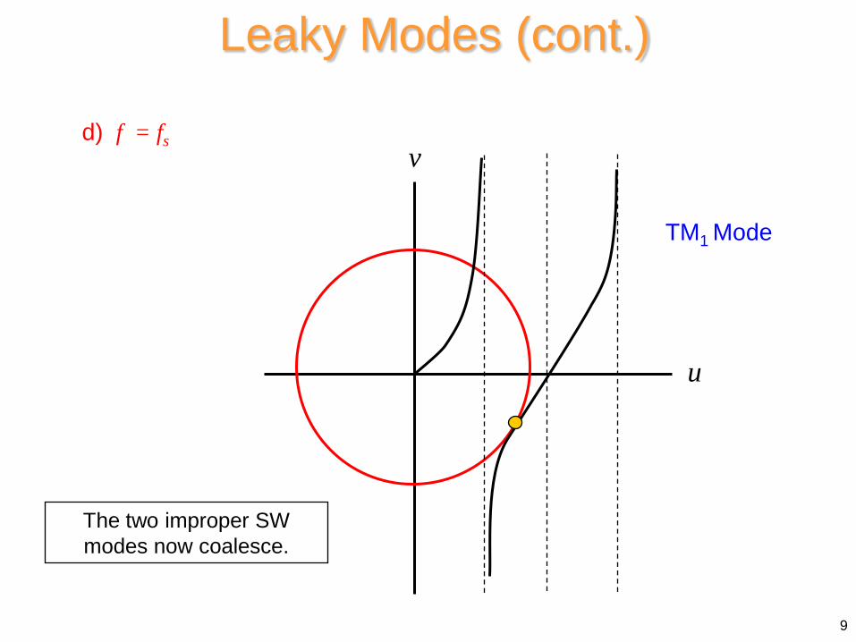
d) f = fs
Leaky Modes (cont.)
v
u
9
The two improper SW modes now coalesce.
TM1 Mode
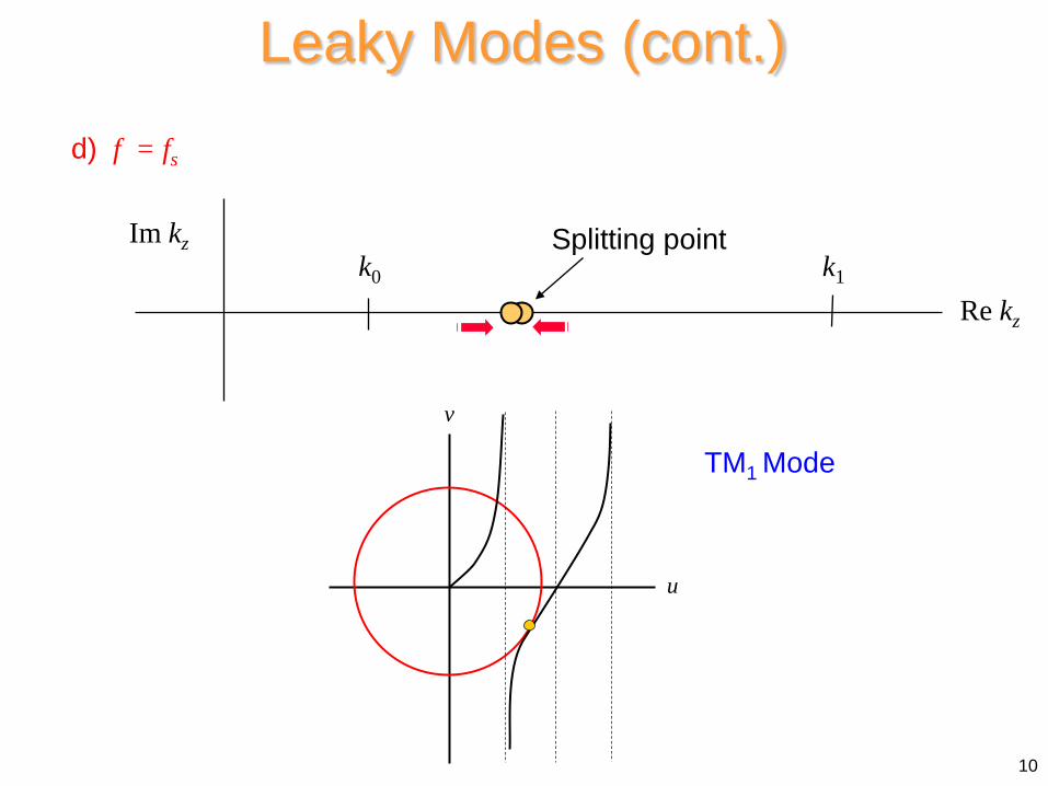
d) f = fs
Leaky Modes (cont.)
10
Im kz k1
Re kz k0
Splitting point
v
u
TM1 Mode
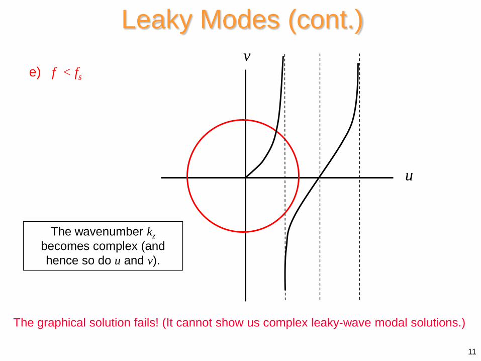
e) f < fs
Leaky Modes (cont.) v
u
The graphical solution fails! (It cannot show us complex leaky-wave modal solutions.)
11
The wavenumber kz becomes complex (and hence so do u and v).
Leaky Modes (cont.)
12
Im kz
k1
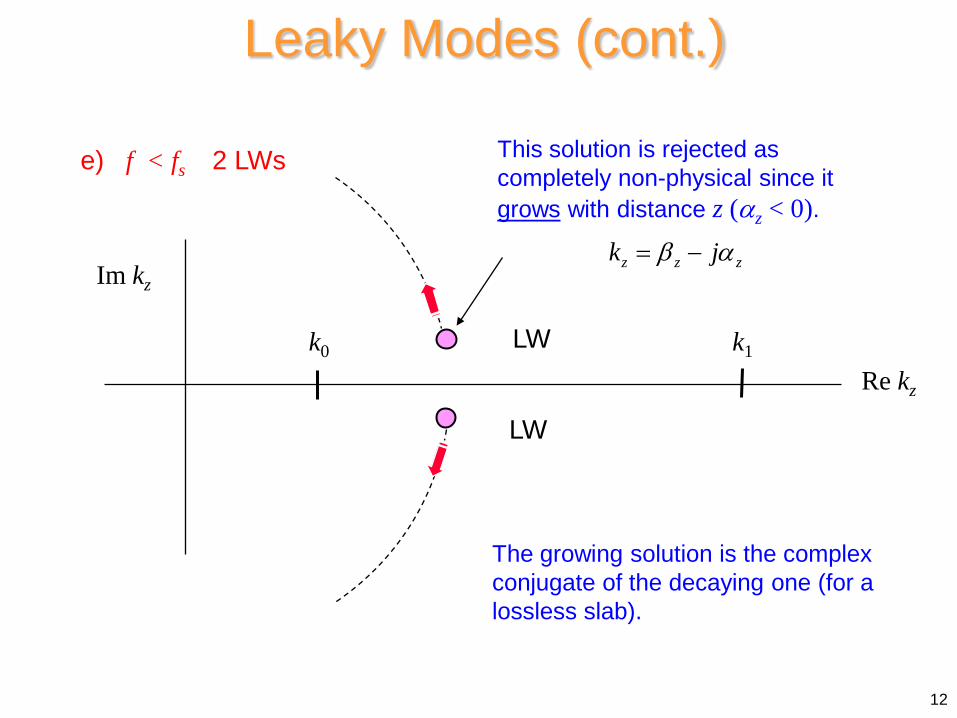
e) f < fs 2 LWs
Re kz k0
LW
LW
This solution is rejected as completely non-physical since it grows with distance z (αz < 0).
The growing solution is the complex conjugate of the decaying one (for a lossless slab).
z z zk jβ α= −
Leaky Modes (cont.)
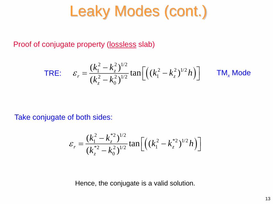
Proof of conjugate property (lossless slab)
Take conjugate of both sides:
( )2 2 1/2
2 2 1/2112 2 1/2
0
( ) tan ( )( )
zr z
z
k k k k hk k
ε − = − −
( )2 *2 1/2
2 *2 1/211*2 2 1/2
0
( ) tan ( )( )
zr z
z
k k k k hk k
ε − = − −
Hence, the conjugate is a valid solution.
TRE:
13
TMx Mode
Leaky Modes (cont.)
a) f > fc
14
Im kz
k1
SW
Re kz
k0
ISW
b) f = fc
Im kzk1
Re kz
k0c) f < fc
Im kzk1
Re kz
k0
splitting point
d) f = fs
Im kz
k1
Re kz
k0
LW
LWe) f < fs
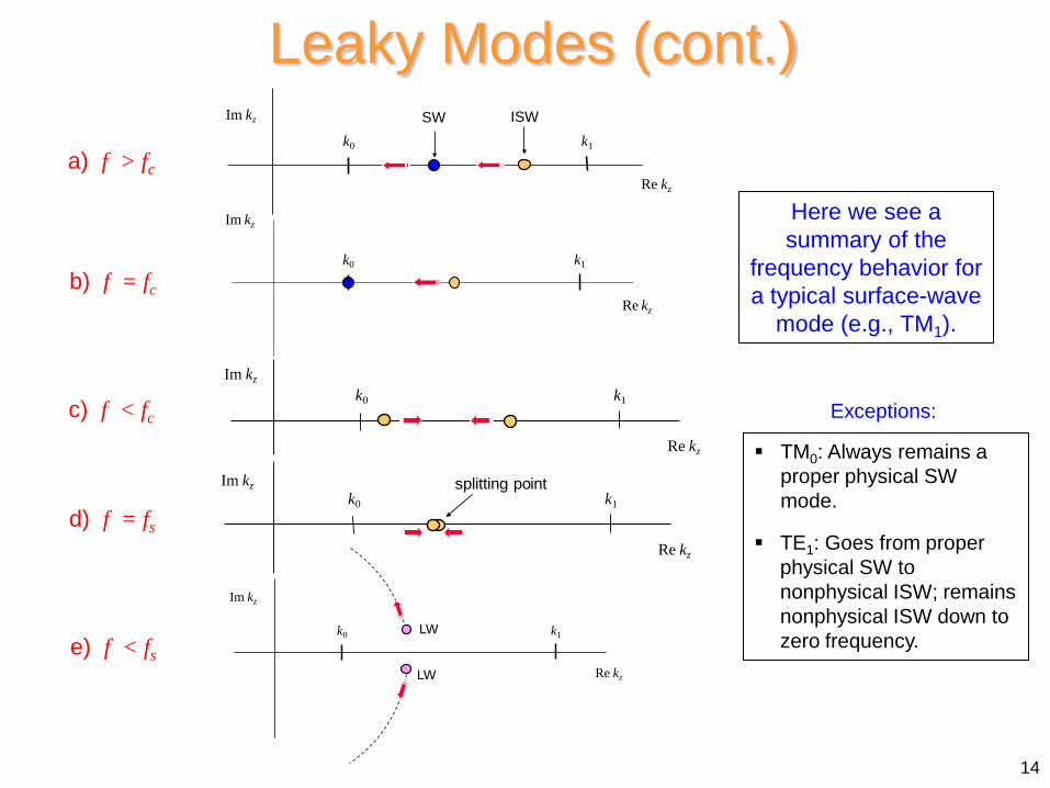
Here we see a summary of the
frequency behavior for a typical surface-wave
mode (e.g., TM1).
TM0: Always remains a proper physical SW mode.
TE1: Goes from proper physical SW to nonphysical ISW; remains nonphysical ISW down to zero frequency.
Exceptions:
Im kz
k1
Re kz
k0
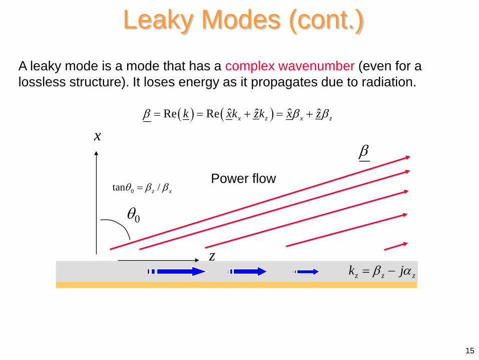
Leaky Modes (cont.) A leaky mode is a mode that has a complex wavenumber (even for a lossless structure). It loses energy as it propagates due to radiation.
15
z
Power flow
βx
z z zk jβ α= −
( ) ( )ˆ ˆˆ ˆRe Re x z x zk xk zk x zβ β β= = + = +
θ0
0tan /z xθ β β=
Leaky Modes (cont.)
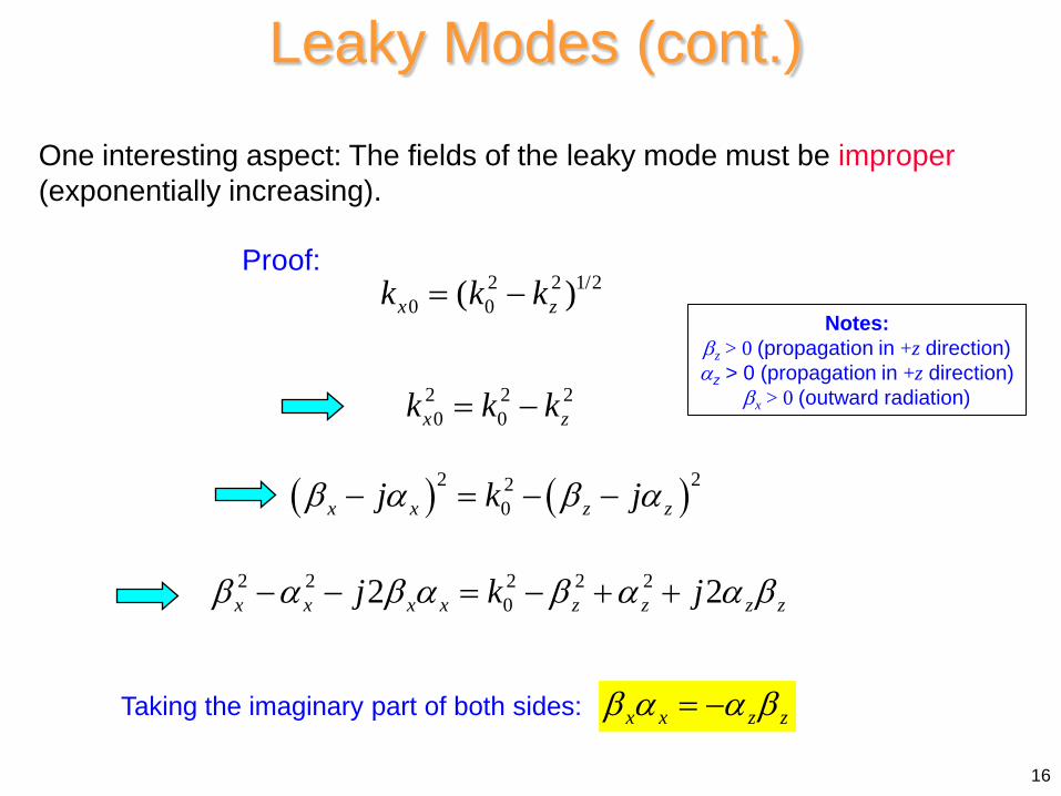
One interesting aspect: The fields of the leaky mode must be improper (exponentially increasing).
Proof: 2 2 1/2
0 0( )x zk k k= −
2 2 20 0x zk k k= −
( ) ( )2 220x x z zj k jβ α β α− = − −
2 2 2 2 202 2x x x x z z z zj k jβ α β α β α α β− − = − + +
x x z zβ α α β= −Taking the imaginary part of both sides:
16
Notes: βz > 0 (propagation in +z direction) αz > 0 (propagation in +z direction)
βx > 0 (outward radiation)
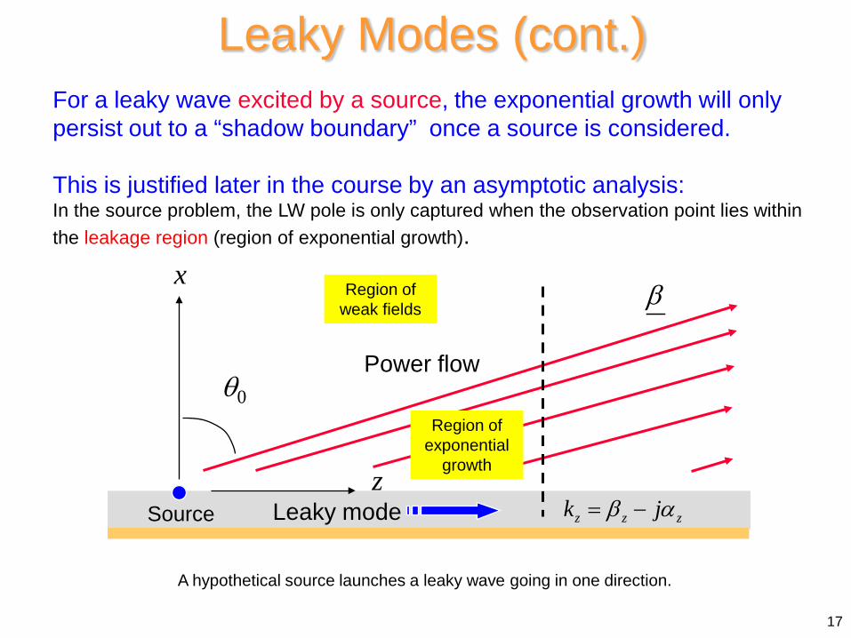
Leaky Modes (cont.) For a leaky wave excited by a source, the exponential growth will only persist out to a “shadow boundary” once a source is considered. This is justified later in the course by an asymptotic analysis: In the source problem, the LW pole is only captured when the observation point lies within the leakage region (region of exponential growth).
17
θ0
z
Power flow
Leaky mode
βx
Region of exponential
growth
Region of weak fields
z z zk jβ α= −Source
A hypothetical source launches a leaky wave going in one direction.
A requirement for a leaky mode to be strongly physical is that the wavenumber must lie within the “physical region” where is wave is a fast wave* (βz = Re kz < k0).
Leaky Modes (cont.)
A leaky-mode is considered to be “physical” if we can measure a significant contribution from it along the interface (θ0 = 90o) .
Basic reason: The LW pole is not captured in the complex plane in the source problem if the LW is a slow wave.
18 * This is justified by asymptotic analysis, given later.
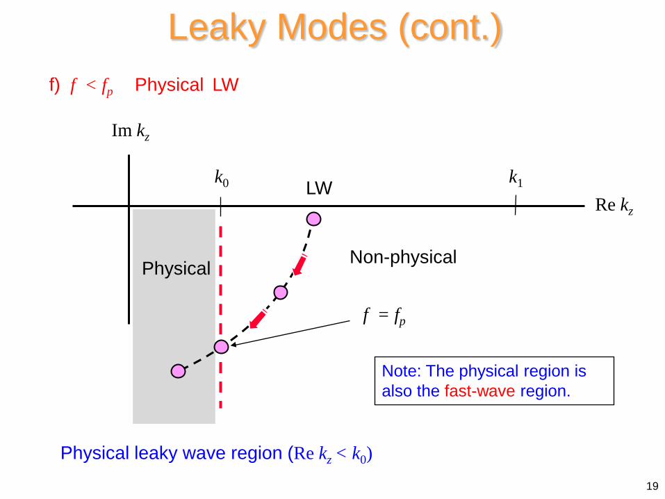
f) f < fp Physical LW
Physical leaky wave region (Re kz < k0)
Leaky Modes (cont.)
19
Im kz
k1
Re kz k0 LW
f = fp
Physical Non-physical
Note: The physical region is also the fast-wave region.
If the leaky mode is within the physical (fast-wave) region, a wedge-shaped radiation region will exist.
Leaky Modes (cont.)
This is illustrated on the next two slides.
20
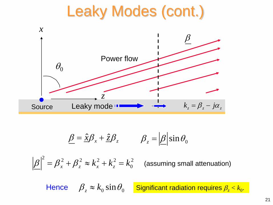
0sinzβ β θ=
2 2 2 2 2 20x z x zk k kβ β β= + ≈ + =
0 0sinz kβ θ≈Hence
Leaky Modes (cont.)
(assuming small attenuation)
ˆ ˆx zx zβ β β= +
Significant radiation requires βz < k0. 21
θ0
z
Power flow
Leaky mode
x
z z zk jβ α= −Source
β
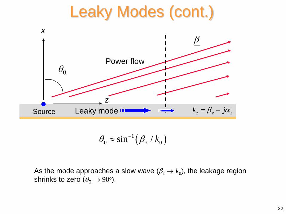
( )10 0sin /z kθ β−≈
Leaky Modes (cont.)
22
θ0
z
Power flow
Leaky mode
x
z z zk jβ α= −Source
β
As the mode approaches a slow wave (βz → k0), the leakage region shrinks to zero (θ0 → 90o).
Leaky Modes (cont.)
0nj
nI I e φ+=
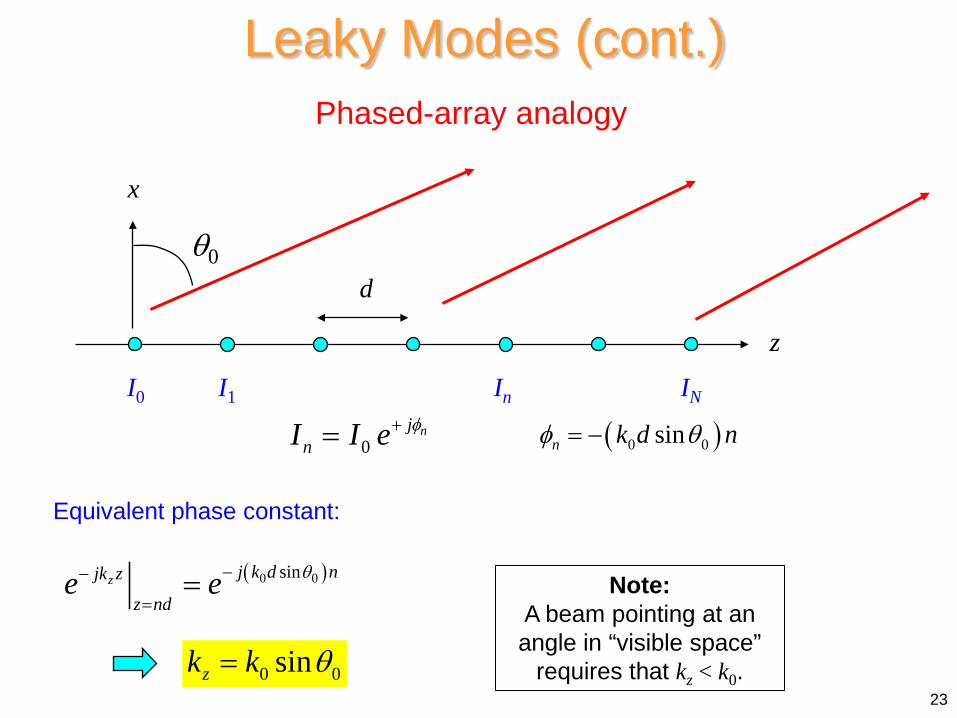
Phased-array analogy
z
I0
x
I1 In IN
d θ0
0 0sinzk k θ=23
Note: A beam pointing at an angle in “visible space”
requires that kz < k0.
( )0 0sinz j k d njk z
z nde e θ−−
==
( )0 0sinn k d nφ θ= −
Equivalent phase constant:
Leaky Modes (cont.)
24
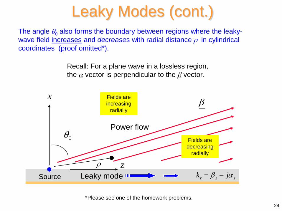
The angle θ0 also forms the boundary between regions where the leaky-wave field increases and decreases with radial distance ρ in cylindrical coordinates (proof omitted*).
θ0
z
Power flow
Leaky mode
x
Fields are decreasing
radially
z z zk jβ α= −Source
βFields are increasing
radially
ρ
*Please see one of the homework problems.
Recall: For a plane wave in a lossless region, the α vector is perpendicular to the β vector.
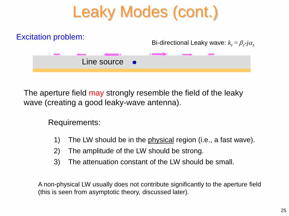
The aperture field may strongly resemble the field of the leaky wave (creating a good leaky-wave antenna).
Leaky Modes (cont.)
Requirements:
1) The LW should be in the physical region (i.e., a fast wave). 2) The amplitude of the LW should be strong. 3) The attenuation constant of the LW should be small.
A non-physical LW usually does not contribute significantly to the aperture field (this is seen from asymptotic theory, discussed later).
Excitation problem:
25
Line source
Bi-directional Leaky wave: kz = βz-jαz
Leaky Modes (cont.)
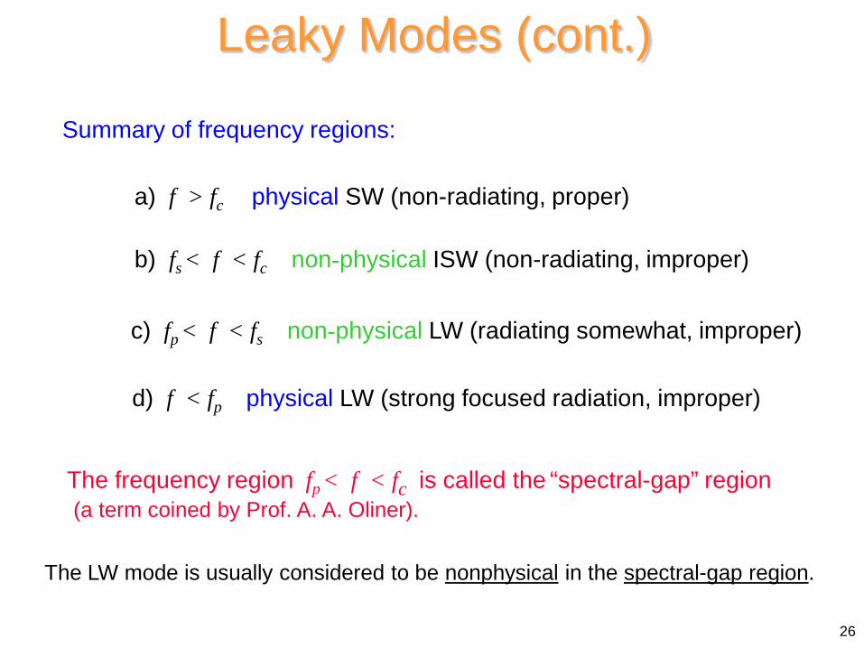
Summary of frequency regions:
a) f > fc physical SW (non-radiating, proper)
b) fs < f < fc non-physical ISW (non-radiating, improper)
c) fp < f < fs non-physical LW (radiating somewhat, improper)
d) f < fp physical LW (strong focused radiation, improper)
The frequency region fp < f < fc is called the “spectral-gap” region (a term coined by Prof. A. A. Oliner).
The LW mode is usually considered to be nonphysical in the spectral-gap region.
26
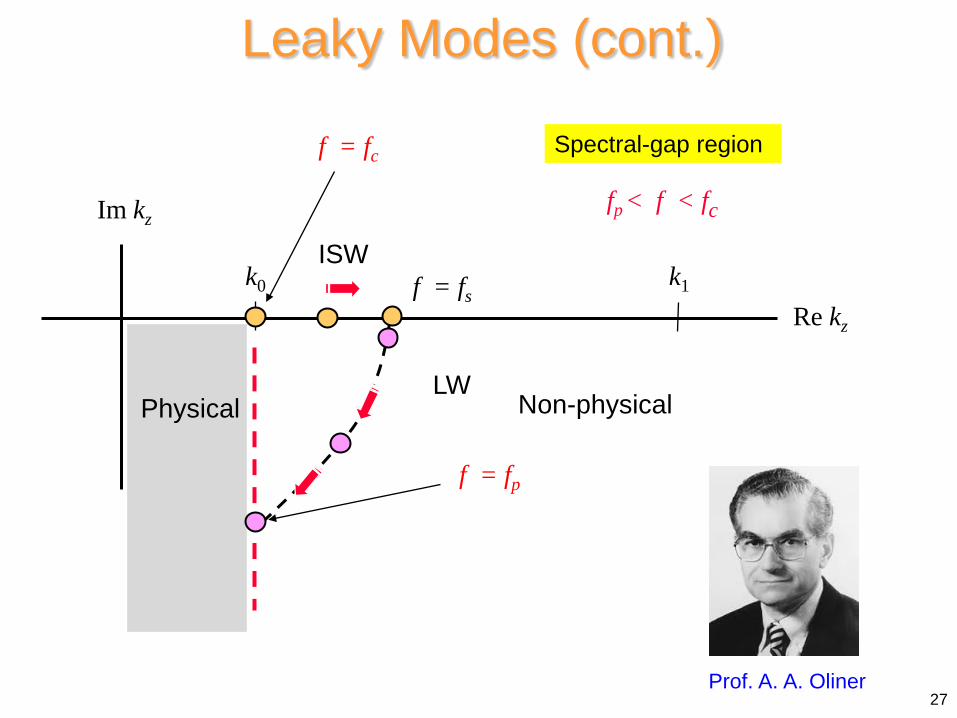
Leaky Modes (cont.)
27
Im kz
k1
Re kz k0
LW
f = fp
Physical Non-physical
ISW
f = fc
f = fs
Spectral-gap region
fp < f < fc
Prof. A. A. Oliner
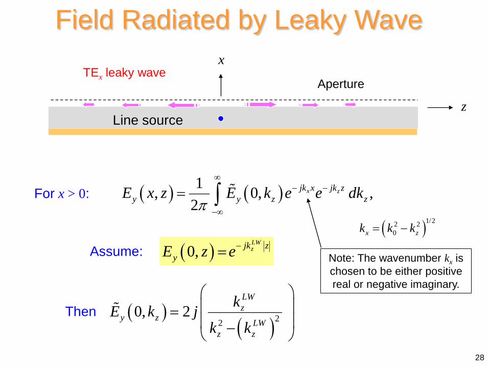
Field Radiated by Leaky Wave
( ) ( )1, 0, ,2
x zjk x jk zy y z zE x z E k e e dk
π
∞− −
−∞
= ∫
( )0,LWzjk z
yE z e−=
( )( )22
0, 2LWz
y z LWz z
kE k jk k
= −
28
For x > 0:
Then
Line source z
x
Aperture
( )1/22 20x zk k k= −
Note: The wavenumber kx is chosen to be either positive real or negative imaginary.
Assume:
TEx leaky wave
z / λ0
x / λ0
-10 10 0
0
10
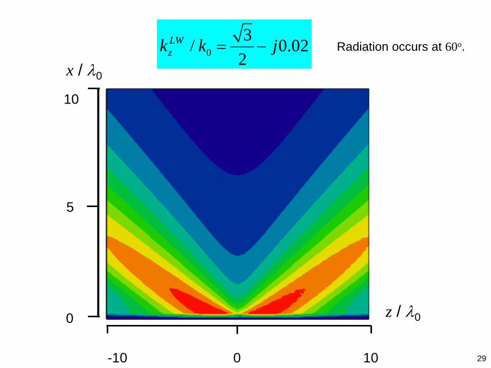
03/ 0.02
2LWzk k j= −
5
x / λ0
0
10
5
-10 0 10 29
Radiation occurs at 60o.
z / λ0
x / λ0
-10 10 0
0
10
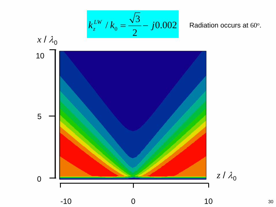
03/ 0.002
2LWzk k j= −
5
x / λ0
0
10
5
-10 0 10 30
Radiation occurs at 60o.
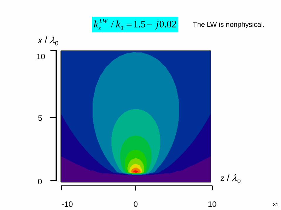
z / λ0
x / λ0
-10 10 0
0
10
0/ 1.5 0.02LWzk k j= −
5
x / λ0
0
10
5
-10 0 10 31
The LW is nonphysical.
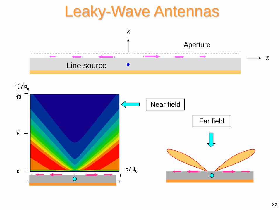
x / λ0
Leaky-Wave Antennas
Near field
Far field
32
Line source z
x
Aperture
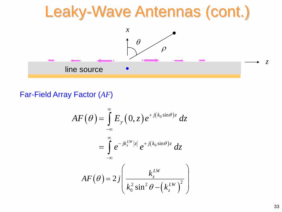
Leaky-Wave Antennas (cont.)
Far-Field Array Factor (AF)
( ) ( ) ( )
( )
0
0
sin
sin
0,
LWz
j k zy
j k zjk z
AF E z e dz
e e dz
θ
θ
θ∞
+
−∞
∞+−
−∞
=
=
∫
∫
( )( )22 2
0
2sin
LWz
LWz
kAF jk k
θθ
= −
33
x / λ0
line source z
x θ
ρ
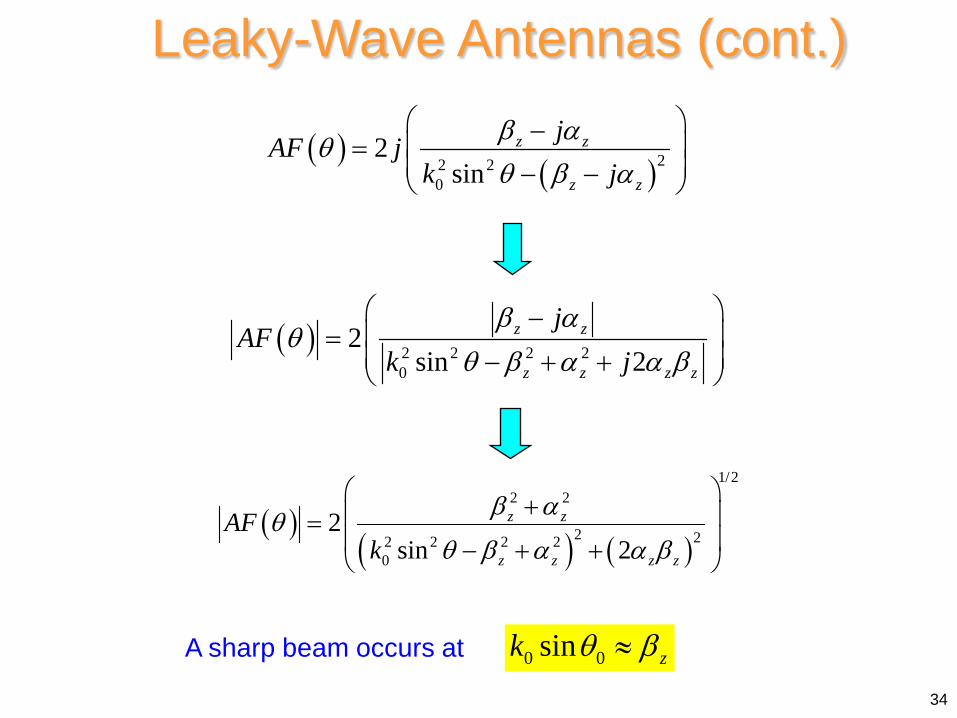
Leaky-Wave Antennas (cont.)
( )( )22 2
0
2sin
z z
z z
jAF jk j
β αθθ β α
− = − −
( ) 2 2 2 20
2sin 2
z z
z z z z
jAF
k jβ α
θθ β α α β
− = − + +
( )( ) ( )
1/22 2
2 22 2 2 20
2sin 2
z z
z z z z
AFk
β αθθ β α α β
+ = − + +
A sharp beam occurs at 0 0sin zk θ β≈
34
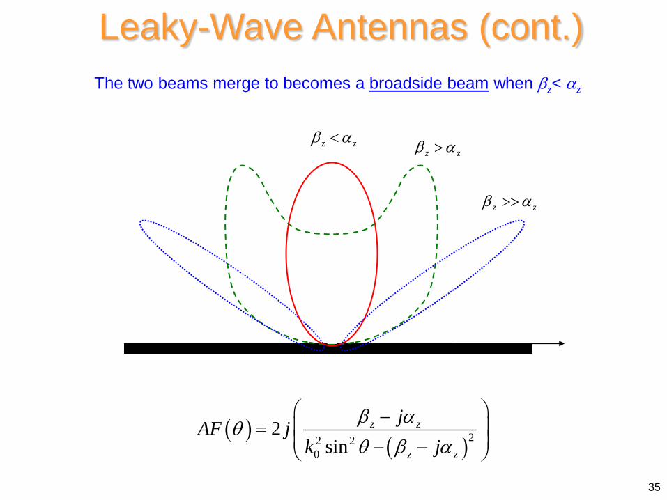
Leaky-Wave Antennas (cont.)
35
z zβ α<z zβ α>
z zβ α>>
z
( )( )22 2
0
2sin
z z
z z
jAF jk j
β αθθ β α
− = − −
The two beams merge to becomes a broadside beam when βz< αz
x / λ0
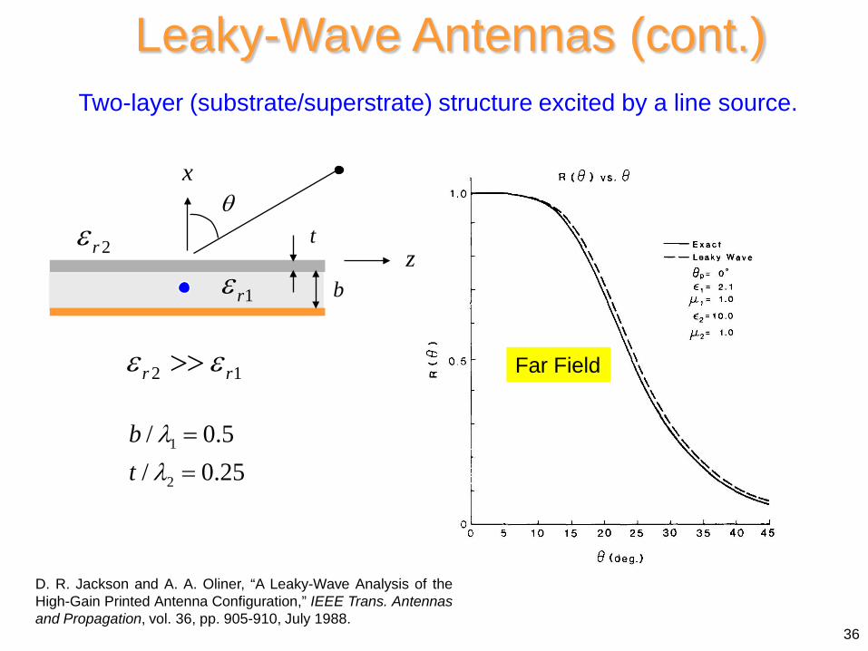
Leaky-Wave Antennas (cont.) Two-layer (substrate/superstrate) structure excited by a line source.
36
2 1r rε ε>>
1
2
/ 0.5/ 0.25
bt
λλ
==
1rε2rε
b
t
x θ
z
Far Field
D. R. Jackson and A. A. Oliner, “A Leaky-Wave Analysis of the High-Gain Printed Antenna Configuration,” IEEE Trans. Antennas and Propagation, vol. 36, pp. 905-910, July 1988.
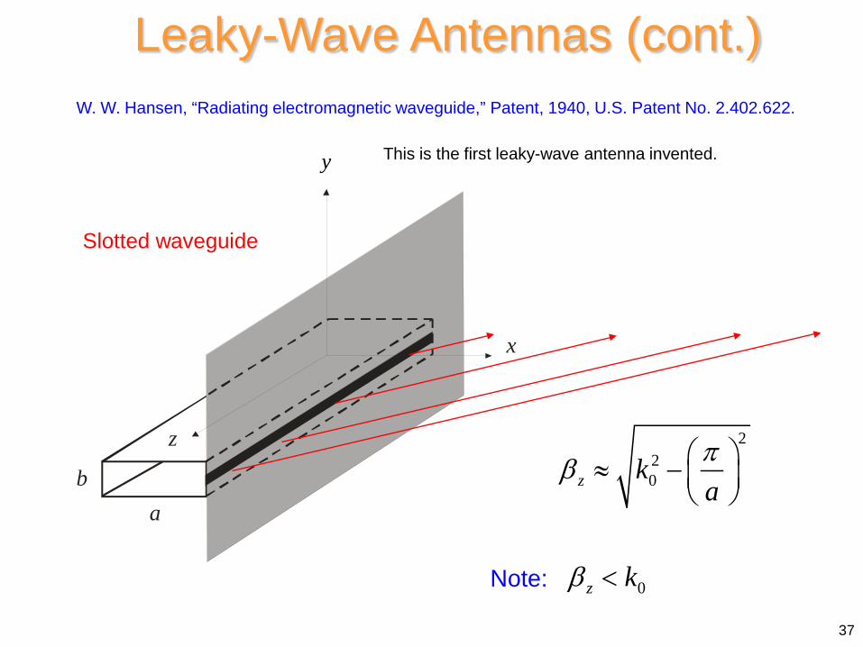
W. W. Hansen, “Radiating electromagnetic waveguide,” Patent, 1940, U.S. Patent No. 2.402.622.
ab
x
z
y
220z k
aπβ ≈ −
0z kβ <Note:
37
•W. W. Hansen, “Radiating electromagnetic waveguide,” Patent, 1940, U.S. Patent No. 2.402.622.
y This is the first leaky-wave antenna invented.
Slotted waveguide
Leaky-Wave Antennas (cont.)
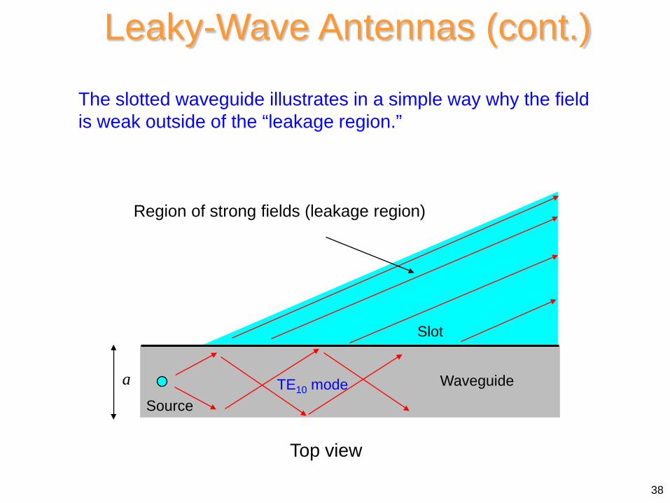
x / λ0 The slotted waveguide illustrates in a simple way why the field is weak outside of the “leakage region.”
38
Top view
Source
Slot
Region of strong fields (leakage region)
Waveguide a TE10 mode
Leaky-Wave Antennas (cont.)
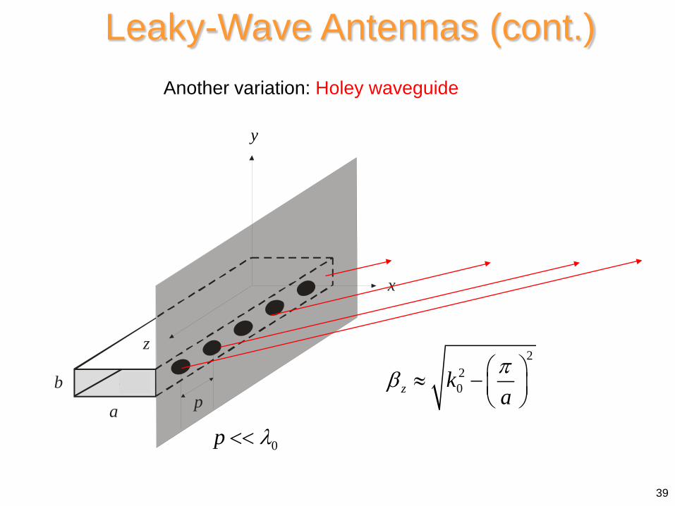
Another variation: Holey waveguide
220z k
aπβ ≈ −
39
0p λ<<a p
b
x
z
y
ε r
y
Leaky-Wave Antennas (cont.)
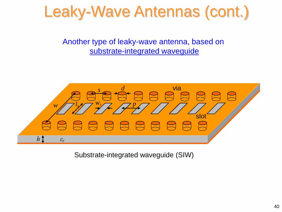
x / λ0 Another type of leaky-wave antenna, based on substrate-integrated waveguide
h εr
via d s
p ls ws w slot
40
Leaky-Wave Antennas (cont.)
Substrate-integrated waveguide (SIW)
x / λ0
41
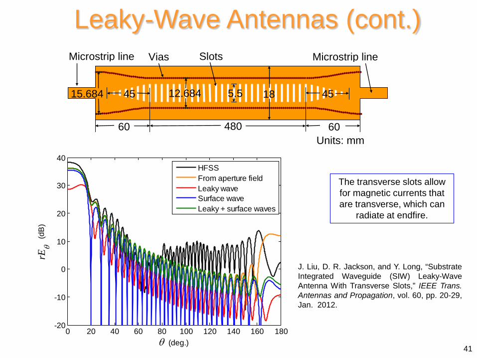
15.684 45 12.684 5.5
480 60 60 Units: mm
Microstrip line
45
Vias Microstrip line
18
Slots
0 20 40 60 80 100 120 140 160 180-20
-10
0
10
20
30
40
θ (deg.)
rEθ (
dB)
HFSSFrom aperture fieldLeaky waveSurface waveLeaky + surface waves
J. Liu, D. R. Jackson, and Y. Long, “Substrate Integrated Waveguide (SIW) Leaky-Wave Antenna With Transverse Slots,” IEEE Trans. Antennas and Propagation, vol. 60, pp. 20-29, Jan. 2012.
Leaky-Wave Antennas (cont.)
The transverse slots allow for magnetic currents that are transverse, which can
radiate at endfire.
42
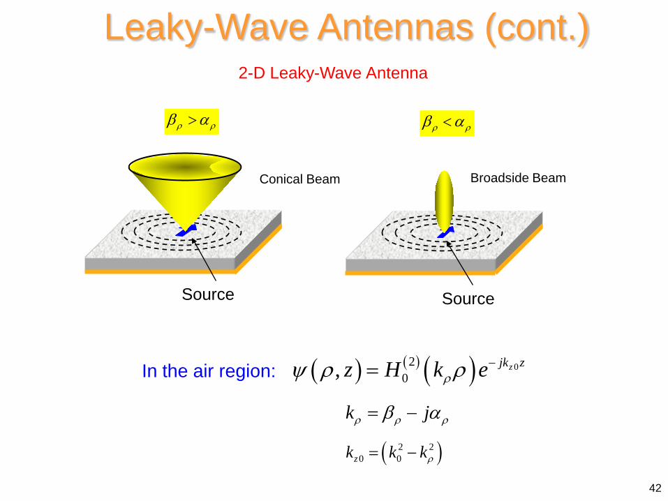
( ) ( ) ( ) 020, zjk zz H k eρψ ρ ρ −=In the air region:
k jρ ρ ρβ α= −
( )2 20 0zk k kρ= −
Leaky-Wave Antennas (cont.)
Broadside Beam
Source
Conical Beam
Source
ρ ρβ α<ρ ρβ α>
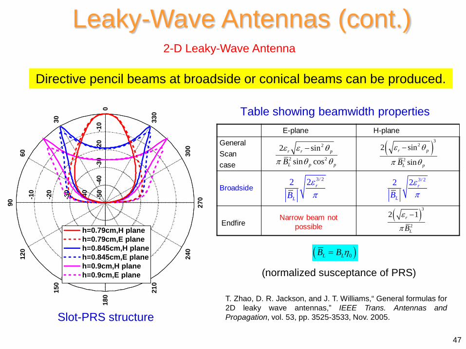
2-D Leaky-Wave Antenna
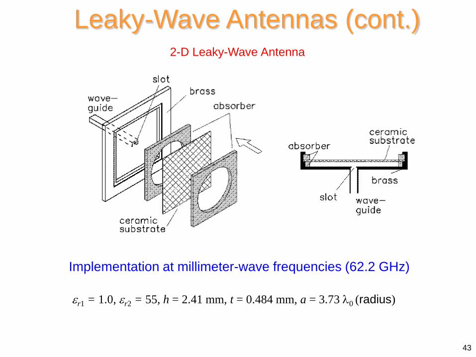
Implementation at millimeter-wave frequencies (62.2 GHz)
εr1 = 1.0, εr2 = 55, h = 2.41 mm, t = 0.484 mm, a = 3.73 λ0 (radius)
43
Leaky-Wave Antennas (cont.) x / λ0
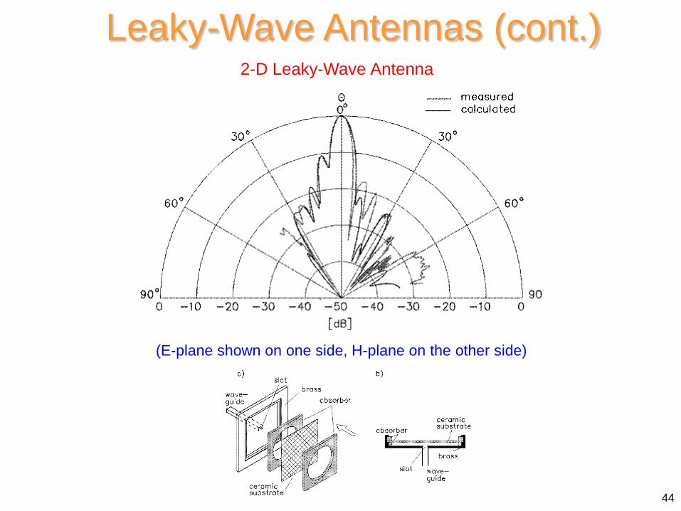
2-D Leaky-Wave Antenna
x / λ0
(E-plane shown on one side, H-plane on the other side)
44
Leaky-Wave Antennas (cont.) 2-D Leaky-Wave Antenna
45
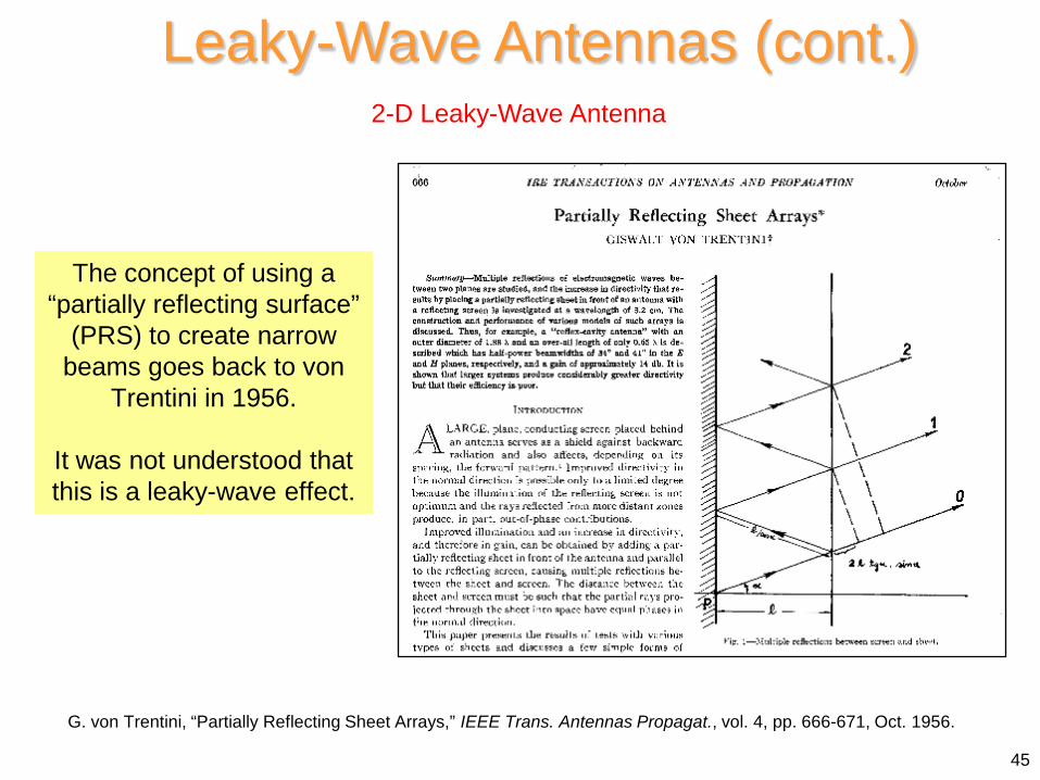
G. von Trentini, “Partially Reflecting Sheet Arrays,” IEEE Trans. Antennas Propagat., vol. 4, pp. 666-671, Oct. 1956.
The concept of using a “partially reflecting surface”
(PRS) to create narrow beams goes back to von
Trentini in 1956.
It was not understood that this is a leaky-wave effect.
Leaky-Wave Antennas (cont.) 2-D Leaky-Wave Antenna
46
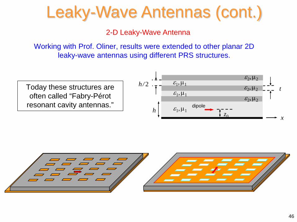
h
t
z0 x ε1, µ1
ε2, µ2 ε1, µ1 ε1, µ1 ε2, µ2
ε2, µ2 h / 2
dipole
Working with Prof. Oliner, results were extended to other planar 2D leaky-wave antennas using different PRS structures.
Today these structures are often called “Fabry-Pérot
resonant cavity antennas.”
Leaky-Wave Antennas (cont.) 2-D Leaky-Wave Antenna
47
0
30
60
90
120
150
180
210
240
270
300
330
-50
-40
-40
-30
-30
-20
-20
-10
-10
h=0.79cm,H planeh=0.79cm,E planeh=0.845cm,H planeh=0.845cm,E planeh=0.9cm,H planeh=0.9cm,E plane
Directive pencil beams at broadside or conical beams can be produced.
E-plane H-planeGeneralScancase
Broadside
EndfireNarrow beam not
possible
3/ 222 r
LBεπ
2
2 2
2 sinsin cos
r r p
L p pBε ε θ
π θ θ
− ( )32
2
2 sin
sinr p
L pB
ε θ
π θ
−
( )3
2
2 1r
LB
ε
π
−
3/ 222 r
LBεπ
( )0L LB B η=
Table showing beamwidth properties
Slot-PRS structure
(normalized susceptance of PRS)
T. Zhao, D. R. Jackson, and J. T. Williams,“ General formulas for 2D leaky wave antennas,” IEEE Trans. Antennas and Propagation, vol. 53, pp. 3525-3533, Nov. 2005.
Leaky-Wave Antennas (cont.) 2-D Leaky-Wave Antenna
x / λ0
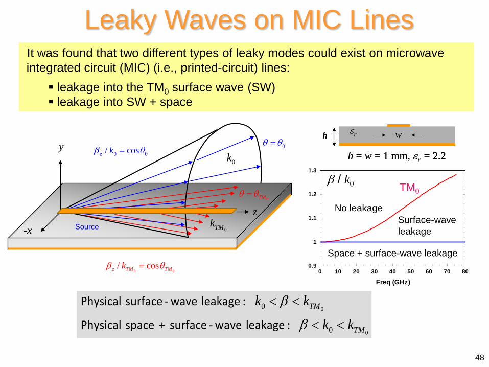
Leaky Waves on MIC Lines
48
0
0
0
0
TM
TM
k k
k k
β
β
< <
< <
Physical surface - wave leakage :
Physical space + surface - wave leakage :
0TMk
0k
Source
y
z
-x
0 10 20 30 40 50 60 70 80
Freq (GHz)
0.9
1
1.1
1.2
1.3
0.9
1
1.1
1.2
1.3
β / k0
Space + surface-wave leakage
Surface-wave leakage
No leakage
TM0
h = w = 1 mm, εr = 2.2
h wεr
h = w = 1 mm, εr = 2.2
h wεrh wwεr
It was found that two different types of leaky modes could exist on microwave integrated circuit (MIC) (i.e., printed-circuit) lines:
leakage into the TM0 surface wave (SW) leakage into SW + space
0 0/ cosz kβ θ=
0 0/ cosz TM TMkβ θ=
0θ θ=
0TMθ θ=
Leaky Waves on MIC Lines (cont.)
49
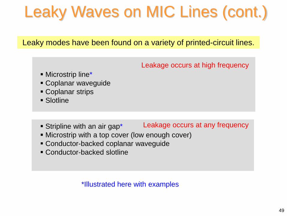
Leaky modes have been found on a variety of printed-circuit lines.
Microstrip line* Coplanar waveguide Coplanar strips Slotline Stripline with an air gap* Microstrip with a top cover (low enough cover) Conductor-backed coplanar waveguide Conductor-backed slotline
Leakage occurs at high frequency
Leakage occurs at any frequency
*Illustrated here with examples
Leaky Waves on MIC Lines (cont.)
50
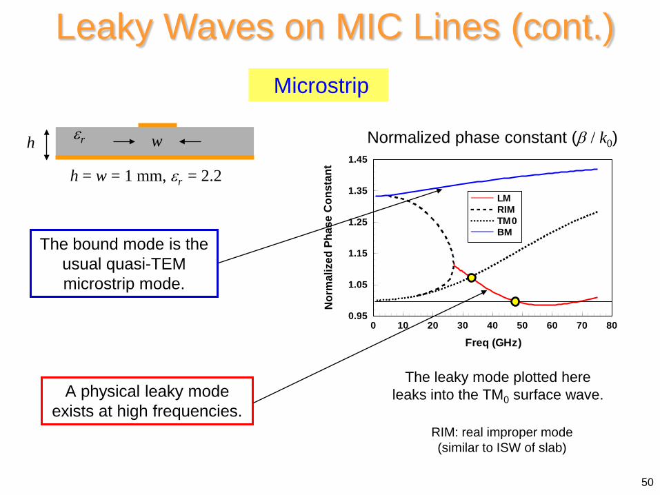
Microstrip
h = w = 1 mm, εr = 2.2
h w εr
A physical leaky mode exists at high frequencies.
The bound mode is the usual quasi-TEM microstrip mode.
The leaky mode plotted here leaks into the TM0 surface wave.
Normalized phase constant (β / k0)
0 10 20 30 40 50 60 70 80
Freq (GHz)
0.95
1.05
1.15
1.25
1.35
1.45
Nor
mal
ized
Pha
se C
onst
ant
LMRIMTM0BM
RIM: real improper mode (similar to ISW of slab)
Leaky Waves on MIC Lines (cont.)
51
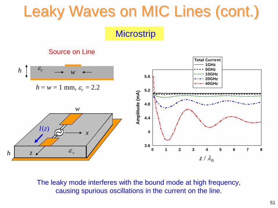
Microstrip
h = w = 1 mm, εr = 2.2
h w εr
The leaky mode interferes with the bound mode at high frequency, causing spurious oscillations in the current on the line.
0 1 2 3 4 5 6 7 8
z/λ0
3.6
4
4.4
4.8
5.2
5.6
Am
plitu
de (m
A)
Total Current1GHz5GHz10GHz20GHz40GHz
z / λ0
w
x
z h rε
I (z)
Source on Line
Leaky Waves on MIC Lines (cont.)
52
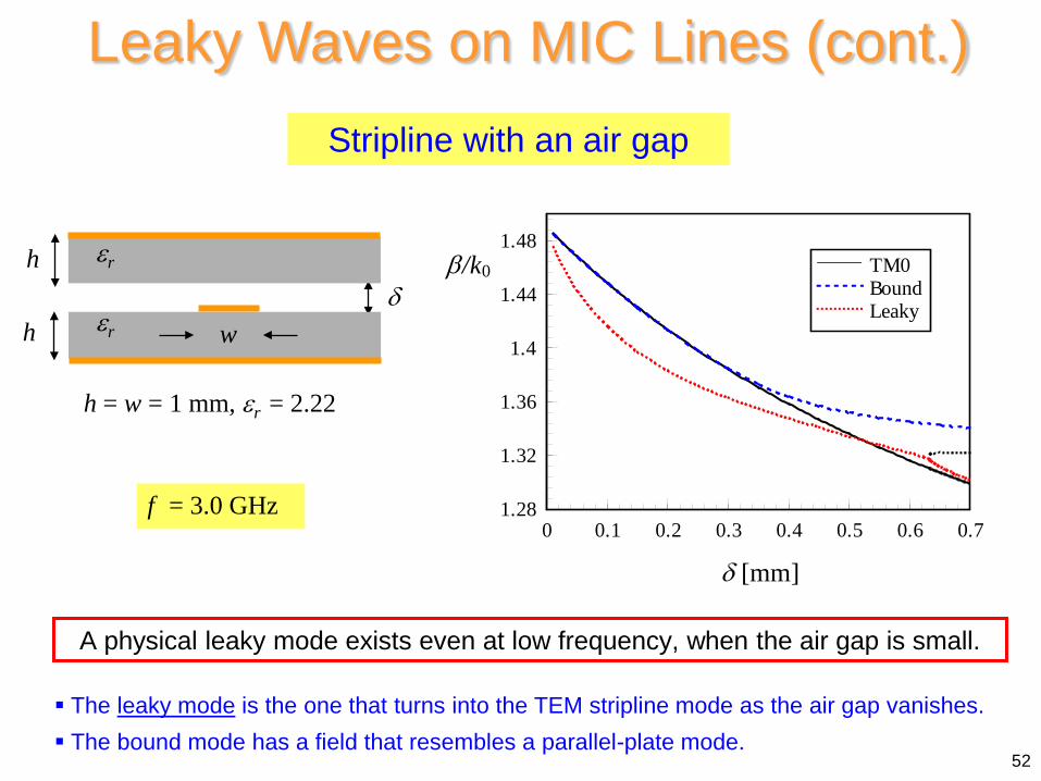
Stripline with an air gap
h = w = 1 mm, εr = 2.22
h δ
h εr
w εr
0 0.1 0.2 0.3 0.4 0.5 0.6 0.71.28
1.32
1.36
1.4
1.44
1.48TM0BoundLeaky
β/k0
δ [mm]
A physical leaky mode exists even at low frequency, when the air gap is small.
f = 3.0 GHz
The leaky mode is the one that turns into the TEM stripline mode as the air gap vanishes. The bound mode has a field that resembles a parallel-plate mode.
Leaky Waves on MIC Lines (cont.)
53
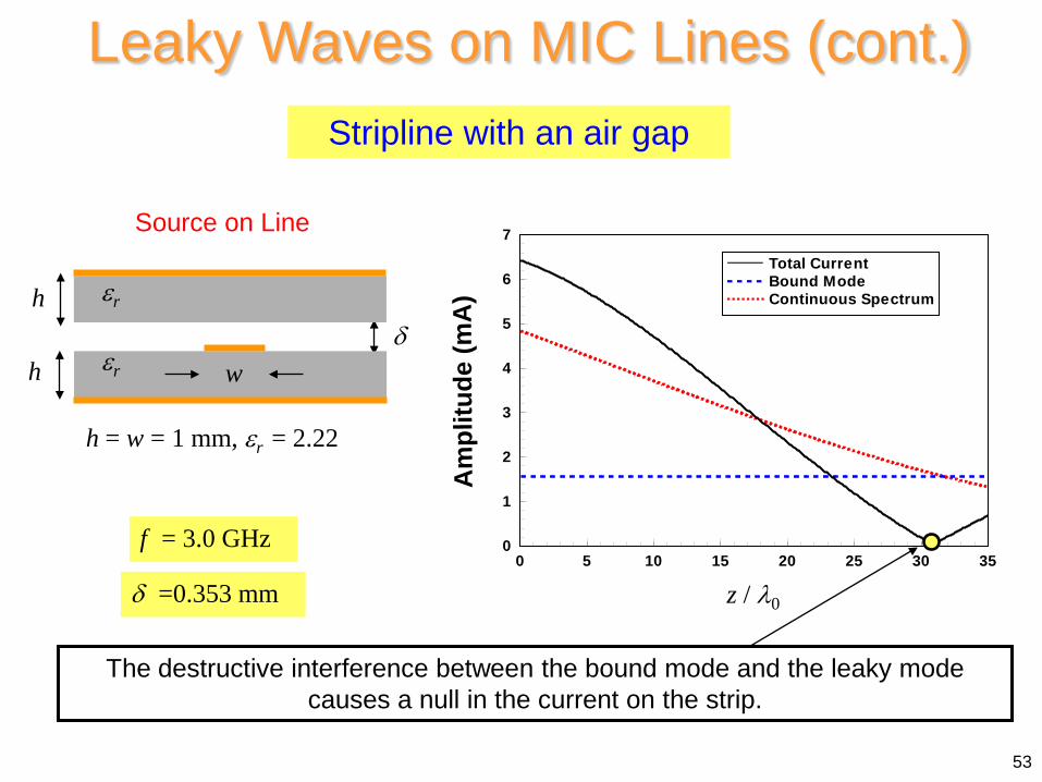
h = w = 1 mm, εr = 2.22
The destructive interference between the bound mode and the leaky mode causes a null in the current on the strip.
δ =0.353 mm 0 5 10 15 20 25 30 35
z/λ0
0
1
2
3
4
5
6
7
Am
plitu
de (m
A)
Total CurrentBound ModeContinuous Spectrum
z / λ0
h δ
h εr
w εr
f = 3.0 GHz
Stripline with an air gap
Source on Line
Leaky Waves on MIC Lines (cont.)
54
F. Mesa and D. R. Jackson, “Leaky Modes and High-Frequency Effects in Microwave Integrated Circuits,” article in Encyclopedia of RF and Microwave Engineering, John Wiley & Sons, Inc., 2005.
References
D. Nghiem, J. T. Williams, D. R. Jackson, and A. A. Oliner, “Leakage of Dominant Mode on Stripline with a Small Air Gap,” IEEE Trans. Microwave Theory and Techniques, Vol. 43, No. 11, pp. 2549-2556, Nov. 1995.
D. Nghiem, J. T. Williams, D. R. Jackson, and A. A. Oliner, “Existence of a Leaky Dominant Mode on Microstrip Line with an Isotropic Substrate: Theory and Measurements,” IEEE Trans. Microwave Theory and Techniques, Vol. 44, No. 10, pp. 1710-1715, Oct. 1996.
M. Freire, F. Mesa, C. Di Nallo, D. R. Jackson, and A. A. Oliner, “Spurious Transmission Effects due to the Excitation of the Bound Mode and the Continuous Spectrum on Stripline with an Air Gap,” IEEE Trans. Microwave Theory and Techniques, Vol. 47, No. 12, pp. 2493-2502, Dec. 1999.
F. Mesa, D. R. Jackson, and M. Freire, “High Frequency Leaky-Mode Excitation on a Microstrip Line,” IEEE Trans. Microwave Theory and Techniques, Vol. 49, No. 12, pp. 2206-2215, Dec. 2001.