ECE 6340 Intermediate EM Waves - University of Houstoncourses.egr.uh.edu/ECE/ECE6340/Class...

Prof. David R. Jackson Dept. of ECE

Fall 2016

Notes 7

ECE 6340 Intermediate EM Waves

1

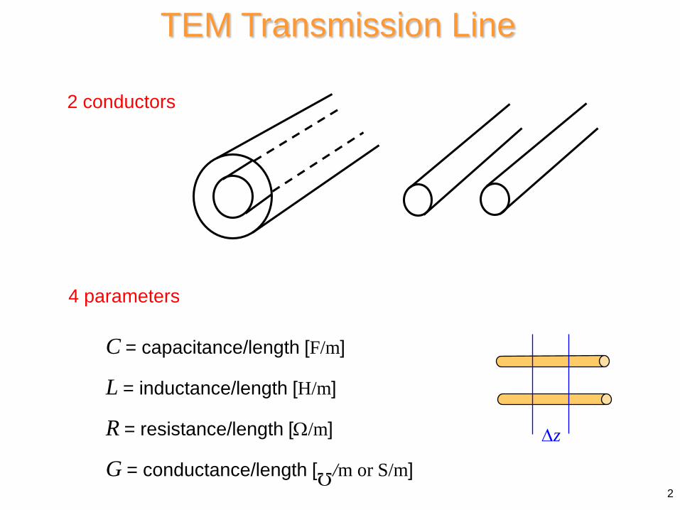
TEM Transmission Line

2 conductors

4 parameters

C = capacitance/length [F/m]

L = inductance/length [H/m]

R = resistance/length [Ω/m]

G = conductance/length [ /m or S/m] Ω

∆z

2

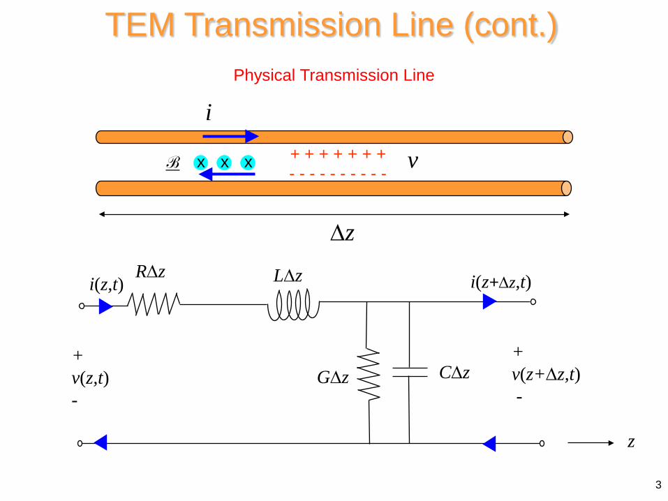
TEM Transmission Line (cont.)

z∆

i+ + + + + + + - - - - - - - - - -

vx x x B

3

Physical Transmission Line

+ v(z,t) -

R∆z L∆z

G∆z C∆z

i(z,t)

+ v(z+∆z,t) -

i(z+∆z,t)

z

( , )( , ) ( , ) ( , )

( , )( , ) ( , ) ( , )

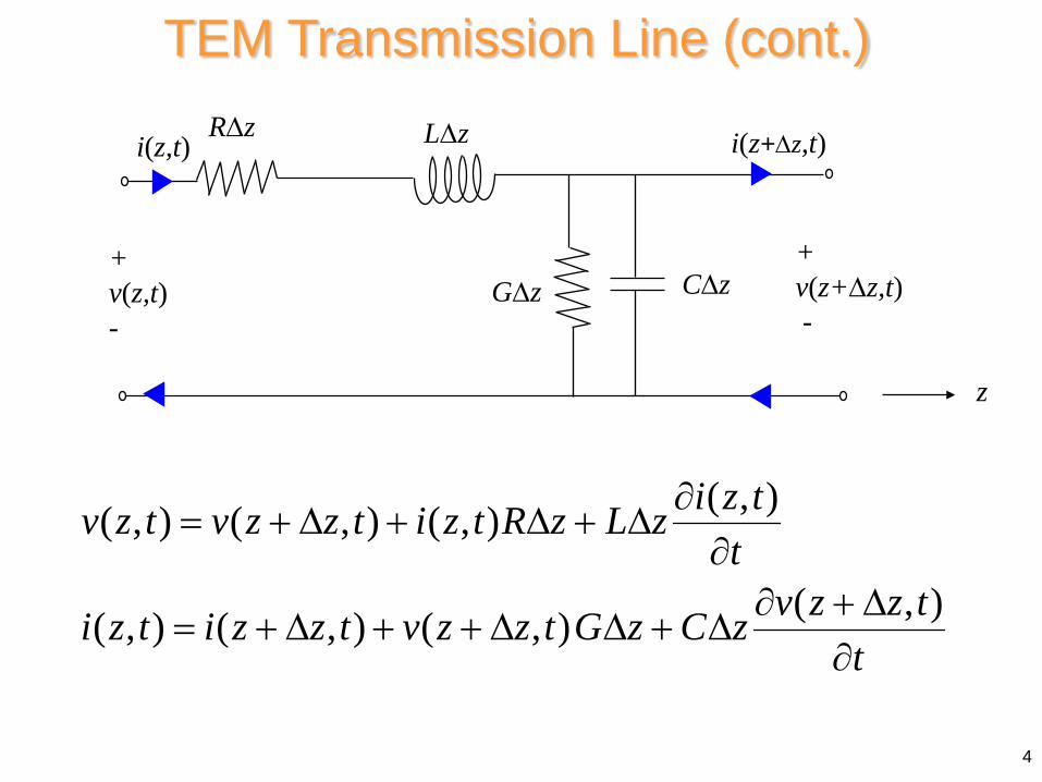
i z tv z t v z z t i z t R z L zt

v z z ti z t i z z t v z z t G z C zt

∂= + ∆ + ∆ + ∆

∂∂ + ∆

= + ∆ + + ∆ ∆ + ∆∂


4

+ v(z,t) -

R∆z L∆z

G∆z C∆z

i(z,t)

+ v(z+∆z,t) -

i(z+∆z,t)

z

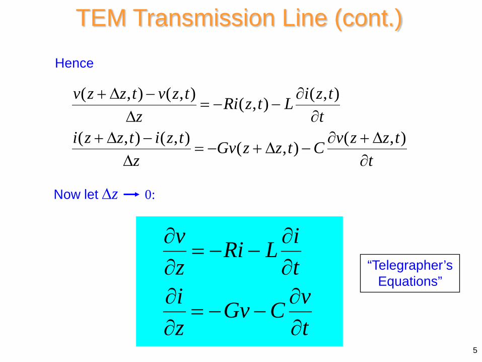
Hence

( , ) ( , ) ( , )( , )

( , ) ( , ) ( , )( , )

v z z t v z t i z tRi z t Lz t

i z z t i z t v z z tGv z z t Cz t

+ ∆ − ∂= − −

∆ ∂+ ∆ − ∂ + ∆

= − + ∆ −∆ ∂

Now let ∆z 0:

v iRi Lz ti vGv Cz t

∂ ∂= − −

∂ ∂∂ ∂

= − −∂ ∂

“Telegrapher’sEquations”


5

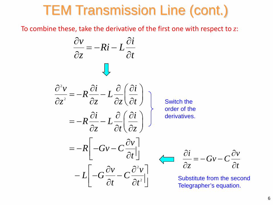
To combine these, take the derivative of the first one with respect to z:

2

2

2

2

v i iR Lz z z t

i iR Lz t z

vR Gv Ct

v vL G Ct t

∂ ∂ ∂ ∂ = − − ∂ ∂ ∂ ∂ ∂ ∂ ∂ = − − ∂ ∂ ∂

∂ = − − − ∂ ∂ ∂ − − − ∂ ∂

Switch the order of the derivatives.


6

v iRi Lz t∂ ∂

= − −∂ ∂

i vGv Cz t∂ ∂

= − −∂ ∂

Substitute from the second Telegrapher’s equation.

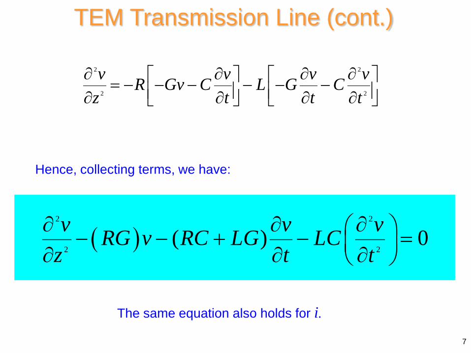
( )2 2

2 2( ) 0v v vRG v RC LG LC

z t t∂ ∂ ∂ − − + − = ∂ ∂ ∂

The same equation also holds for i.

Hence, collecting terms, we have:

2 2

2 2

v v v vR Gv C L G Cz t t t∂ ∂ ∂ ∂ = − − − − − − ∂ ∂ ∂ ∂


7

( )2

2

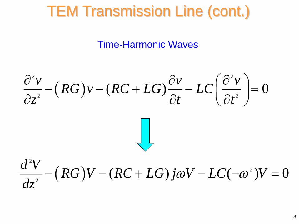
2( ) ( ) 0d V RG V RC LG j V LC V

dzω ω− − + − − =

( )2 2

2 2( ) 0v v vRG v RC LG LC

z t t∂ ∂ ∂ − − + − = ∂ ∂ ∂


Time-Harmonic Waves

8

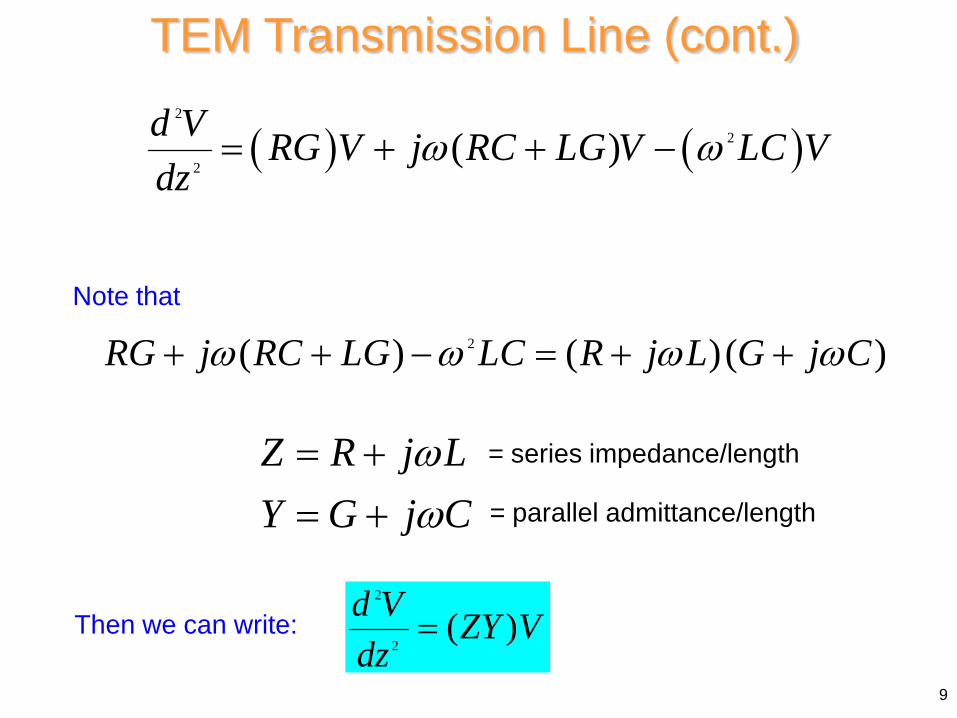
Note that

= series impedance/length

( ) ( )2

2

2( )d V RG V j RC LG V LC V

dzω ω= + + −

2( ) ( )( )RG j RC LG LC R j L G j Cω ω ω ω+ + − = + +

Z R j LY G j C

ωω

= += + = parallel admittance/length

Then we can write: 2

2( )d V ZY V

dz=


9

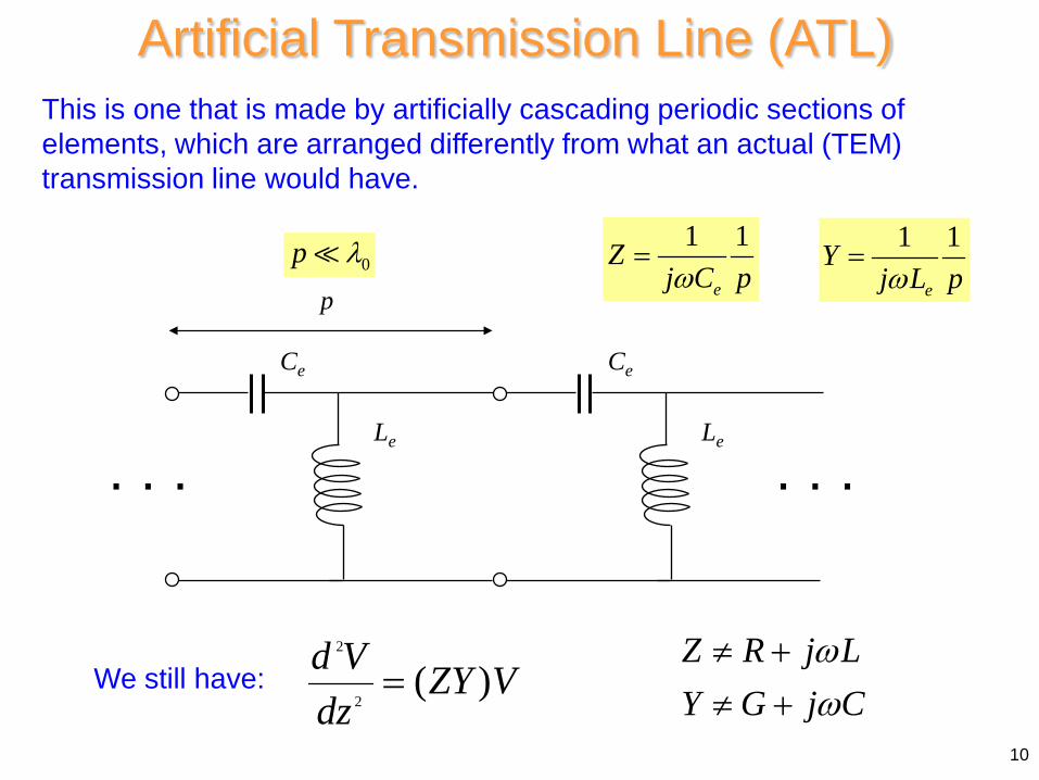
This is one that is made by artificially cascading periodic sections of elements, which are arranged differently from what an actual (TEM) transmission line would have.

We still have: 2

2( )d V ZY V

dz=

Artificial Transmission Line (ATL)

Z R j LY G j C

ωω

≠ +≠ +

1 1

e

Zj C pω

= 1 1

e

Yj L pω

=

10

0p λ

Ce

Le

Ce

Le

. . . . . .

p

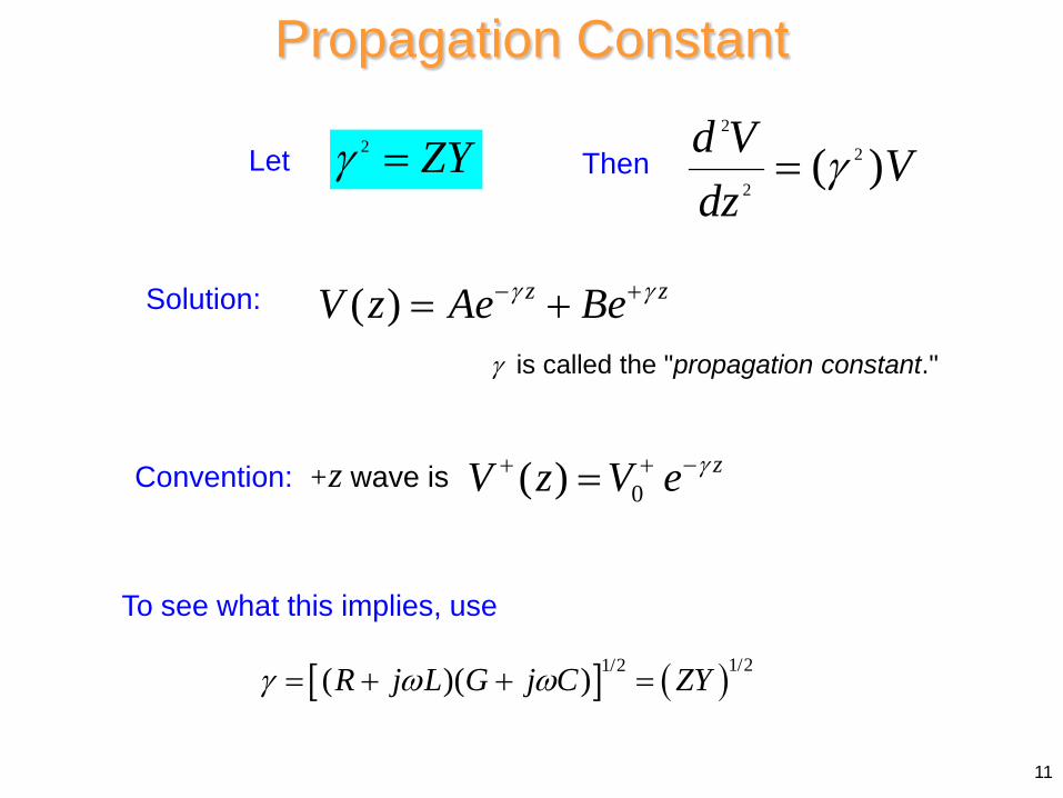
Let

Convention: +z wave is

Solution:

2γ = ZY

( ) z zV z Ae Beγ γ− += +

0( ) zV z V e γ+ + −=

[ ] ( )1/21/2( )( )R j L G j C ZYγ ω ω= + + =

To see what this implies, use

2

2

2( )d V V

dzγ=Then

Propagation Constant

γ is called the "propagation constant."

11

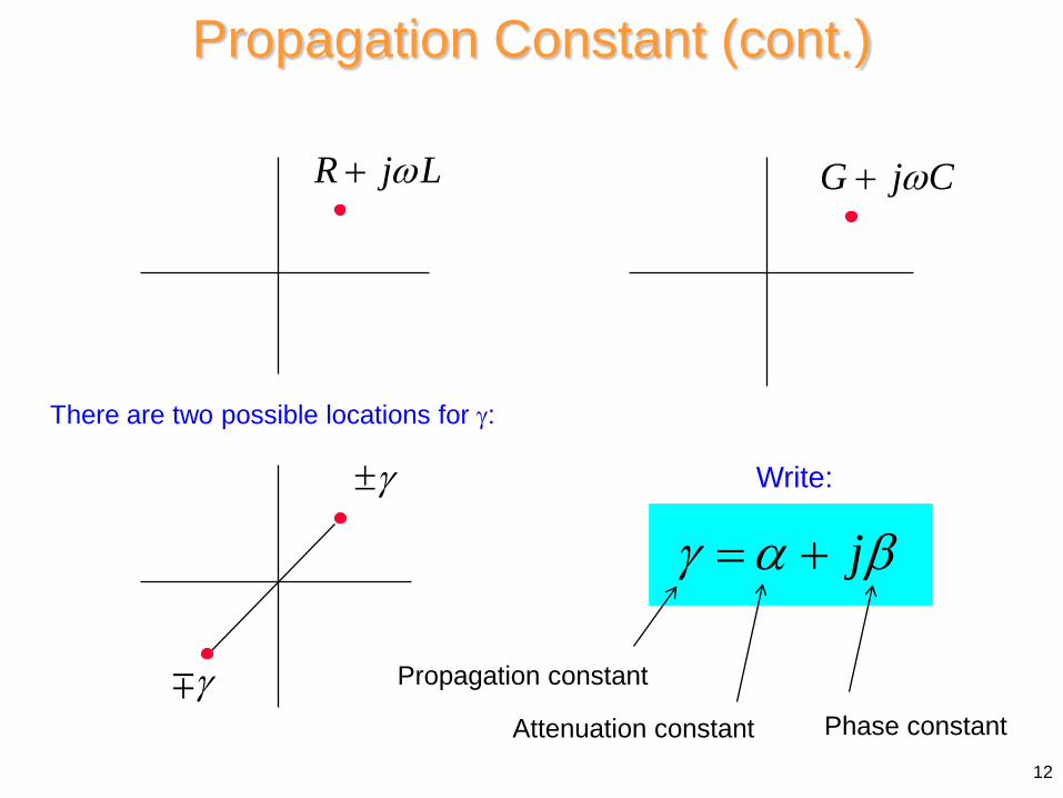
Write:

R j Lω+ G j Cω+

γ±

γ

jγ α β= +

There are two possible locations for γ:

Attenuation constant Phase constant

Propagation constant

12

Propagation Constant (cont.)

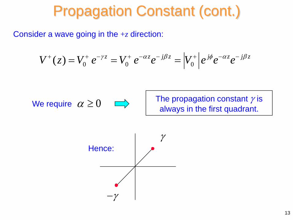
0 0 0( ) z z j z j z j zV z V e V e e V e e eγ α β φ α β+ + − + − − + − −= = =

We require 0α ≥

Hence:

γ

γ−

The propagation constant γ is always in the first quadrant.

13

Propagation Constant (cont.) Consider a wave going in the +z direction:

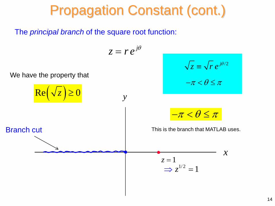
The principal branch of the square root function:

π θ π− < ≤

14


/2jz r e θ≡

jz r e θ=

x

Branch cut

y

π θ π− < ≤

1z =1/2 1z⇒ =

( )Re 0z ≥

This is the branch that MATLAB uses.

We have the property that

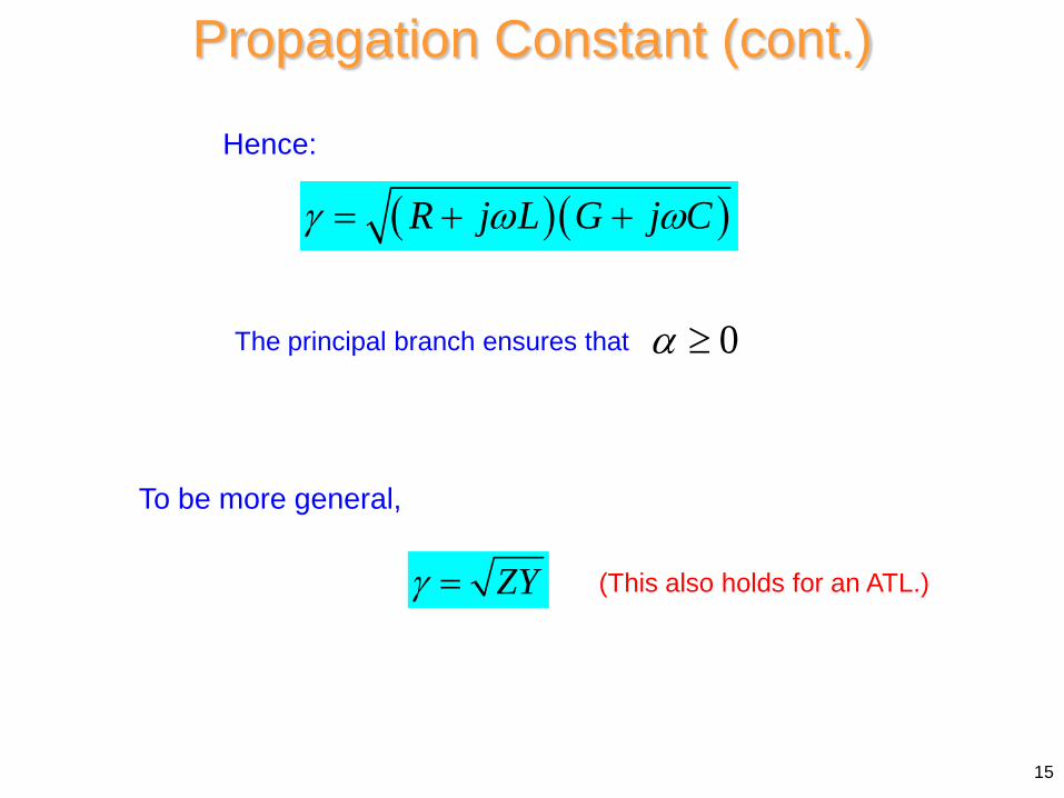
To be more general,

0α ≥

ZYγ =

15


(This also holds for an ATL.)

The principal branch ensures that

( )( )R j L G j Cγ ω ω= + +

Hence:

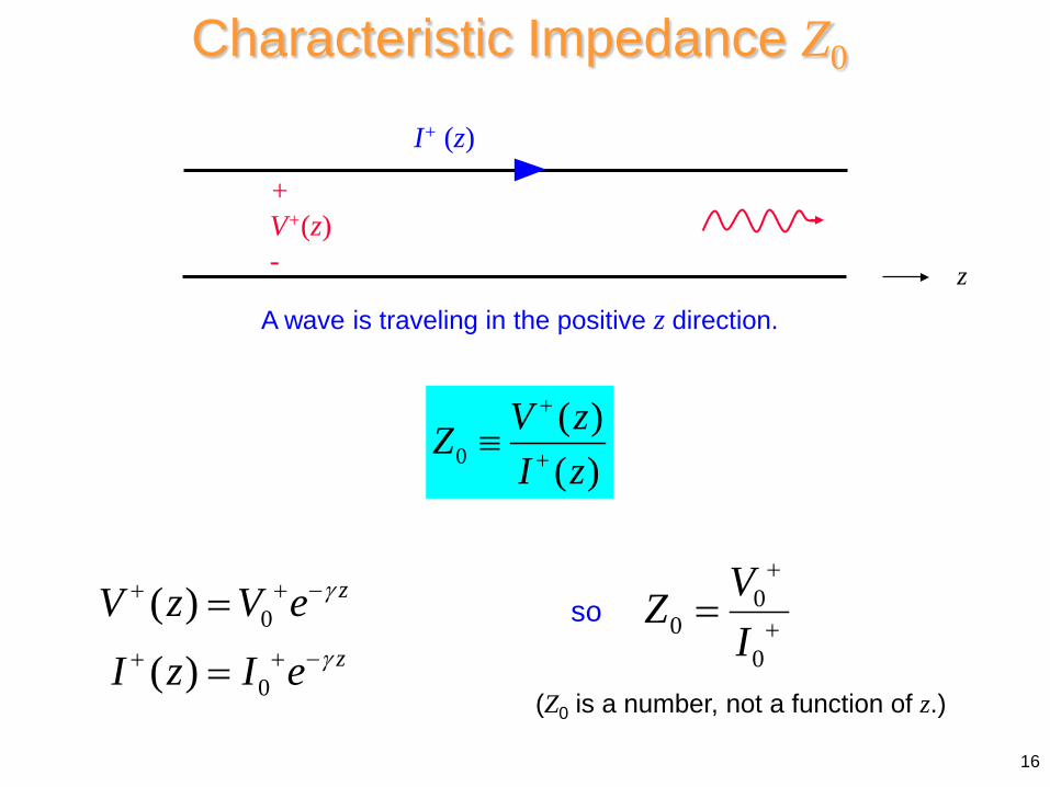
Characteristic Impedance Z0

0( )( )

V zZI z

+

+≡

0

0

( )

( )

z

z

V z V eI z I e

γ

γ

+ + −

+ + −

=

=so 0

00

VZI

+

+=

+ V+(z) -

I+ (z)

z

A wave is traveling in the positive z direction.

(Z0 is a number, not a function of z.)

16

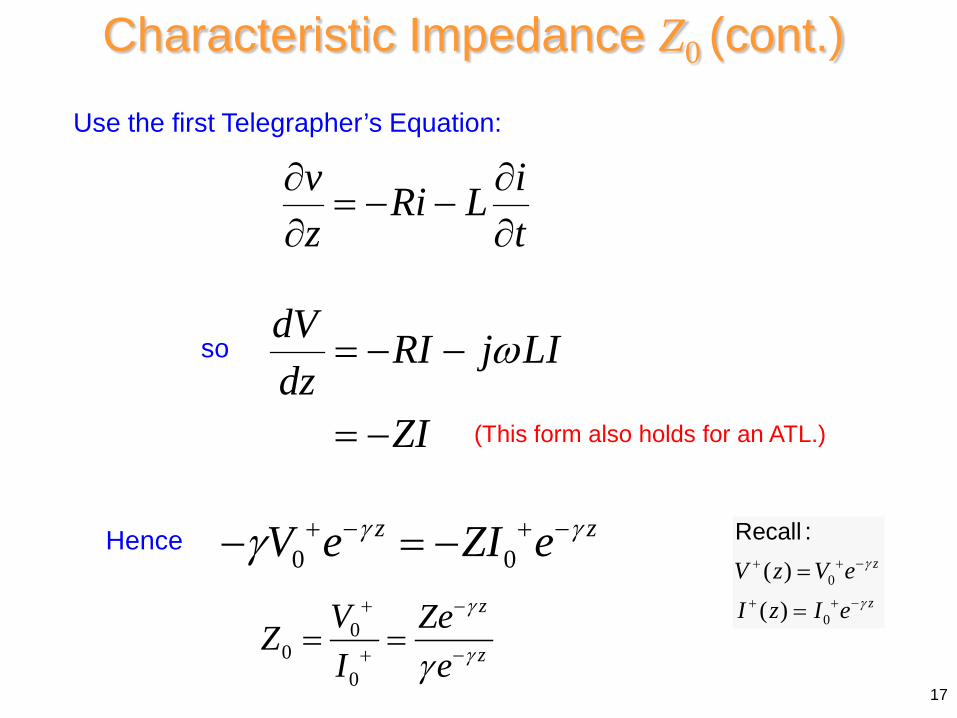
Use the first Telegrapher’s Equation:

v iRi Lz t∂ ∂

= − −∂ ∂

so dV RI j LIdz

ZI

ω= − −

= −

Hence 0 0

z zV e ZI eγ γγ + − + −− = −

Characteristic Impedance Z0 (cont.)

17

00

0

z

z

V ZeZI e

γ

γγ

+ −

+ −= =

(This form also holds for an ATL.)

0

0

( )

( )

z

z

V z V eI z I e

γ

γ

+ + −

+ + −

=

=

Recall :

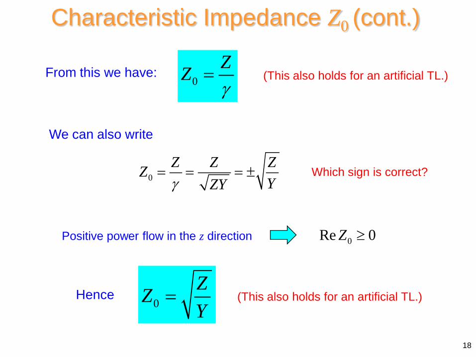
From this we have: 0

ZZγ

=


18

0Z Z ZZ

YZYγ= = = ±

(This also holds for an artificial TL.)

We can also write

Which sign is correct?

0Re 0Z ≥Positive power flow in the z direction

0ZZY

=Hence (This also holds for an artificial TL.)


19

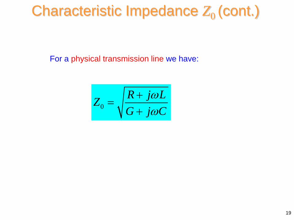
For a physical transmission line we have:

0R j LZG j C

ωω

+=

+

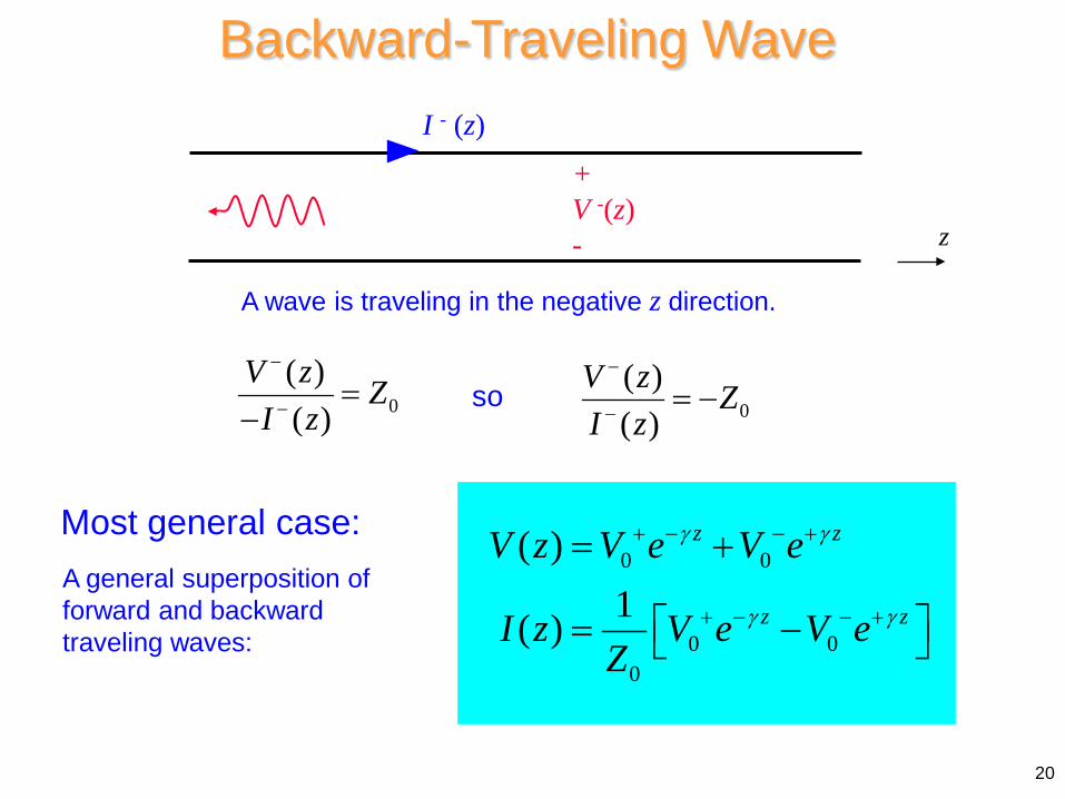
Backward-Traveling Wave

0( )( )

V z ZI z

−

− =− 0

( )( )

V z ZI z

−

− = −so

0 0

0 00

( )1( )

z z

z z

V z V e V e

I z V e V eZ

γ γ

γ γ

+ − − +

+ − − +

= +

= −

+ V -(z) -

I - (z)

z

A general superposition of forward and backward traveling waves:

Most general case:

A wave is traveling in the negative z direction.

20

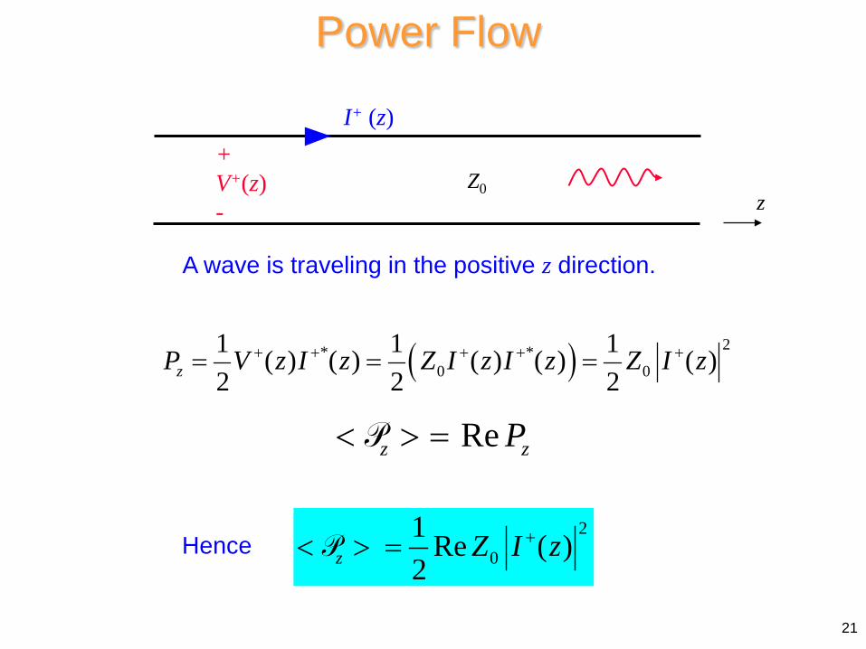
Power Flow

( ) 2* *0 0

1 1 1( ) ( ) ( ) ( ) ( )2 2 2zP V z I z Z I z I z Z I z+ + + + += = =

Rez zP< > =P

Hence

+ V+(z) -

I+ (z)

Z0 z

2

01 Re ( )2z Z I z+< > =P

A wave is traveling in the positive z direction.

21

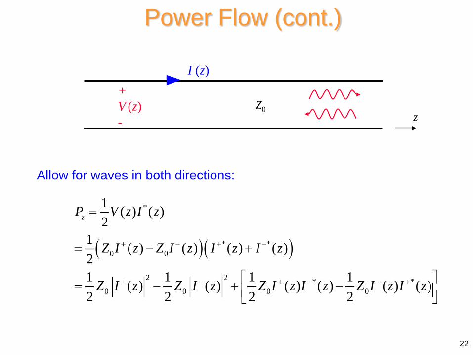
Power Flow (cont.)

( )( )

*

* *0 0

2 2 * *0 0 0 0

1 ( ) ( )2

1 ( ) ( ) ( ) ( )21 1 1 1( ) ( ) ( ) ( ) ( ) ( )2 2 2 2

zP V z I z

Z I z Z I z I z I z

Z I z Z I z Z I z I z Z I z I z

+ − + −

+ − + − − +

=

= − +

= − + −

+ V (z) -

I (z)

Z0 z

Allow for waves in both directions:

22

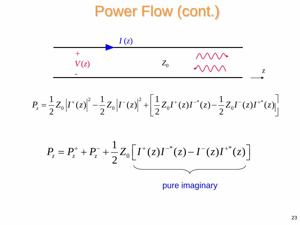
2 2 * *0 0 0 0

1 1 1 1( ) ( ) ( ) ( ) ( ) ( )2 2 2 2zP Z I z Z I z Z I z I z Z I z I z+ − + − − + = − + −

* *0

1 ( ) ( ) ( ) ( )2z z zP P P Z I z I z I z I z+ − + − − + = + + −

pure imaginary

Power Flow (cont.)

+ V (z) -

I (z)

Z0 z

23

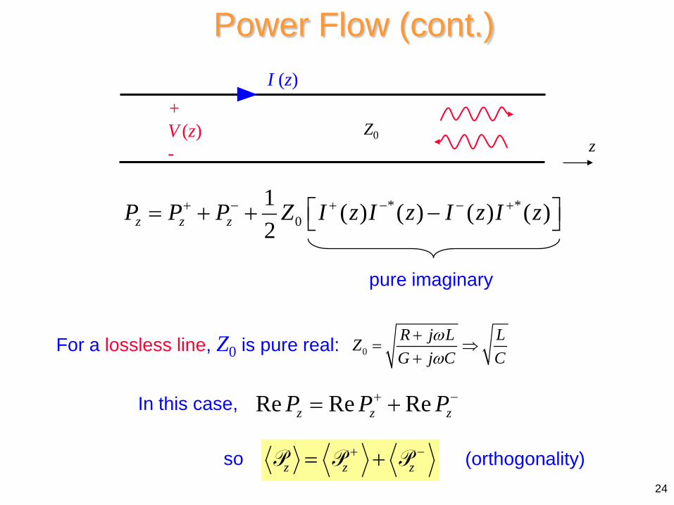
* *0

1 ( ) ( ) ( ) ( )2z z zP P P Z I z I z I z I z+ − + − − + = + + −

pure imaginary

For a lossless line, Z0 is pure real:

In this case, Re Re Rez z zP P P+ −= +

z z z+ −= +P P Pso (orthogonality)

Power Flow (cont.)

+ V (z) -

I (z)

Z0 z

0R j L LZG j C C

ωω

+= ⇒

+

24

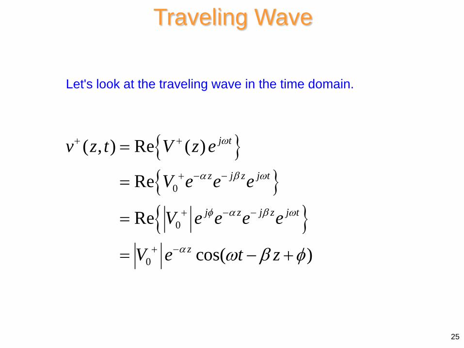
Traveling Wave

0

0

0

( , ) Re ( )

Re

Re

cos( )

j t

z j z j t

j z j z j t

z

v z t V z e

V e e e

V e e e e

V e t z

ω

α β ω

φ α β ω

α ω β φ

+ +

+ − −

+ − −

+ −

=

=

=

= − +

Let's look at the traveling wave in the time domain.

25

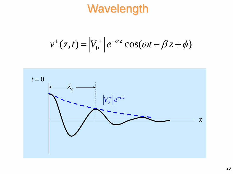
Wavelength

0( , ) cos( )zv z t V e t zα ω β φ+ + −= − +

gλ0t =

z

0zV e α+ −

26

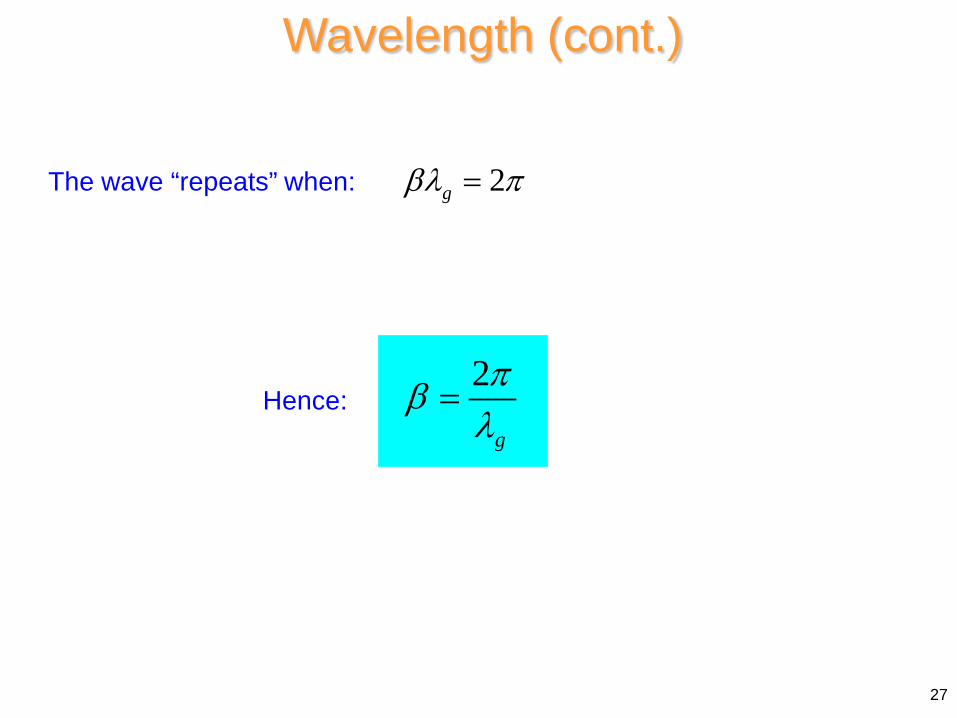
Wavelength (cont.)

2

g

πβλ

=

2gβλ π=The wave “repeats” when:

Hence:

27

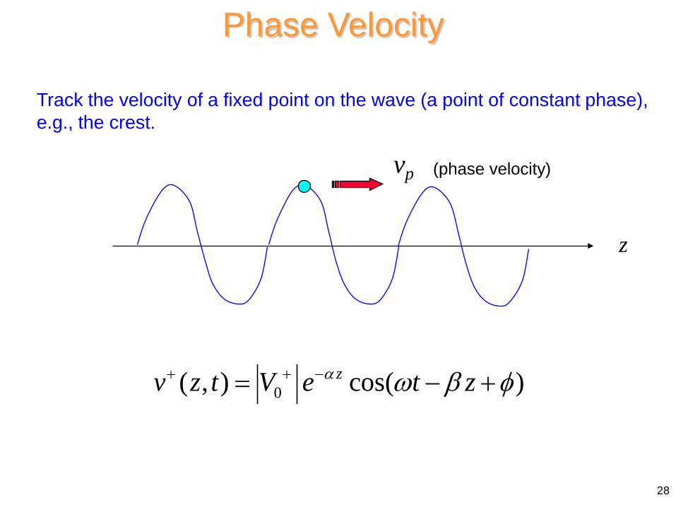
Phase Velocity

Track the velocity of a fixed point on the wave (a point of constant phase), e.g., the crest.

0( , ) cos( )zv z t V e t zα ω β φ+ + −= − +

z

vp (phase velocity)

28

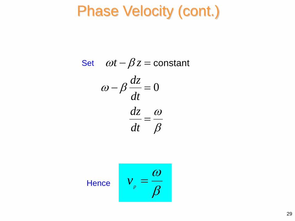
Phase Velocity (cont.)

0

t zdzdtdzdt

ω β

ω β

ωβ

− =

− =

=

constantSet

Hence pv ω

β=

29

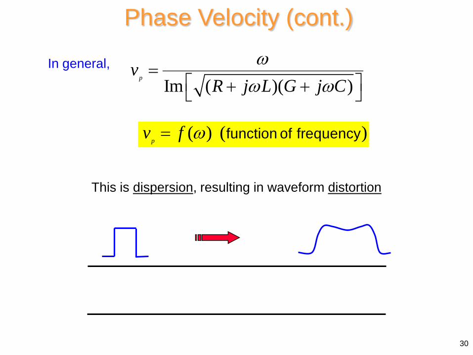
In general,

Im ( )( )p

vR j L G j C

ωω ω

= + +

This is dispersion, resulting in waveform distortion

Phase Velocity (cont.)

( ) ( )p

v f ω= function of frequency

30

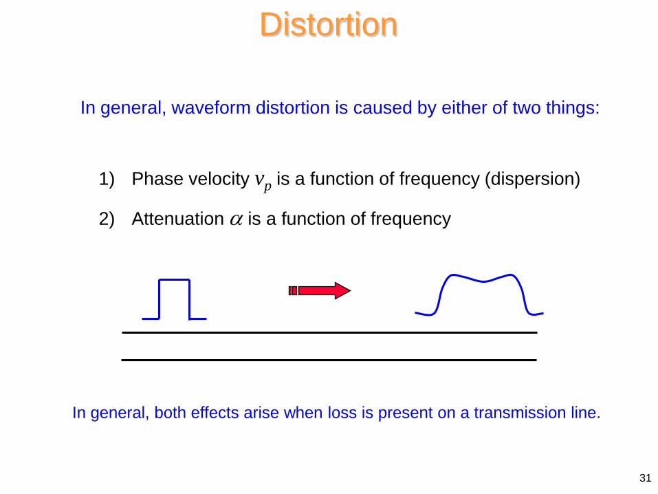
In general, waveform distortion is caused by either of two things:

Distortion

1) Phase velocity vp is a function of frequency (dispersion)

2) Attenuation α is a function of frequency

In general, both effects arise when loss is present on a transmission line.

31

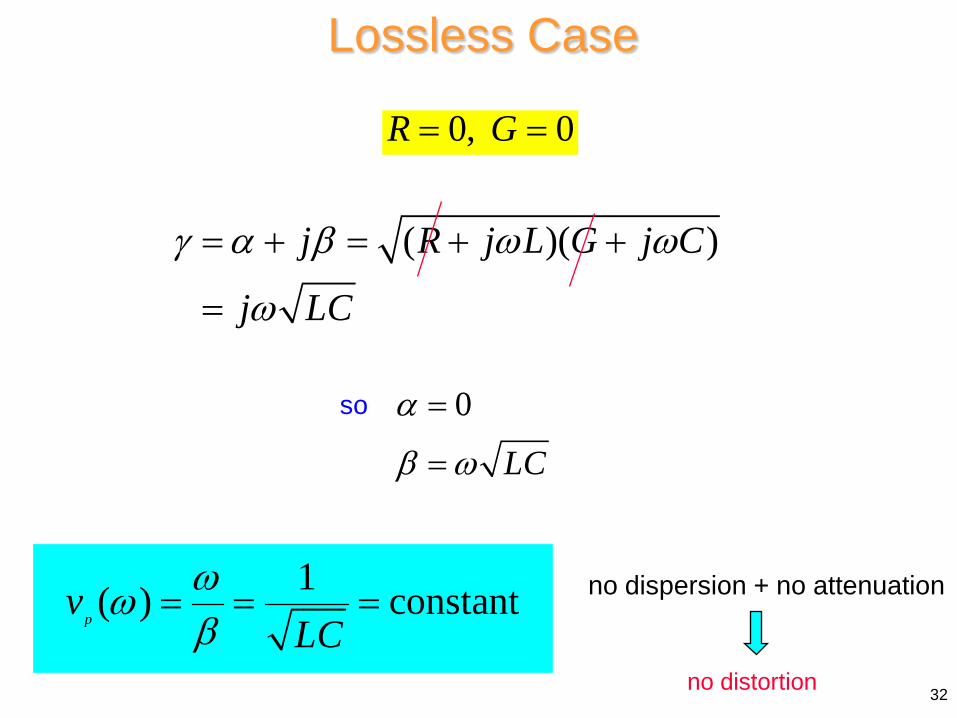
Lossless Case

0, 0R G= =

( )( )j R j L G j C

j LC

γ α β ω ω

ω

= + = + +

=

so 0

LC

α

β ω

=

=

1( ) constantp

vLC

ωωβ

= = = no dispersion + no attenuation

no distortion 32

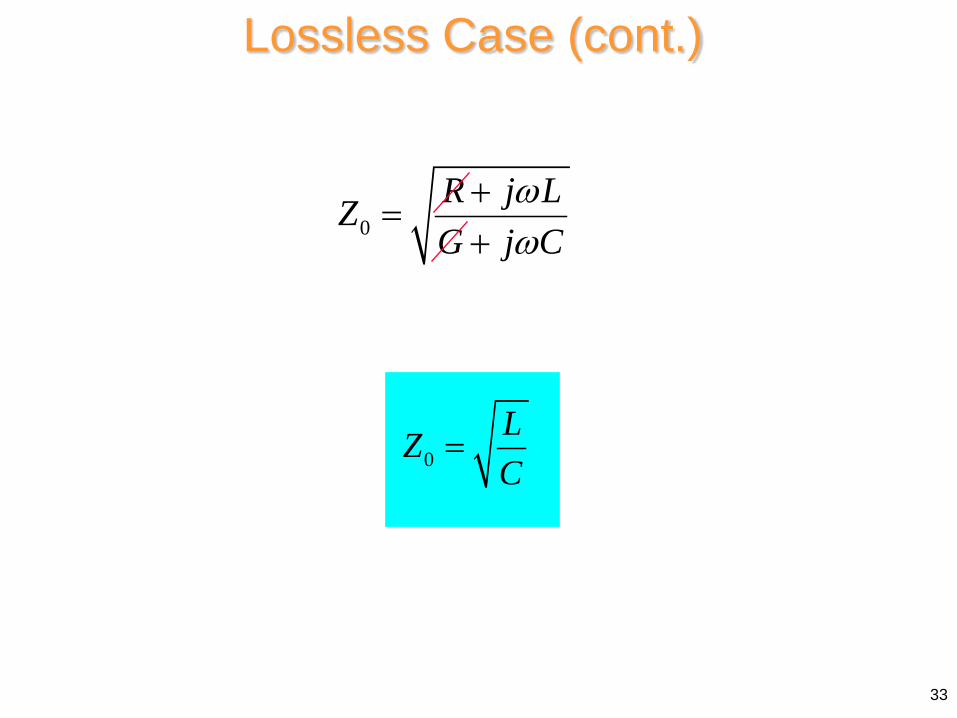
Lossless Case (cont.)

0R j LZG j C

ωω

+=

+

0LZC

=

33

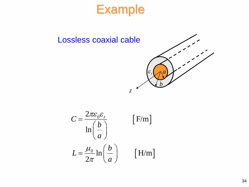
Example

Lossless coaxial cable

[ ]

[ ]

0

0

2 F/mln

ln H/m2

rCba

bLa

πε ε

µπ

=

=

rε a

b z

34

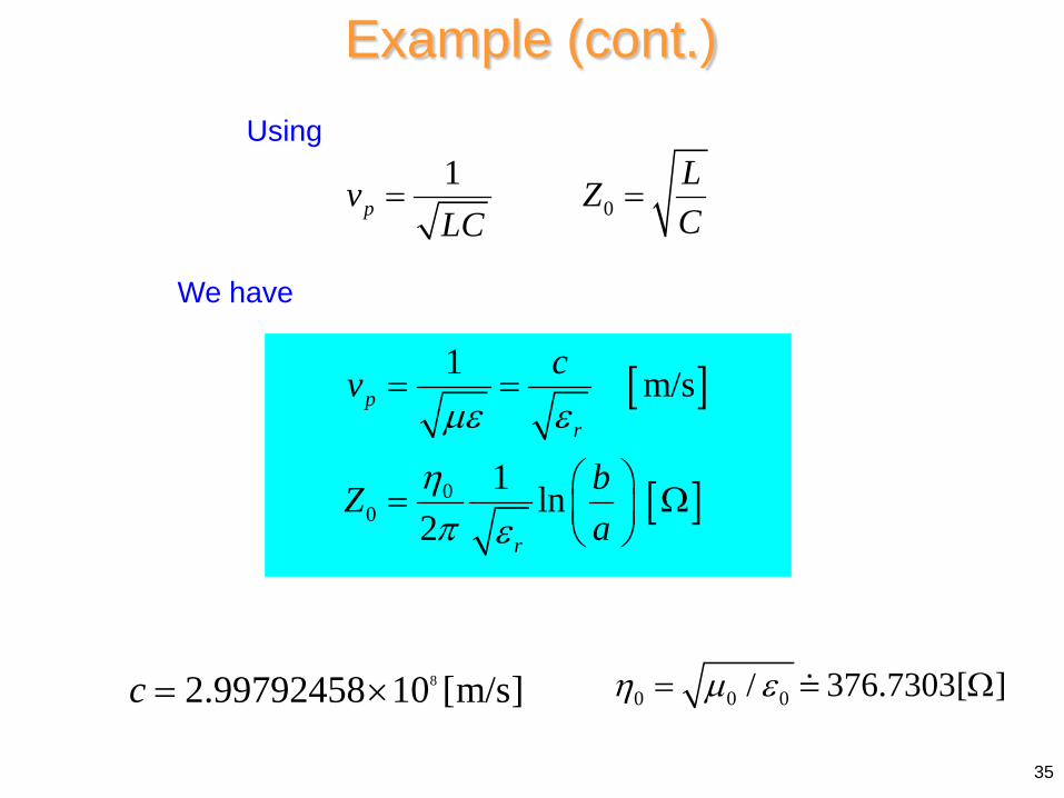
Example (cont.)

01

pLv ZCLC

= =

[ ]

[ ]00

1 m/s

1 ln2

pr

r

cv

bZa

µε ε

ηπ ε

= =

= Ω

82.99792458 10 [m/s]c = × 0 0 0/ 376.7303[ ]η µ ε= Ω

Using

We have

35

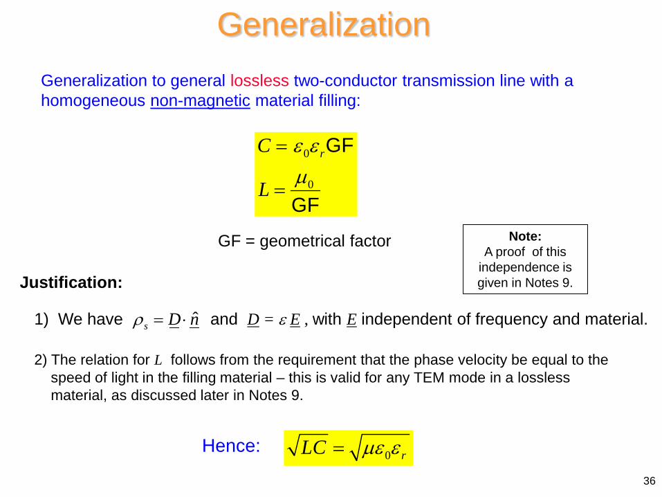
Generalization Generalization to general lossless two-conductor transmission line with a homogeneous non-magnetic material filling:

0

0

rC

L

ε εµ

=

=

GF

GF

2) The relation for L follows from the requirement that the phase velocity be equal to the speed of light in the filling material – this is valid for any TEM mode in a lossless material, as discussed later in Notes 9.

GF = geometrical factor

1) We have and D = ε E , with E independent of frequency and material. ˆs D nρ = ⋅

0 rLC µε ε=36

Hence:

Note: A proof of this

independence is given in Notes 9. Justification:

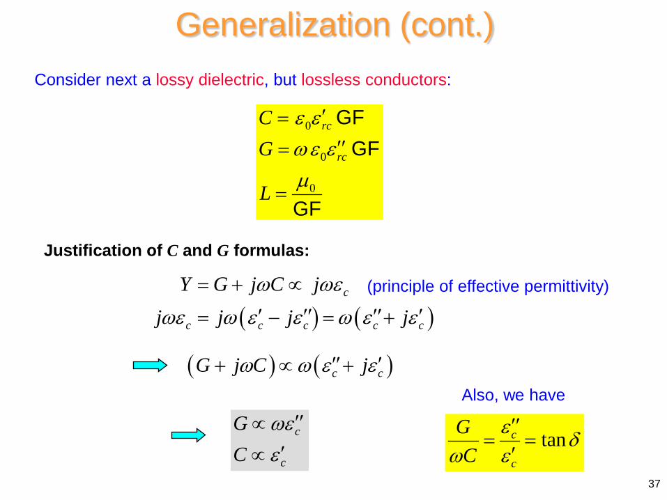
Generalization (cont.) Consider next a lossy dielectric, but lossless conductors:

0

0

0

rc

rc

CG

L

ε εωε εµ

′=′′=

=

GFGF

GF

( ) ( )c

c c c c c

Y G j C jj j j j

ω ωε

ωε ω ε ε ω ε ε

= + ∝

′ ′′ ′′ ′= − = +

c

c

GC

ωεε

′′∝′∝

37

Justification of C and G formulas:

( ) ( )c cG j C jω ω ε ε′′ ′+ ∝ +

tanc

c

GC

ε δω ε

′′= =

′

(principle of effective permittivity)

Also, we have

Generalization (cont.)

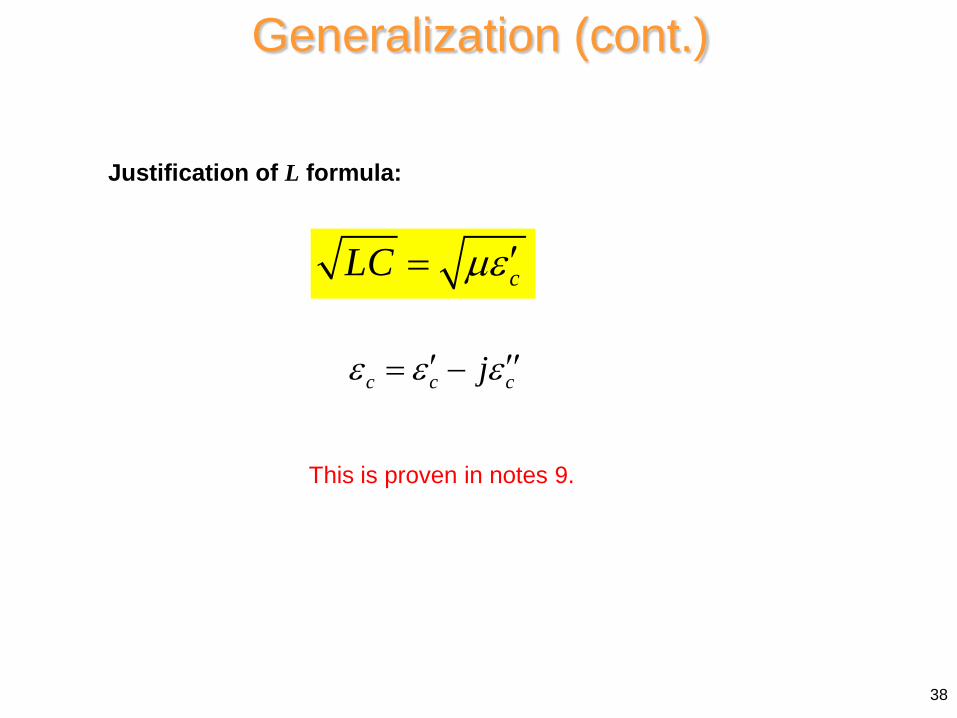
cLC µε ′=

This is proven in notes 9.

38

Justification of L formula:

c c cjε ε ε′ ′′= −

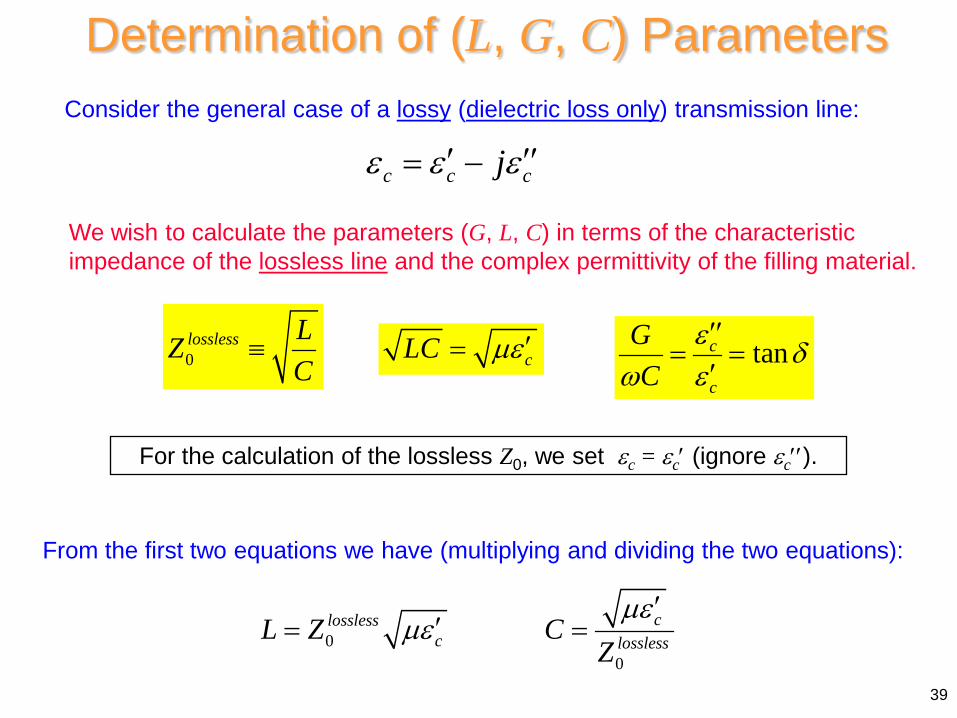
Determination of (L, G, C) Parameters Consider the general case of a lossy (dielectric loss only) transmission line:

tanc

c

GC

ε δω ε

′′= =

′cLC µε ′=0

lossless LZC

≡

From the first two equations we have (multiplying and dividing the two equations):

00

closslessc losslessL Z C

Zµε

µε′

′= =

For the calculation of the lossless Z0, we set εc = εc′ (ignore εc′′).

c c cjε ε ε′ ′′= −

We wish to calculate the parameters (G, L, C) in terms of the characteristic impedance of the lossless line and the complex permittivity of the filling material.

39

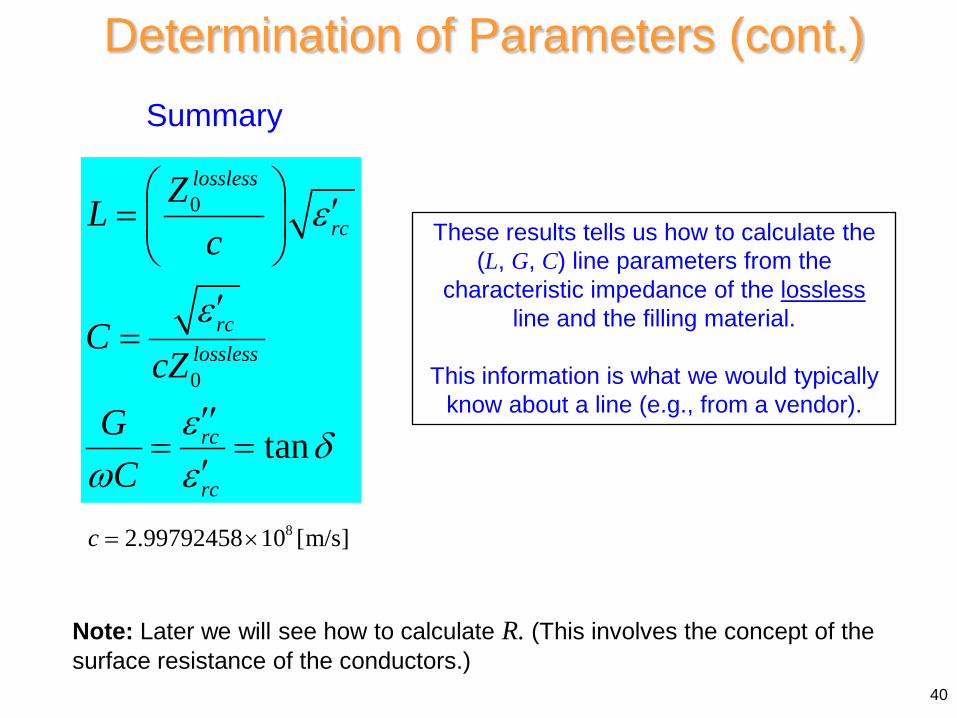
Determination of Parameters (cont.) Summary

0

0

tan

lossless

rc

rclossless

rc

rc

ZLc

CcZ

GC

ε

ε

ε δω ε

′=

′

=

′′= =

′

Note: Later we will see how to calculate R. (This involves the concept of the surface resistance of the conductors.)

These results tells us how to calculate the (L, G, C) line parameters from the

characteristic impedance of the lossless line and the filling material.

This information is what we would typically

know about a line (e.g., from a vendor).

82.99792458 10 [m/s]c = ×

40

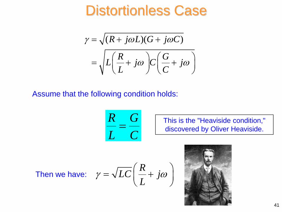
Distortionless Case

( )( )R j L G j C

R GL j C jL C

γ ω ω

ω ω

= + +

= + +

R GL C=

RLC jL

γ ω = +

Assume that the following condition holds:

Then we have:

This is the "Heaviside condition," discovered by Oliver Heaviside.

41

Distortionless Case (cont.)

1( )p

R LC LCL

vLC

α β ω

ω

= =

= = constant (no dispersion)

RLC jL

γ ω = +

There is then attenuation but no dispersion.

,G Rω ω∝ ∝

42

(assuming a fixed loss tangent) LR GC

=

Also, there will be distortion since α is a function of frequency.

Note: There will be some distortion in practice, since the Heaviside condition cannot be satisfied for all frequencies:


43

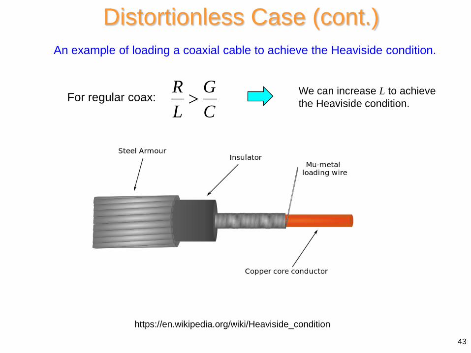
https://en.wikipedia.org/wiki/Heaviside_condition

An example of loading a coaxial cable to achieve the Heaviside condition.

R GL C> We can increase L to achieve

the Heaviside condition. For regular coax:


44

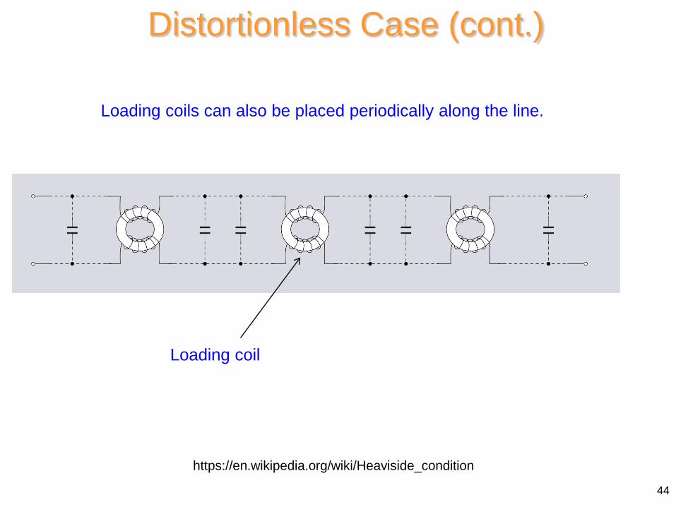
https://en.wikipedia.org/wiki/Heaviside_condition

Loading coils can also be placed periodically along the line.

Loading coil


45

Loading cables to improve performance was popular in the early 1900’s, but declined after the 1940s.

The technology has been superseded by using digital repeaters on transmission lines.

For long distances, transmission lines are usually replaced by fiber-optic cables (or wireless systems).

For an interesting history:

https://en.wikipedia.org/wiki/Loading_coil

ECE 6340 Intermediate EM Waves - University of Houstoncourses.egr.uh.edu/ECE/ECE6340/Class...

Documents

Transcript of ECE 6340 Intermediate EM Waves - University of Houstoncourses.egr.uh.edu/ECE/ECE6340/Class...