- 1 -

Do Credit Shocks Matter? A Global Perspective*

Thomas HelblingΥ Raju Huidromµ M. Ayhan KoseΥ Christopher Otrokµβ

July 2010 Abstract: This paper examines the importance of credit market shocks in driving global business cycles over the period 1988:1-2009:4. We estimate common components of various macroeconomic and financial variables of the G-7 countries. We then undertake a variety of exercises to evaluate the role played by credit market shocks using a global VAR model. Our findings suggest that these shocks do matter in explaining global business cycles. In particular, they have been influential in driving global activity during the 2009 global recession. We also study the global implications of credit market shocks originating in the U.S. We show that the U.S. credit market shocks have a significant impact on the evolution of global growth during the latest episode. Copyright Rests With Authors ______________________________ * We would like to thank David Fritz and Ezgi Ozturk for providing outstanding research assistance. The views expressed in this paper are those of the authors and do not necessarily represent those of the IMF or IMF policy. β Corresponding author Υ International Monetary Fund, Research Department; thelbling@imf.org (Helbling); akose@imf.org (Kose). µ University of Virginia, Department of Economics; rh2cw@virginia.edu (Huidrom); otrok@virginia.edu (Otrok)

- 2 -

I. Introduction

The global financial crisis of 2007-09 that originated in U.S. credit markets rapidly

spread across borders and led to recessions or severe downturns in almost all advanced

economies and many emerging economies at the same time. The global reach and depth

of the crisis, which are without precedent in the post-World War II period, have renewed

interest in the linkages between the real economy and credit markets and have triggered

an intensive debate about the importance of shocks originating in financial markets for

business cycles. Our objective in this paper is to attempt to answer one of the central

questions of this debate: Do credit shocks matter in the global economy?

We study this question by analyzing the importance of a fairly comprehensive set of

shocks in the context of G-7 countries. We estimate common components of various

macroeconomic and financial variables, and examine the roles played by credit shocks in

explaining global business cycles employing a set of VAR models. In addition, we study

the transmission of credit shocks in the U.S. to the global economy using a factor-

augmented VAR (FAVAR). Our results suggest that credit shocks play an important role

in the global recessions.

Our study contributes to a large body of research focusing on the interactions between

financial markets and the real economy. A short review of this literature reveals the

central nature of the question we are studying. Depending on the class of models under

consideration, the role of credit markets in driving business cycles varies substantially.

While some models consider that the credit markets are only peripherally important for

the dynamics of business cycles, some others assign a significant importance to the

shocks originating in credit markets.1

1 While the early literature did recognize that financial markets play an important role in the real economy, this emphasis later faded. Shocked by the experiences of the Great Depression, Fisher (1933) and Keynes were among the first to emphasize the importance of financial markets in shaping macroeconomic outcomes. Subsequent research, however, focused largely on the role of money as the most relevant financial variable to aggregate economic behaviors. The famous Modigliani and Miller (MM) (1958) “capital structure

(continued)

- 3 -

Basic economic theory suggests that, in a frictionless world under complete markets,

macroeconomic and financial variables can interact closely through wealth and

substitution effects. Developments in credit markets, which are simply reflected by

movements in asset prices, can influence consumption through their impact on household

wealth, and can affect investment by altering a firm’s net worth and the market value of

the capital stock relative to its replacement value (see Campbell, 2003; Cochrane, 2006).

However, in models with complete markets, the financial sector is a “veil” in the sense

that there is no role for financial intermediaries or credit market disturbances, since these

models do not consider financial imperfections/frictions. These models, hence, imply that

shocks originating in credit markets play only a minor role, if any, in explaining business

cycles.

In theory, interactions between financial variables and the real economy can be amplified

when financial imperfections are present.2 This amplification largely occurs through the

financial accelerator and related mechanisms operating through firms, households and

countries’ balance sheets. According to these mechanisms, an increase (decrease) in asset

prices improves an entity’s net worth, enhancing (reducing) its capacities to borrow,

invest and spend. This process, in turn, can lead to further increases (decreases) in asset

prices and have general equilibrium effects (e.g., Bernanke and Gertler, 1989; Bernanke,

Gertler, and Gilchrist, 1999; Kiyotaki and Moore, 1997; and numerous other studies on

the role of financial imperfections). In other words, disturbances in credit markets can

translate into much larger cyclical fluctuations in the real sector in these models.3

irrelevance” hypothesis and the general focus on efficient financial markets, however, may have inadvertently drawn attention away from the relevance of financial structure for macroeconomic performance.

2 Surveys of this literature can be found in Gertler (1988), Bernanke (1993), Lowe and Rohling (1993), and Bernanke, Gertler, and Gilchrist (1996), and Gilchrist and Zakrajsek (2010). 3 Some recent studies have focused on the role of asset prices as vehicles in transmitting financial cycles (Adrian and Shin, 2009; and Geanakoplos, 2009). Recent studies also consider how the state of the financial system can affect business cycles (Gertler and Kyotaki, 2010; Brunnermeier and Sannikov, 2010).

- 4 -

Other studies applying models of frictions in credit markets to open economies have

considered how the dynamics of another asset price, exchange rate, relate to business

cycles (see Cespedes, Chang and Velasco, 2004).4 This line of research also studies how

fluctuations in asset prices can affect the value of collateral required for international

funding (see Mendoza, 2010). Caballero and Krishnamurthy (1998) and Schneider and

Tornell (2004) model how, because of balance sheet constraints, fluctuations in credit and

asset markets translate into boom-bust cycles in emerging market economies.5

Many empirical studies provide evidence regarding the linkages between the dynamics of

business cycles and disturbances in credit markets (e.g., Bernanke and Gertler, 1989;

Borio, Furfine and Lowe, 2001). Many of these examine the procyclical nature of credit

cycles and business fluctuations, albeit mostly for single country cases. For example,

Bordo and Haubrich (2010) analyze cycles in money, credit and output between 1875 and

2007 in the United States. They show that financial stress events exacerbate cyclical

downturns. While most studies have used aggregate data, some credit-related studies

have been based on micro data (banks or corporations).6

Our paper is closely related to some recent studies analyzing the importance of credit

shocks using VAR models. Meeks (2009) examines the importance of credit shocks in

explaining U.S. business cycles. He documents that credit shocks do play an important

role during financial crises, but they have a lesser role during normal business cycles.

Gilchrist, Yankov and Zakrajsek (2009) and Gilchrist and Zakrajek (2010) report that

credit market spreads have a significant impact on business cycles in the U.S. during the

period 1990-2008.

4 Earlier work includes Krugman (1999) and Aghion, Bacchetta and Banerjee (2000). 5 There is also a rich set of theoretical studies analyzing the implications of various types of financial crises for the real economy (see Gorton, 2009 as regard to the recent financial crisis). 6 See Bernanke, Gertler and Gilchrist, 1996; Kashyap and Stein, 2000; and Kannan, 2010.

- 5 -

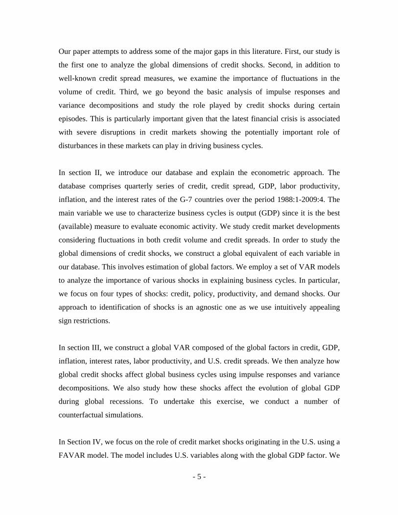
Our paper attempts to address some of the major gaps in this literature. First, our study is

the first one to analyze the global dimensions of credit shocks. Second, in addition to

well-known credit spread measures, we examine the importance of fluctuations in the

volume of credit. Third, we go beyond the basic analysis of impulse responses and

variance decompositions and study the role played by credit shocks during certain

episodes. This is particularly important given that the latest financial crisis is associated

with severe disruptions in credit markets showing the potentially important role of

disturbances in these markets can play in driving business cycles.

In section II, we introduce our database and explain the econometric approach. The

database comprises quarterly series of credit, credit spread, GDP, labor productivity,

inflation, and the interest rates of the G-7 countries over the period 1988:1-2009:4. The

main variable we use to characterize business cycles is output (GDP) since it is the best

(available) measure to evaluate economic activity. We study credit market developments

considering fluctuations in both credit volume and credit spreads. In order to study the

global dimensions of credit shocks, we construct a global equivalent of each variable in

our database. This involves estimation of global factors. We employ a set of VAR models

to analyze the importance of various shocks in explaining business cycles. In particular,

we focus on four types of shocks: credit, policy, productivity, and demand shocks. Our

approach to identification of shocks is an agnostic one as we use intuitively appealing

sign restrictions.

In section III, we construct a global VAR composed of the global factors in credit, GDP,

inflation, interest rates, labor productivity, and U.S. credit spreads. We then analyze how

global credit shocks affect global business cycles using impulse responses and variance

decompositions. We also study how these shocks affect the evolution of global GDP

during global recessions. To undertake this exercise, we conduct a number of

counterfactual simulations.

In Section IV, we focus on the role of credit market shocks originating in the U.S. using a

FAVAR model. The model includes U.S. variables along with the global GDP factor. We

- 6 -

study how the credit shocks affect U.S. macroeconomic aggregates. In addition, we

analyze how these shocks are transmitted to the global economy considering their impact

on global GDP. We conclude in Section V with a brief summary of our main results and

directions for future research.

II. Database and Methodology

II.1. Database

Our dataset includes quarterly series of credit, credit spread, GDP, labor productivity,

inflation, and the interest rates of the G-7 countries during the period 1988:1-2009:4. We

are interested in this period because of the following reasons. First, it is a common

denominator for the cross-country data we need to analyze the interaction between credit

shocks and business cycle dynamics in the G-7 countries. Second, this period covers a

substantial portion of the era of the so-called “Great Moderation” as well as the latest

global financial crisis.7 Third, this period also coincides with a rapid increase in trade and

financial linkages across these countries and overlaps with a broader converge of their

business cycles (see Kose, Otrok, and Whiteman, 2008).8

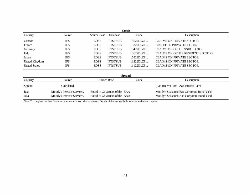
Our measure of credit is aggregate claims on the private sector by deposit money banks.

This measure is also used in earlier cross-country studies on credit dynamics (see

Mendoza and Terrones, 2008 and Claessens, Kose, and Terrones, 2009 and 2010). The

use of credit volume differentiates our study from most others analyzing the impact of

credit shocks and allows us to construct a global credit factor since this variable is

7 The era of Great Moderation started in the mid-1980s and coincided with a structural decline in the volatility of business cycles in industrial countries until the financial crisis of 2008-09. For details about the Great Moderation, see Blanchard and Simon (2001), McConnell and Perez-Quiros (2000) and Stock and Watson (2005). 8 In particular, using a dynamic factor model, Kose, Otrok and Whiteman (2008) find that that the degree of comovement of business cycles in major macroeconomic aggregates across the G-7 countries has increased during the globalization period starting in the mid-1980s.

- 7 -

available for all of the G-7 countries at the quarterly frequency.9

We deflate the nominal

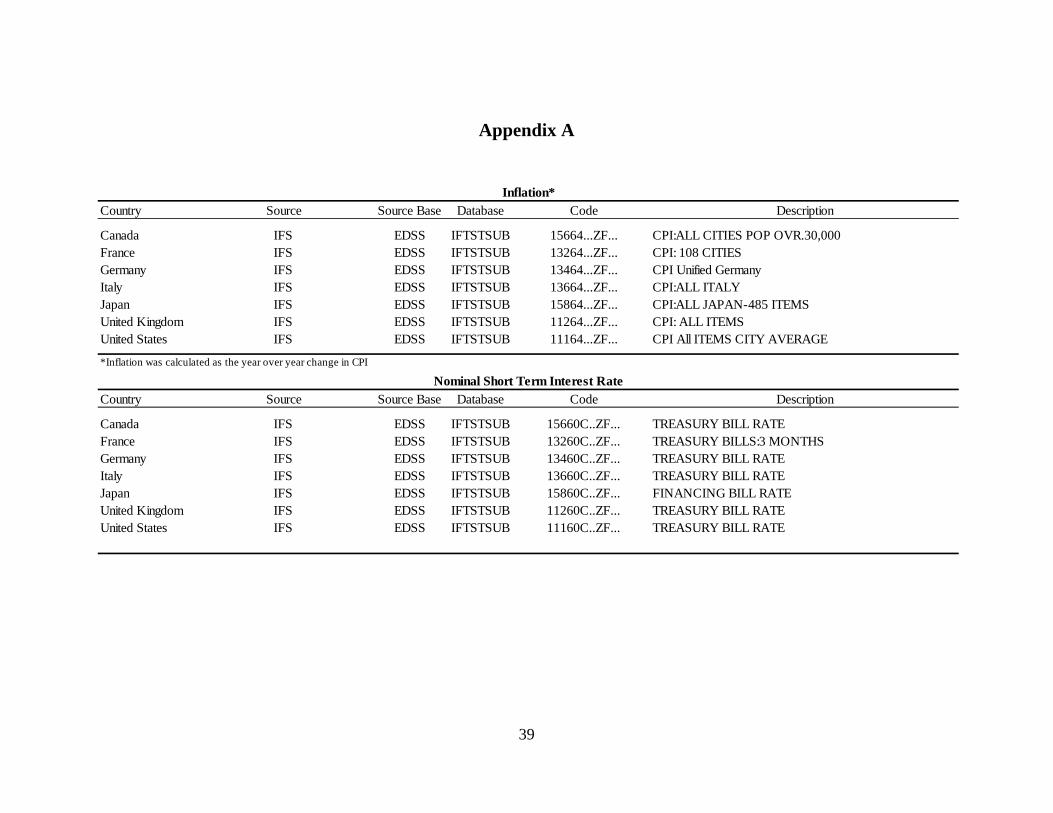
credit series using the CPI to produce real credit. Inflation corresponds to the changes in

each country’s CPI. Both credit and CPI series are from the International Financial

Statistics (IFS).

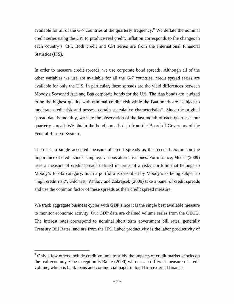
In order to measure credit spreads, we use corporate bond spreads. Although all of the

other variables we use are available for all the G-7 countries, credit spread series are

available for only the U.S. In particular, these spreads are the yield differences between

Moody's Seasoned Aaa and Baa corporate bonds for the U.S. The Aaa bonds are “judged

to be the highest quality with minimal credit” risk while the Baa bonds are “subject to

moderate credit risk and possess certain speculative characteristics”. Since the original

spread data is monthly, we take the observation of the last month of each quarter as our

quarterly spread. We obtain the bond spreads data from the Board of Governors of the

Federal Reserve System.

There is no single accepted measure of credit spreads as the recent literature on the

importance of credit shocks employs various alternative ones. For instance, Meeks (2009)

uses a measure of credit spreads defined in terms of a risky portfolio that belongs to

Moody’s B1/B2 category. Such a portfolio is described by Moody’s as being subject to

“high credit risk”. Gilchrist, Yankov and Zakrajsek (2009) take a panel of credit spreads

and use the common factor of these spreads as their credit spread measure.

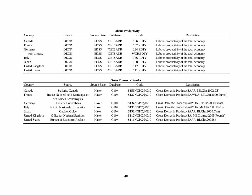
We track aggregate business cycles with GDP since it is the single best available measure

to monitor economic activity. Our GDP data are chained volume series from the OECD.

The interest rates correspond to nominal short term government bill rates, generally

Treasury Bill Rates, and are from the IFS. Labor productivity is the labor productivity of

9 Only a few others include credit volume to study the impacts of credit market shocks on the real economy. One exception is Balke (2000) who uses a different measure of credit volume, which is bank loans and commercial paper in total firm external finance.

- 8 -

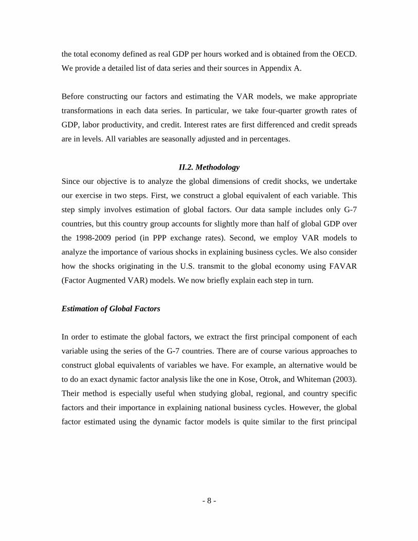
the total economy defined as real GDP per hours worked and is obtained from the OECD.

We provide a detailed list of data series and their sources in Appendix A.

Before constructing our factors and estimating the VAR models, we make appropriate

transformations in each data series. In particular, we take four-quarter growth rates of

GDP, labor productivity, and credit. Interest rates are first differenced and credit spreads

are in levels. All variables are seasonally adjusted and in percentages.

II.2. Methodology

Since our objective is to analyze the global dimensions of credit shocks, we undertake

our exercise in two steps. First, we construct a global equivalent of each variable. This

step simply involves estimation of global factors. Our data sample includes only G-7

countries, but this country group accounts for slightly more than half of global GDP over

the 1998-2009 period (in PPP exchange rates). Second, we employ VAR models to

analyze the importance of various shocks in explaining business cycles. We also consider

how the shocks originating in the U.S. transmit to the global economy using FAVAR

(Factor Augmented VAR) models. We now briefly explain each step in turn.

Estimation of Global Factors

In order to estimate the global factors, we extract the first principal component of each

variable using the series of the G-7 countries. There are of course various approaches to

construct global equivalents of variables we have. For example, an alternative would be

to do an exact dynamic factor analysis like the one in Kose, Otrok, and Whiteman (2003).

Their method is especially useful when studying global, regional, and country specific

factors and their importance in explaining national business cycles. However, the global

factor estimated using the dynamic factor models is quite similar to the first principal

- 9 -

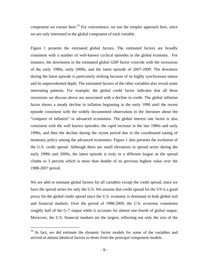
component we extract here.10

For convenience, we use the simpler approach here, since

we are only interested in the global component of each variable.

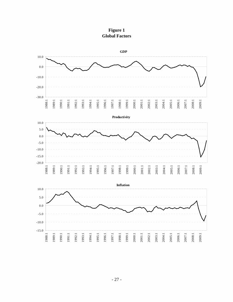
Figure 1 presents the estimated global factors. The estimated factors are broadly

consistent with a number of well-known cyclical episodes in the global economy. For

instance, the downturns in the estimated global GDP factor coincide with the recessions

of the early 1990s, early 2000s, and the latest episode of 2007-2009. The downturn

during the latest episode is particularly striking because of its highly synchronous nature

and its unprecedented depth. The estimated factors of the other variables also reveal some

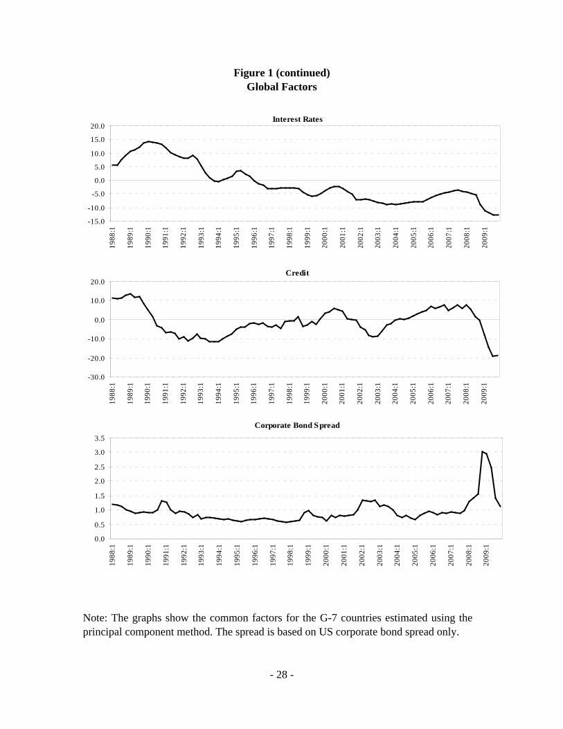
interesting patterns. For example, the global credit factor indicates that all three

recessions we discuss above are associated with a decline in credit. The global inflation

factor shows a steady decline in inflation beginning in the early 1990 until the recent

episode consistent with the widely documented observation in the literature about the

“conquest of inflation” in advanced economies. The global interest rate factor is also

consistent with the well known episodes: the rapid increase in the late 1980s and early

1990s, and then the decline during the recent period due to the coordinated easing of

monetary policy among the advanced economies. Figure 1 also presents the evolution of

the U.S. credit spread. Although there are small elevations in spread series during the

early 1990s and 2000s, the latest episode is truly in a different league as the spread

climbs to 3 percent which is more than double of its previous highest value over the

1988-2007 period.

We are able to estimate global factors for all variables except the credit spread, since we

have the spread series for only the U.S. We assume that credit spread for the US is a good

proxy for the global credit spread since the U.S. economy is dominant in both global real

and financial markets. Over the period of 1988-2009, the U.S. economy constitutes

roughly half of the G-7 output while it accounts for almost one-fourth of global output.

Moreover, the U.S. financial markets are the largest, reflecting not only the size of the

10 In fact, we did estimate the dynamic factor models for some of the variables and arrived at almost identical factors to those from the principal component models.

- 10 -

economy but also their depth. For example, capitalization of the U.S. equity markets

accounts for around 40 percent of total capitalization of world equity markets. Changes in

U.S. credit markets and asset prices have strong signaling effects worldwide, and

spillovers from U.S. financial markets have been important, especially during periods of

market stress.

VAR Models

We estimate two VAR models. The first one is a “global” VAR model including the

estimated global factor of each variable and the U.S. credit spread. The second model is a

FAVAR as it uses the U.S. specific variables along with the global GDP factor.11

Yt = A(0) + A(1)Y(t−1) + A(2)Yt−2 + … . + A(l)Yt−l + ut ; t = 1, … , T

The

models we have can be represented by:

where Yt is an m × 1 vector of variables at date t, Ai is an m × m coefficient matrix for

each lag of the variable vector with A(0) being the constant term. ut is the vector of one-

step ahead prediction error. The global VAR and the U.S. FAVAR differ only in terms of

the set of variables in the Yt vector. For the global VAR, Yt includes the estimated global

factors and U.S. credit (i.e., corporate bond) spread.12

In the case of the U.S. FAVAR, the

vector consists of the set of U.S. variables and the global GDP factor. In our estimation,

the lag length, 𝑙, is kept at four.

We use these models to examine the roles of four shocks in explaining the global and

U.S. business cycles: credit, policy, productivity, and demand shocks. In addition to

11 Our model follows the work of Bernanke, Bovin, and Eliasz (2005) who developed the factor-augmented VAR (FAVAR) to study the effects of monetary policy in a closed economy framework. 12 Bernanke, Bovin, and Eliasz (2005) compare FAVARs that treat estimated factors as data as is done here, with more sophisticated Bayesian estimates that account for uncertainty in the estimated factors. They find that there is no real gain from the more computationally intensive Bayesian methods for this type of problem.

- 11 -

credit market shocks, we focus on the shocks stemming from changes in policies,

productivity, and demand since different classes of models emphasize their importance in

explaining business cycles. We use global and the U.S. specific versions of these shocks

in our respective models of the global economy and the U.S.

We identify the shocks using the idea of sign restrictions imposed on impulse responses

following Uhlig (2005).13

Instead of relying on informational orderings about the

importance of shocks, this identification approach allows us to produce impulse

responses that are qualitatively consistent with the standard theoretical predictions. The

sign restrictions we impose are indeed intuitively appealing. For example, we identify

adverse credit market shocks as those that correspond to a decrease in credit and an

increase in credit spreads for four quarters following the initial shock. While this

identification scheme describes the natural responses of volume and price of credit to

disturbances in credit markets, it does not impose any restriction on the response of GDP.

Analogously, our contractionary policy shocks are identified by assuming that they are

associated with an increase in the interest rates, a fall in GDP, a fall in inflation, and a fall

in credit spreads. The fall in credit spreads, the last restriction we impose to identify

policy shocks, purges these shocks from credit shocks. To identify positive demand

shocks, we consider these shocks coinciding with an increase in both GDP and inflation.

Lastly, the identification of a positive productivity shock implies that such a shock

corresponds to an increase in labor productivity, an increase in GDP, and a fall in

inflation. The latter restriction on inflation can be formally derived from a New

Keynesian DSGE model. In that model inflation is driven by marginal cost, and positive

productivity shocks lower marginal cost.

13 Uhlig (2005) employs this method in a different context as he considers the importance of monetary policy shocks by imposing sign restrictions on the impulse responses of prices, nonborrowed reserves and the federal funds rate in response to a monetary policy shock.

- 12 -

We keep the horizon for sign restrictions for all of the shocks at four quarters to maintain

symmetry across different shocks. The horizon of four quarters also captures the idea that

each shock persists for at least a year.14

We conduct sensitivity exercises to check the

robustness of our results to alternative identification restrictions and their durations and

all of our main results are robust to these variations.

III. Credit Shocks and Global Business Cycles

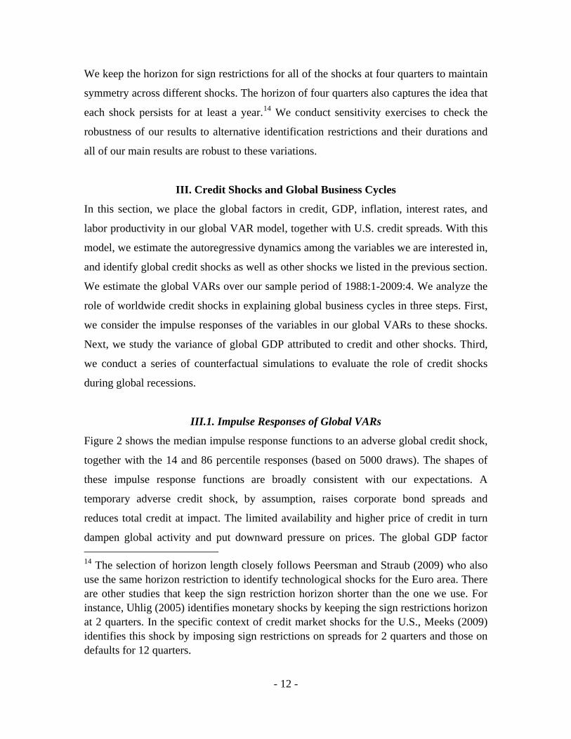
In this section, we place the global factors in credit, GDP, inflation, interest rates, and

labor productivity in our global VAR model, together with U.S. credit spreads. With this

model, we estimate the autoregressive dynamics among the variables we are interested in,

and identify global credit shocks as well as other shocks we listed in the previous section.

We estimate the global VARs over our sample period of 1988:1-2009:4. We analyze the

role of worldwide credit shocks in explaining global business cycles in three steps. First,

we consider the impulse responses of the variables in our global VARs to these shocks.

Next, we study the variance of global GDP attributed to credit and other shocks. Third,

we conduct a series of counterfactual simulations to evaluate the role of credit shocks

during global recessions.

III.1. Impulse Responses of Global VARs

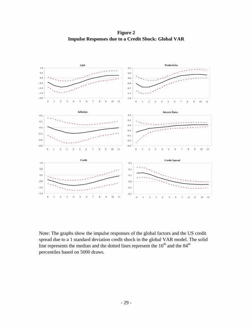
Figure 2 shows the median impulse response functions to an adverse global credit shock,

together with the 14 and 86 percentile responses (based on 5000 draws). The shapes of

these impulse response functions are broadly consistent with our expectations. A

temporary adverse credit shock, by assumption, raises corporate bond spreads and

reduces total credit at impact. The limited availability and higher price of credit in turn

dampen global activity and put downward pressure on prices. The global GDP factor 14 The selection of horizon length closely follows Peersman and Straub (2009) who also use the same horizon restriction to identify technological shocks for the Euro area. There are other studies that keep the sign restriction horizon shorter than the one we use. For instance, Uhlig (2005) identifies monetary shocks by keeping the sign restrictions horizon at 2 quarters. In the specific context of credit market shocks for the U.S., Meeks (2009) identifies this shock by imposing sign restrictions on spreads for 2 quarters and those on defaults for 12 quarters.

- 13 -

declines at impact, as does the global inflation. Short-term interest rates fall as well,

presumably reflecting monetary easing in response to an unexpected tightening in credit

markets. This is reassuring because it suggests that with our identification assumption, we

do not capture monetary policy-induced credit tightening. The dampening effects of a

credit shock gradually intensify over 2 quarters for real-sector variables (GDP and labor

productivity) and over 4 quarters for nominal variables (inflation and interest rates)

before they fade gradually.

The direct impact of credit shocks on the key variables capturing the credit channel, the

global credit factor and the spreads, which serve to identify the credit shocks, are

statistically significant. Beyond the direct credit market effects, the transmission of these

shocks to other variables also conforms to conventional wisdom, but the dynamic effects

are not always statistically significant. Importantly, however, the output effects are

significant.15

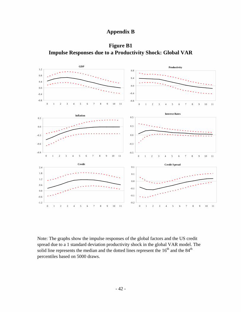
We present the responses to other global shocks in Figures B1-B3 in Appendix B. As in

the case of credit shocks, the impulses due to policy, productivity, and demand shocks

generally have the expected patterns in terms of signs. However, they are not statistically

significant except for the initial four quarters imposed for identification. In particular, our

results suggest the responses of credit variables to other shocks are not always significant

and often surprisingly muted. This aspect of our findings highlights that the transmission

of shocks through credit channels may not always be relevant.

We also analyze the robustness of our results with respect to different identification

schemes. Specifically, we identify credit shocks by selecting only impulse responses with

either a positive credit spread response or a negative credit growth response. The results

are virtually identical to those obtained with our baseline identification scheme.16

15 The significance of impulse responses of spreads and credit is valid only during the initial 4 quarters where we restrict them a priori to identify credit shocks.

16 These results are available from the authors upon request.

- 14 -

III.2. Variance Decompositions of Global VARs

The insignificance of the responses of global real and nominal variables to credit shocks

does not necessarily imply that these shocks are not important. In fact, our variance

decompositions suggest that measured by their contribution to fluctuations to the global

GDP factor, credit shocks are as important as other shocks. We report our findings in

Table 1. The reported variance decompositions are not based on a set of orthogonal

shocks that add up to 100 percent. Instead, they reflect a sequence of variance

decompositions, each one for one structural shock at a time (with the shocks identified as

discussed above). In other words, each cell refers to the contribution of the respective

shock to the variance of a particular variable while the rest of the variance is accounted

by all other potential unidentified shocks.

The credit shock, for example, accounts for roughly 14 percent of the 12-quarter ahead

forecast error variance of the global GDP factor, implying that a universe of other,

orthogonal but unidentified, shocks account for the rest. Consequently, the fact that our

plain vanilla demand shock accounts for 10 percent as well does not imply that the

contributions of credit and demand shocks together add up to 25 percent, as they would in

a standard decomposition. Instead, our decompositions suggest that credit shocks account

for about as large a share of fluctuations on their own as other, standard structural

macroeconomic shocks. Productivity and policy shocks account for approximately 13 and

12 percent of variation in global GDP, respectively.

In addition to global GDP, credit shocks play an important role in explaining the variance

of other variables. For example, these shocks explain almost 13 percent of the variance of

global productivity. They account for around 15-16 percent of variation in inflation and

interest rates. We have so far focused on the importance of credit shocks over the period

1988-2009. We now turn to a different exercise and consider how these shocks affect

global GDP during certain episodes.

III.3. Credit Shocks during Global Recessions

- 15 -

How important are global credit shocks during episodes of global recessions? This is an

obvious question to ask given that the latest episode is a global event associated with

serious problems in global credit markets. We also consider the roles played by credit

shocks during the global recession of 1990-1991. These two episodes of global recessions

correspond to declines in world real GDP per capita.17

While the Great Recession of

2007-2009 is associated mainly with financial sector problems, the previous global

recession reflects a host of issues in various corners of the world: difficulties in the U.S.

saving and loan industry, banking crises in several Scandinavian economies, adverse

effects of an exchange rate crisis on a large number of European countries, challenges

faced by the east European transition economies, and the uncertainty stemming from the

Gulf War.

To gauge the role of credit shocks during these episodes, we perform a number of

counterfactual exercises. Each of these counterfactual exercises represents simulations

where the structural shock of interest is set to zero over the relevant period. In the case of

the latest episode, for example, the counterfactual credit shock simulation shows how the

global GDP factor would have evolved without the adverse “credit event” that has been

the hallmark of the Great Recession. It is important to recognize that this exercise sets the

shock itself to zero, but that does not imply that, say, the volume of credit does not

contract. Other shocks may also affect credit, and credit may respond endogenously to

other variables such as output through the lag structure of the VAR. What we are

eliminating then, is the unforecastable shock that drove up credit spreads and lower credit

volume.

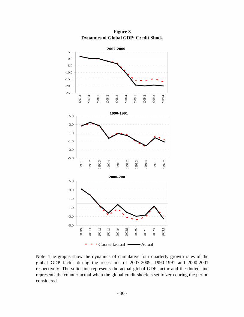
The top panel in Figure 3 compares the results of counterfactual simulations for the

global GDP factor during the Great Recession episode. Specifically, it shows the

differences between the actual cumulative change in the demeaned global GDP factor and

17 Our definition of global recessions follows Kose, Loungani, and Terrones (2010). In particular, they identify four troughs in global economic activity over the past 50 years—1975, 1982, 1991, and 2009.

- 16 -

the cumulative changes in the simulated values in the absence of the global credit shock

over the 2007:3-2009:4 period. It is obvious that the impact of the global credit shock has

become more pronounced as the recession has translated into a global event spreading

from the U.S. to other advanced countries. For example, without the credit shock, the

global recession would have been about 25 percent milder based on the differences

between the actual and simulated cumulative growth numbers in 2009:3.

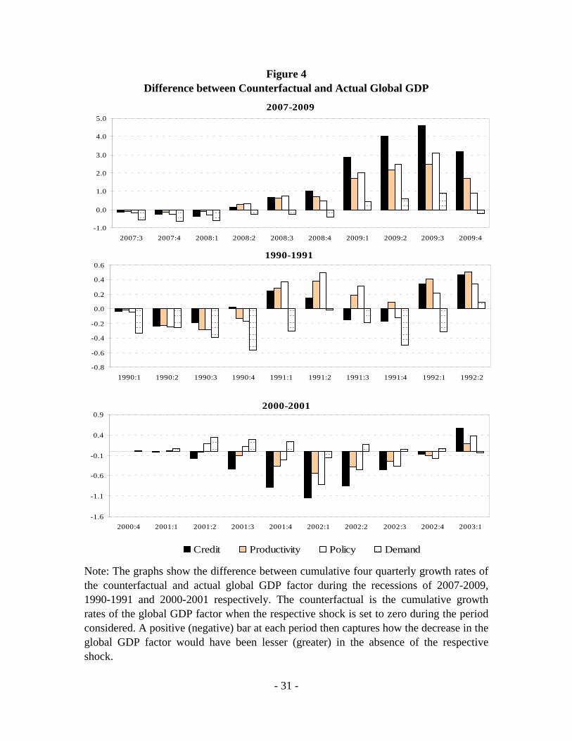
Figure 4 presents the contribution of each shock to the cumulative global GDP growth

based on counterfactual exercises. Comparing the counterfactual simulations across

shocks suggests that credit shocks on their own account for a larger share of the

cumulative change in the global GDP factor than the other shocks. We interpret this

result as evidence for the important role of credit shocks in the Great Recession.

Counterfactual simulations for the 1990-1991 global recession suggests, however, that

credit shocks have not always played the important role as they have done in the most

recent downturn. This can be seen in the middle panel of Figures 3 and 4, which show the

results from counterfactual simulations for that episode. These results suggest that while

credit shocks appear to have played some role in the 1991 downturn, their role is less

stark than it is in the 2008-2009 downturn. This finding is an intuitively appealing one.

As we discuss above, unlike the 2007-2009 episode which is mainly driven by difficulties

in credit markets, the 1990-1991 global recession stems from a variety of problems. As

we show in the next section, the impact of credit shocks is quite sizeable during the 1990-

1991 episode in the U.S. where credit markets went through a prolonged period of

contraction. Moreover, the latest episode is a truly synchronized one as both real and

financial sectors of the G-7 countries simultaneously experience major disruptions.18

18 Imbs (2010), using monthly data on industrial production, concludes that the degree of cross-country business cycle correlations during the latest crisis was the highest in three decades.

- 17 -

In addition to the global recessions of 1991 and 2009, we consider the downturn in global

growth in 2001 where a number of advanced countries experience much milder

recessions.19

This episode is associated with the bursting of “dot-com” equity bubbles in a

number of advanced countries following the rapid acceleration of stock prices of IT

companies during 1995-2000. We present the results for the 2001 episode in the bottom

panels of Figures 3 and 4. Given the equity market related nature of the 2001 episode

along with its milder effect on global GDP, credit shocks appear to have played a

somewhat stabilizing, albeit minimal, role. Hence, the decline in the global credit factor

would have been an endogenous response to the downturn in activity (and problems in

other segments of the financial sector, especially equity markets).

The conclusions we draw from the analysis in this section is that credit shocks matter for

the global economy, albeit to varying degrees. Their effects may not generally be large,

but credit shocks have played an important role in some episodes, notably during the

latest global recession. Such ambiguities in the effects of credit shocks are not new. Other

studies analyzing the relationship between financial conditions and future economic

activity and inflation at the country level have also often found weak and unstable

predictive power.20

19 According to Kose, Loungani, and Terrones (2010), the year 2001 does not get identified as a global recession since world real GDP per capita did not decline. Although many advanced countries had recessions, growth in major emerging markets such as China and India remained robust during that period.

One notable exception is that of Gilchrist, Yankov and Zakrajsek

(2009) who argue that the predictive power of credit spreads for economic activity

20 There is a large literature analyzing the predictive power of financial variables for future activity. However, the predictive value of these financial variables, including asset prices, generally is limited. Indeed, in their review, Stock and Watson (2003) conclude: “Some asset prices have been useful predictors of inflation and/or output growth in some countries in some periods.” In addition, the leading indicator property of asset price changes appears to be limited to certain classes of assets and dependent on the depth of asset markets in the different countries. A number of studies have documented the predictive value of interest rates for output fluctuations and the timing of recessions and recoveries. Specifically, the slope of the yield curve or the term spread—the difference between the long and the short-term interest rate—has long been recognized to have significant predictive power (see Wheelock and Wohar, 2009 for a recent review).

- 18 -

increases substantially, especially at longer horizons, when the measure of credit spreads

is derived from securities issued by intermediate-risk rather than high-risk firms.

IV. The Global Transmission of U.S. Credit Shocks

We have so far considered the role played by global credit shocks in explaining global

GDP. There is much to be said about rapidly increasing international financial linkages,

which have led to the speedy transmission of domestic credit shocks to other economies.

National and global credit shocks may thus have partly become indistinguishable.

Nevertheless, in view of the key role of the U.S. financial system in global financial

markets and the large size of the U.S. economy, a key question is whether credit shocks

that originate in the U.S. have international repercussions. In this section, we examine

this question by analyzing a set of FAVAR models with U.S. variables along with the

global GDP factor estimated earlier. As in the previous section, we consider the role of

U.S. credit shocks by first studying impulse responses, then variance decompositions, and

finally global recession episodes.

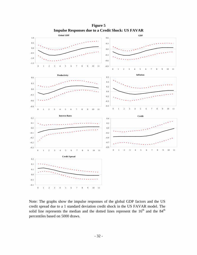
The impulse response functions to a U.S. credit shock are shown in Figure 5. The shapes

of the median responses are broadly similar to those of the global VAR in the previous

section, but there also are some differences. In particular, the impact effects of a 1

standard deviation credit shock on most of the variables are more modest than those in

the case of the global VAR. A major feature of the effects of a U.S. credit shock is that it

has noticeable international repercussions. In response to such a shock, the global GDP

factor declines, with patterns that are broadly similar to those found for the U.S. GDP. As

in the case of the effects of global credit shocks, however, the dynamic effects generally

are statistically significant for activity but not inflation and nominal interest rates.21

21 As in the case of the global VAR, we also identify other structural U.S. specific shocks using the identification schemes described in section II. The impulse responses to these shocks are presented in Figures B4 to B6 in Appendix B. The findings are broadly consistent with the ones from the global VARs.

- 19 -

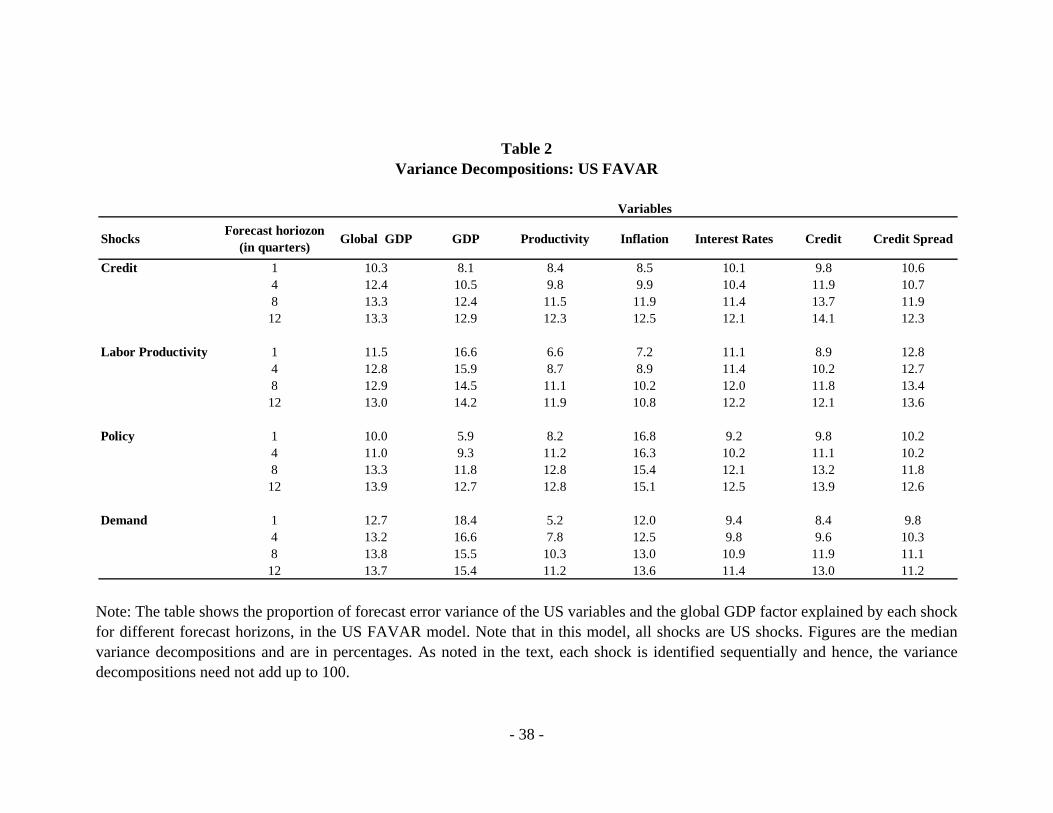
Table 2 presents our findings with respect to the variance decompositions. U.S. credit

shocks play an important role in explaining the variance of domestic macroeconomic

aggregates. For example, they account for 13 percent of fluctuations in the U.S. GDP

(based on the 12 quarters ahead forecast error variance). Our estimate of the fraction of

variance of the U.S. GDP due to a credit shock is consistent with the findings by Meeks

(2009).22

More interestingly, the U.S. credit shocks account for 13 percent of the variance

of global GDP confirming the important role played by the disturbances in the U.S. credit

markets for the global economy.

We also compute variance decompositions for other structural U.S. specific shocks along

the lines described in section II. Comparing across shocks, the proportion of the 12-

quarter ahead forecast error variance explained by each shock fluctuates around a

uniform 13 percent. This reiterates our earlier point that credit shocks are as important as

other macroeconomic shocks in explaining business cycle fluctuations.

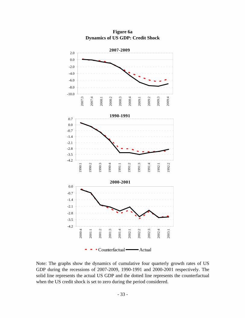
How important are U.S. credit shocks during global recessions? To answer this question,

we conduct a set of counterfactual exercises as in the previous section. Figure 6a (Figure

6b)shows the differences between the actual cumulative change in the demeaned U.S.

GDP (global GDP factor) and the cumulative changes in the simulated values of the same

variables in the absence of the U.S. credit shock during the three episodes we identify in

the previous section. Figures 7a-7b displays the differences between the actual and

counterfactual simulations for all the shocks.

Three major findings stand out from these figures. First, credit shocks again account for

the largest difference in the cumulative GDP change during the latest episode in the

counterfactual simulations, both for the U.S. GDP and the global GDP factor. This

22 The variance decompositions based on shocks, which are identified with sign restrictions, are generally different from those based on the standard recursive decompositions. We, thus, restrict comparison of our results against those studies utilizing sign restrictions only (see Meeks (2009) for a similar point).

- 20 -

finding corroborates our earlier results and current views about the main driving force

behind the latest episode.

The important role played by credit market disturbances in explaining the severity of

recessions during certain episodes is also consistent with some recent studies. For

example, Claessens, Kose, and Terrones (2009, 2010) analyze the interactions between

recessions and disruptions in credit and asset markets using a sample of 122 recessions in

21 advanced countries. Their findings suggest that when recessions coincide with a

substantial decline in credit, they tend to become deeper.

Second, the 1991 downturn in the U.S. was associated with adverse disturbances in the

credit markets, but not necessarily elsewhere. This conclusion follows from two facts. On

the one hand, U.S. credit shocks account for the largest difference between actual and

counterfactual simulations in the case of U.S. GDP, but not in the case of global GDP. On

the other hand, our earlier counterfactual simulations with the global VAR have already

shown that credit shocks generally do not account for the largest differences between

actual and counterfactual global GDP in the 1991 episode. This suggests that not all U.S.

credit shocks need to have strong global repercussions. Indeed, the 1991 credit shock in

the U.S. is widely seen as having had a strongly local component, as it primarily involved

financial institutions that were not internationally integrated. Specifically, the 1991

episode is associated with problems in the savings-and-loan industry in the United States.

Third, the U.S. FAVAR models confirm that the 2001 global downturn was not an

adverse credit event. Both the 1991 and 2009 global recessions coincided with financial

crises. However, as noted above, the 2001 episode, unlike the 1991 and 2009 global

recessions, is associated with disruptions in equity markets while the credit market was

only responding to contraction in activity. Indeed, our findings confirm that U.S. based

credit market disturbances did not appear to have played a meaningful role in explaining

variations in either U.S. GDP or the global GDP factor in this episode. Our results are

also consistent with those reported by Claessens, Kose, and Terrones (2009, 2010) who

- 21 -

find that recessions associated with equity price busts are not deeper than other

recessions.

V. Conclusion

The latest financial crisis has been a bitter reminder of the important role played by credit

markets in driving macroeconomic fluctuations. Although there has been a large research

program analyzing how gyrations in credit markets translate into fluctuations in the real

sector at the country level, the global dimensions of this issue have not yet been studied.

Our paper aims to provide a perspective about the linkages between credit markets and

global business cycles fluctuations using a simple framework. In particular, we analyze

the importance of credit market shocks for the G-7 countries using a global VAR model.

We start with a set of impulse responses to get a grasp of the dynamic reactions to

disturbances in credit markets. We find that these disturbances have a significant impact

on output, but their effects on other variables are not always substantial. We then conduct

variance decompositions to analyze how important the credit market shocks in driving

output fluctuations. The results of this exercise suggest that these shocks are as important

as other potential shocks, including productivity, demand, and policy shocks.

We then assess the role of credit shocks during global recessions. In particular, we

undertake a series of counterfactual exercises to examine the evolution of global GDP

during the 1991 and 2009 global recessions. We find that credit shocks have played an

important role during the latest global recession. Our simulations indicate that the impact

of credit shocks during the 1991 global recession is smaller, but this is mostly due to the

U.S. specific nature of the credit shock and the confluence of other factors during this

episode.

We also study the global implications of credit shocks that originate in the U.S. by

employing a set of FAVAR models. Our results with respect to the impulse responses and

variance decompositions of these models are mostly consistent with the ones from the

global VAR models. During the latest episode, U.S. credit shocks have been influential in

- 22 -

driving global growth dynamics. Moreover, they have played a major role in shaping the

evolution of U.S. business cycles during the 1991 recession. However, consistent with

our earlier findings, the impact of these shocks on global activity was minor during the

1991 episode.

We plan to extend our study in future work by considering the potential importance of

cross-country spillovers through various financial market linkages. In addition to credit

markets, it would be interesting to analyze how asset (equity and real estate) market

linkages can transmit business cycles across countries. In addition, it would be useful to

study the importance of credit market shocks originating in advanced countries for

emerging market economies.

- 23 -

References

Adrian, Tobias, and Hyun Song Shin, 2009, “Prices and Quantities in the Monetary Policy Transmission Mechanism,” International Journal of Central Banking, International Journal of Central Banking, Vol.5(4), pp. 131-142, December.

Aghion, Philippe, Philippe Bacchetta , and Abhijit Banerjee, 2000, “Currency Crises and Monetary Policy in an Economy with Credit Constraints,” Working Papers, No. 00-07, Swiss National Bank, Study Center Gerzensee.

Balke, Nathan S., 2000, “Credit and Economic Activity: Credit Regimes and Nonlinear Propagation of Shocks,” The Review of Economics and Statistics, Vol.82, No.2, pp.344-349.

Bernanke, Ben and Mark Gertler, 1989, “Agency Costs, Net Worth, and Business Fluctuations,” American Economic Review, Vol. 79, pp.14-31.

Bernanke, Ben S., 1993, “How important is the credit channel in the transmission of monetary policy? : A comment,” Carnegie-Rochester Conference Series on Public Policy, Elsevier, Vol. 39(1), pp. 47-52, December.

Bernanke, Ben, Jean Boivin, and Piotr S. Eliasz, 2005, “Measuring the Effects of Monetary Policy: A Factor-augmented Vector Autoregressive (FAVAR) Approach,” The Quarterly Journal of Economics, MIT Press, Vol. 120(1), pp. 387-422, January.

Bernanke, Ben, Mark Gertler, and Simon Gilchrist, 1996, “The Financial Accelerator and the Flight to Quality,” The Review of Economics and Statistics, Vol. 78, No. 1, (Feb.), 1-15.

Bernanke, Ben, Mark Gertler, and Simon Gilchrist,1999, "The Financial Accelerator in a Quantitative Business Cycle Framework," in Handbook of Macroeconomics, Vol. 1C, Handbooks in Economics, Vol. 15. Amsterdam: Elsevier, pp. 1341-1393.

Blanchard, Olivier, and John Simon, 2001, “The Long and Large Decline in U.S. Output Volatility,” Brookings Papers on Economic Activity, Economic Studies Program, The Brookings Institution,Vol. 32(2001-1), pp.135-174.

Bordo, Michael D., and Joseph G. Haubrich, 2010, “Credit crises, money and contractions: An historical view,” Journal of Monetary Economics, Vol.57, pp.1-18.

Borio, Claudio, Craig Furfine, and Philip Lowe, 2001, “Procyclicality of Financial Systems and Financial Stability,” BIS Papers No.1 (Basel, Switzerland: Bank for International Settlements).

Brunnermeier, Markus K., and Yuliy Sannikov, 2010, “A Macroeconomic Model with Financial Sector,” Working Paper.

- 24 -

Caballero, Ricardo, and Arvind Krishnamurthy, 1998, “Emerging Market Crises: An Asset Markets Perspective,” Working papers 98-18, Massachusetts Institute of Technology (MIT), Department of Economics.

Campbell, J. Y., 2003, “Consumption-based asset pricing,” Chapter 13 in Constantinides, G. M., Harris, M. and Stulz R. (eds.), Handbook of the Economics of Finance, Amsterdam: Elsevier North-Holland.

Céspedes, Luis Felipe, Roberto Chang, and Andrés Velasco, 2004. "Balance Sheets and Exchange Rate Policy," American Economic Review, American Economic Association, Vol. 94, No.4, pp. 1183-1193, September.

Claessens, Stijn, M. Ayhan Kose, and Marco Terrones, 2009, “What Happens During Recessions, Crunches, and Busts?” Economic Policy, October, pp. 653-700.

Claessens, Stijn, M. Ayhan Kose, and Marco Terrones, 2010, “How do Business and Financial Cycles Interact?” forthcoming IMF Working Paper.

Cochrane, John H., 2006, “Financial Markets and the Real Economy,” in John H. Cochrane, ed., Financial Markets and the Real Economy Volume 18 of the International Library of Critical Writings in Financial Economics, London: Edward Elgar, p.xi lxix.

Fisher, Irving, 1933, “The Debt-Deflation Theory of Great Depressions,” Econometrica, Vol. 1 (October), pp. 337-357.

Geanakoplos J., 2009, “The leverage cycle,” NBER Macroecon. Annu. In press.

Gertler, Mark, 1988, “Financial Structure and Aggregate Economic Activity: An Overview,” Journal of Money, Credit and Banking, Blackwell Publishing, Vol. 20, No.3, pp. 559-588, August

Gertler, Mark, and Nohubiro Kiyotaki, 2010 "Financial Intermediation and Credit Policy in Business Cycle Analysis," Working Paper.

Gilchrist, Simon, and Egon Zakrajsek, 2008, “Linkages Between Financial and Real Sectors,” unpublished, Academic Consultants Meeting, Federal Reserve Board, Oct.,3.

Gilchrist, Simon, and Egon Zakrajsek, 2010, “Credit Spreads and Business Cycle Flactuations,” unpublished, Boston University, Department of Economics.

Gilchrist, Simon, Vladimir Yankov, and Egon Zakrajsek, 2009, “Credit Market Shocks and Economic Fluctuations: Evidence from Corporate Bond and Stock Markets,” NBER Working Papers 14863, National Bureau of Economic Research.

Gorton, Gary, 2009, “Information, Liquidity, and the (Ongoing) Panic of 2007,” American Economic Review, Papers and Proceedings, Vol.99(2), pp.567-572.

Imbs, Jean, 2010, “The First Global Recession in Decades,” Paris School of Economics, Working Paper.

- 25 -

Kannan, Prakash, 2010, “Credit Conditions and Recoveries from Recessions Associated with Financial Crises,” IMF Working Papers 10/83, International Monetary Fund.

Kashyap, Anil K. and Jeremy C. Stein, 2000, “What Do a Million Observations on Banks Say about the Transmission of Monetary Policy?,” American Economic Review, 90, June 2000, pp.407-428.

Kiyotaki, Nobuhiro, and John Moore, 1997, “Credit Cycles,” Journal of Political Economy, Vol. 105, No.2, pp.211-248.

Kose, Ayhan, M., Otrok, Christopher, and Whiteman, Charles H., 2008. "Understanding the evolution of world business cycles," Journal of International Economics, Elsevier, Vol. 75(1), pp. 110-130, May.

Kose, M. Ayhan, Christopher Otrok, and Charles H. Whiteman, 2003, “International Business Cycles: World, Region, and Country Specific Factors,” American Economic Review, Vol. 93, pp. 1216–39.

Kose, M. Ayhan, Prakash Loungani and Marco E. Terrones, 2010, “Global Recessions and Recoveries,” forthcoming IMF Working Paper.

Krugman, Paul, 1999, “Balance sheets, the transfer problem, and financial crises,” forthcoming in Robert Flood Festschrift volume.

Lowe, P. and Rohling, T., 1993, `Agency Costs, Balance Sheets and The Business Cycle', Reserve Bank of Australia Research Discussion Paper No. 9311.

McConnell, Margaret M., and Gabriel Perez-Quiros, 2000, “Output Fluctuations in the United States: What Has Changed since the Early 1980's?,” American Economic Review, American Economic Association, Vol. 90(5), pp. 1464-1476, December.

Meeks, Roland, 2009, “Credit Market Shocks: Evidence From Corporate Spreads and Defaults,” Working Paper 0906, Federal Reserve Bank of Dallas.

Mendoza, Enrique and Marco E. Terrones, 2008, “An Anatomy of Credit Booms: Evidence from Macro Aggregates and Micro Data,” NBER Working Paper No. 14049 (Cambridge, MA: National Bureau of Economic Research).

Mendoza, Enrique G., 2010, “Sudden Stops, Financial Crises and Leverage,” forthcoming, American Economic Review.

Modigliani, F., and M. Miller, 1958, “The Cost of Capital, Corporation Finance and the Theory of Investment,” American Economic Review, Vol.48 (3), pp.261–297.

Peersman, Gert, and Roland Straub, 2009, “Technology Shocks And Robust Sign Restrictions In A Euro Area Svar,” International Economic Review, Vol. 50(3), pp. 727-750, 08.

Schneider, Martin, and Aaron Tornell, 2004, “Balance Sheet Effects, Bailout Guarantees and Financial Crises,” Review of Economic Studies, Blackwell Publishing, Vol. 71, pp. 883-913, 07.

- 26 -

Stock, James H. , and Mark W. Watson, 2005, “Understanding Changes In International Business Cycle Dynamics,” Journal of the European Economic Association, MIT Press, Vol. 3(5), pp. 968-1006, 09.

Stock, James H., and Mark W. Watson, 2003, “Forecasting Output and Inflation: The Role of Asset Prices,” Journal of Economic Literature, American Economic Association, Vol. 41(3), pp. 788-829, September.

Uhlig, Harald, 2005, “What are the effects of monetary policy on output? Results from an agnostic identification procedure,” Journal of Monetary Economics, Elsevier, Vol. 52(2), pp. 381-419, March.

Wheelock, David C., and Mark E. Wohar, 2009, “Can the term spread predict output growth and recessions? a survey of the literature,” Review, Federal Reserve Bank of St. Louis, issue Sep, pp. 419-440.

- 27 -

Figure 1 Global Factors

Productivity

-20.0

-15.0

-10.0

-5.0

0.0

5.0

10.0

1988

:1

1989

:1

1990

:1

1991

:1

1992

:1

1993

:1

1994

:1

1995

:1

1996

:1

1997

:1

1998

:1

1999

:1

2000

:1

2001

:1

2002

:1

2003

:1

2004

:1

2005

:1

2006

:1

2007

:1

2008

:1

2009

:1

GDP

-30.0

-20.0

-10.0

0.0

10.0

1988

:1

1989

:1

1990

:1

1991

:1

1992

:1

1993

:1

1994

:1

1995

:1

1996

:1

1997

:1

1998

:1

1999

:1

2000

:1

2001

:1

2002

:1

2003

:1

2004

:1

2005

:1

2006

:1

2007

:1

2008

:1

2009

:1

Inflation

-15.0

-10.0

-5.0

0.0

5.0

10.0

1988

:1

1989

:1

1990

:1

1991

:1

1992

:1

1993

:1

1994

:1

1995

:1

1996

:1

1997

:1

1998

:1

1999

:1

2000

:1

2001

:1

2002

:1

2003

:1

2004

:1

2005

:1

2006

:1

2007

:1

2008

:1

2009

:1

- 28 -

Figure 1 (continued) Global Factors

Note: The graphs show the common factors for the G-7 countries estimated using the principal component method. The spread is based on US corporate bond spread only.

Interest Rates

-15.0

-10.0

-5.0

0.0

5.0

10.0

15.0

20.0

1988

:1

1989

:1

1990

:1

1991

:1

1992

:1

1993

:1

1994

:1

1995

:1

1996

:1

1997

:1

1998

:1

1999

:1

2000

:1

2001

:1

2002

:1

2003

:1

2004

:1

2005

:1

2006

:1

2007

:1

2008

:1

2009

:1

Corporate Bond Spread

0.0

0.5

1.0

1.5

2.0

2.5

3.0

3.5

1988

:1

1989

:1

1990

:1

1991

:1

1992

:1

1993

:1

1994

:1

1995

:1

1996

:1

1997

:1

1998

:1

1999

:1

2000

:1

2001

:1

2002

:1

2003

:1

2004

:1

2005

:1

2006

:1

2007

:1

2008

:1

2009

:1

Credit

-30.0

-20.0

-10.0

0.0

10.0

20.0

1988

:1

1989

:1

1990

:1

1991

:1

1992

:1

1993

:1

1994

:1

1995

:1

1996

:1

1997

:1

1998

:1

1999

:1

2000

:1

2001

:1

2002

:1

2003

:1

2004

:1

2005

:1

2006

:1

2007

:1

2008

:1

2009

:1

- 29 -

Figure 2 Impulse Responses due to a Credit Shock: Global VAR

Note: The graphs show the impulse responses of the global factors and the US credit spread due to a 1 standard deviation credit shock in the global VAR model. The solid line represents the median and the dotted lines represent the 16th and the 84th percentiles based on 5000 draws.

Productivity

-1.4

-1.1

-0.7

-0.4

0.0

0.4

0.7

0 1 2 3 4 5 6 7 8 9 10 11

GDP

-2.0

-1.5

-1.0

-0.5

0.0

0.5

1.0

0 1 2 3 4 5 6 7 8 9 10 11

Inflation

-0.9

-0.6

-0.3

0.0

0.3

0.6

0 1 2 3 4 5 6 7 8 9 10 11

Credit

-2.4

-1.6

-0.8

0.0

0.8

1.6

0 1 2 3 4 5 6 7 8 9 10 11

Credit Spread

-0.1

-0.1

0.0

0.1

0.1

0.2

0 1 2 3 4 5 6 7 8 9 10 11

Interest Rates

-0.6

-0.5

-0.3

-0.2

0.0

0.2

0.3

0 1 2 3 4 5 6 7 8 9 10 11

- 30 -

Figure 3 Dynamics of Global GDP: Credit Shock

Note: The graphs show the dynamics of cumulative four quarterly growth rates of the global GDP factor during the recessions of 2007-2009, 1990-1991 and 2000-2001 respectively. The solid line represents the actual global GDP factor and the dotted line represents the counterfactual when the global credit shock is set to zero during the period considered.

2007-2009

-25.0

-20.0

-15.0

-10.0

-5.0

0.0

5.0

2007

:3

2007

:4

2008

:1

2008

:2

2008

:3

2008

:4

2009

:1

2009

:2

2009

:3

2009

:4

2000-2001

-5.0

-3.0

-1.0

1.0

3.0

5.0

2000

:4

2001

:1

2001

:2

2001

:3

2001

:4

2002

:1

2002

:2

2002

:3

2002

:4

2003

:1

1990-1991

-5.0

-3.0

-1.0

1.0

3.0

5.0

1990

:1

1990

:2

1990

:3

1990

:4

1991

:1

1991

:2

1991

:3

1991

:4

1992

:1

1992

:2

Counterfactual Actual

- 31 -

Figure 4 Difference between Counterfactual and Actual Global GDP

Note: The graphs show the difference between cumulative four quarterly growth rates of the counterfactual and actual global GDP factor during the recessions of 2007-2009, 1990-1991 and 2000-2001 respectively. The counterfactual is the cumulative growth rates of the global GDP factor when the respective shock is set to zero during the period considered. A positive (negative) bar at each period then captures how the decrease in the global GDP factor would have been lesser (greater) in the absence of the respective shock.

2007-2009

-1.0

0.0

1.0

2.0

3.0

4.0

5.0

2007:3 2007:4 2008:1 2008:2 2008:3 2008:4 2009:1 2009:2 2009:3 2009:4

1990-1991

-0.8

-0.6

-0.4

-0.2

0.0

0.2

0.4

0.6

1990:1 1990:2 1990:3 1990:4 1991:1 1991:2 1991:3 1991:4 1992:1 1992:2

2000-2001

-1.6

-1.1

-0.6

-0.1

0.4

0.9

2000:4 2001:1 2001:2 2001:3 2001:4 2002:1 2002:2 2002:3 2002:4 2003:1

Credit Productivity Policy Demand

- 32 -

Figure 5 Impulse Responses due to a Credit Shock: US FAVAR

Note: The graphs show the impulse responses of the global GDP factors and the US credit spread due to a 1 standard deviation credit shock in the US FAVAR model. The solid line represents the median and the dotted lines represent the 16th and the 84th percentiles based on 5000 draws.

Productivity

-0.9

-0.6

-0.3

0.0

0.3

0.6

0 1 2 3 4 5 6 7 8 9 10 11

GDP

-0.9

-0.6

-0.3

0.0

0.3

0.6

0 1 2 3 4 5 6 7 8 9 10 11

Global GDP

-1.5

-1.0

-0.5

0.0

0.5

1.0

0 1 2 3 4 5 6 7 8 9 10 11

Inflation

-0.5

-0.3

-0.2

0.0

0.2

0.3

0.5

0 1 2 3 4 5 6 7 8 9 10 11

Credit Spread

-0.1

-0.1

0.0

0.1

0.1

0.2

0 1 2 3 4 5 6 7 8 9 10 11

Interest Rates

-0.3

-0.2

-0.2

-0.1

0.0

0.1

0.2

0 1 2 3 4 5 6 7 8 9 10 11

Credit

-0.9

-0.7

-0.4

-0.2

0.0

0.2

0.4

0 1 2 3 4 5 6 7 8 9 10 11

- 33 -

Figure 6a Dynamics of US GDP: Credit Shock

Note: The graphs show the dynamics of cumulative four quarterly growth rates of US GDP during the recessions of 2007-2009, 1990-1991 and 2000-2001 respectively. The solid line represents the actual US GDP and the dotted line represents the counterfactual when the US credit shock is set to zero during the period considered.

2007-2009

-10.0

-8.0

-6.0

-4.0

-2.0

0.0

2.0

2007

:3

2007

:4

2008

:1

2008

:2

2008

:3

2008

:4

2009

:1

2009

:2

2009

:3

2009

:4

1990-1991

-4.2

-3.5

-2.8

-2.1

-1.4

-0.7

0.0

0.7

1990

:1

1990

:2

1990

:3

1990

:4

1991

:1

1991

:2

1991

:3

1991

:4

1992

:1

1992

:2

2000-2001

-4.2

-3.5

-2.8

-2.1

-1.4

-0.7

0.0

2000

:4

2001

:1

2001

:2

2001

:3

2001

:4

2002

:1

2002

:2

2002

:3

2002

:4

2003

:1

Counterfactual Actual

- 34 -

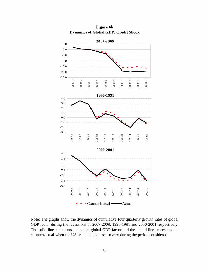
Figure 6b Dynamics of Global GDP: Credit Shock

Note: The graphs show the dynamics of cumulative four quarterly growth rates of global GDP factor during the recessions of 2007-2009, 1990-1991 and 2000-2001 respectively. The solid line represents the actual global GDP factor and the dotted line represents the counterfactual when the US credit shock is set to zero during the period considered.

2007-2009

-25.0

-20.0

-15.0

-10.0

-5.0

0.0

5.0

2007

:3

2007

:4

2008

:1

2008

:2

2008

:3

2008

:4

2009

:1

2009

:2

2009

:3

2009

:4

1990-1991

-3.0

-2.0

-1.0

0.01.0

2.0

3.0

4.0

1990

:1

1990

:2

1990

:3

1990

:4

1991

:1

1991

:2

1991

:3

1991

:4

1992

:1

1992

:22000-2001

-5.0

-3.5

-2.0

-0.5

1.0

2.5

4.0

2000

:4

2001

:1

2001

:2

2001

:3

2001

:4

2002

:1

2002

:2

2002

:3

2002

:4

2003

:1

Counterfactual Actual

- 35 -

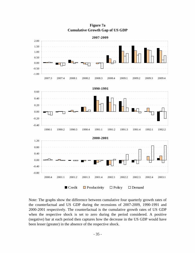
Figure 7a Cumulative Growth Gap of US GDP

Note: The graphs show the difference between cumulative four quarterly growth rates of the counterfactual and US GDP during the recessions of 2007-2009, 1990-1991 and 2000-2001 respectively. The counterfactual is the cumulative growth rates of US GDP when the respective shock is set to zero during the period considered. A positive (negative) bar at each period then captures how the decrease in the US GDP would have been lesser (greater) in the absence of the respective shock.

2007-2009

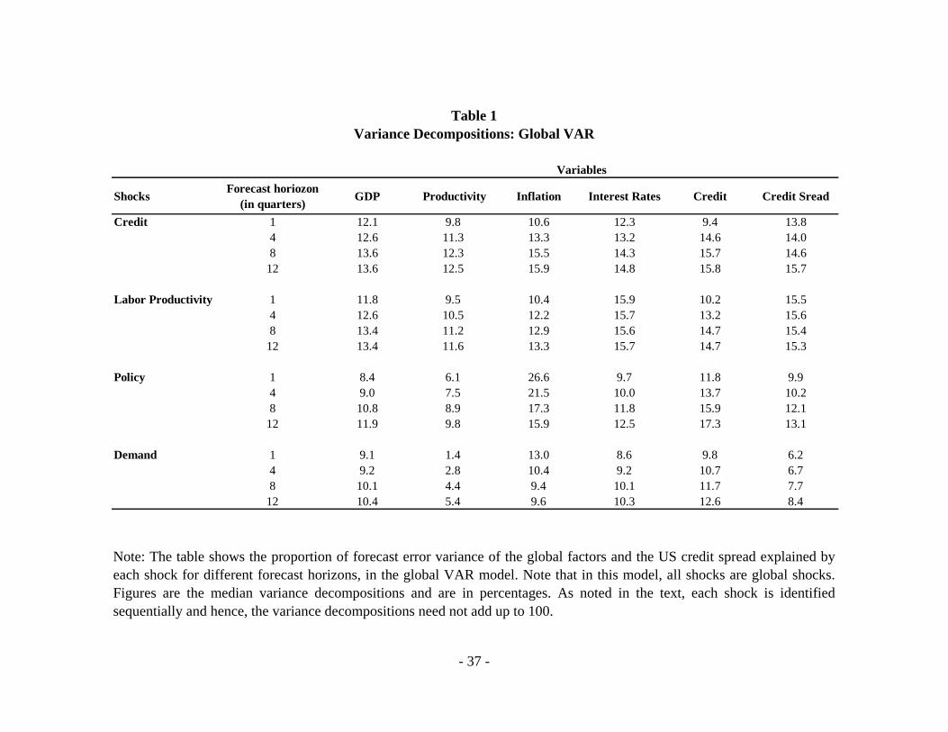
-1.00

-0.50

0.00

0.50

1.00

1.50

2.00

2007:3 2007:4 2008:1 2008:2 2008:3 2008:4 2009:1 2009:2 2009:3 2009:4

1990-1991

-0.40

-0.20

0.00

0.20

0.40

0.60

1990:1 1990:2 1990:3 1990:4 1991:1 1991:2 1991:3 1991:4 1992:1 1992:2

2000-2001

-0.80

-0.40

0.00

0.40

0.80

1.20

2000:4 2001:1 2001:2 2001:3 2001:4 2002:1 2002:2 2002:3 2002:4 2003:1

Credit Productivity Policy Demand

- 36 -

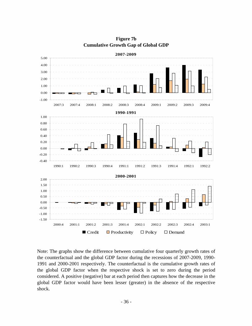
Figure 7b

Cumulative Growth Gap of Global GDP Note: The graphs show the difference between cumulative four quarterly growth rates of the counterfactual and the global GDP factor during the recessions of 2007-2009, 1990-1991 and 2000-2001 respectively. The counterfactual is the cumulative growth rates of the global GDP factor when the respective shock is set to zero during the period considered. A positive (negative) bar at each period then captures how the decrease in the global GDP factor would have been lesser (greater) in the absence of the respective shock.

2007-2009

-1.00

0.00

1.00

2.00

3.00

4.00

5.00

2007:3 2007:4 2008:1 2008:2 2008:3 2008:4 2009:1 2009:2 2009:3 2009:4

1990-1991

-0.40

-0.20

0.00

0.20

0.40

0.60

0.80

1.00

1990:1 1990:2 1990:3 1990:4 1991:1 1991:2 1991:3 1991:4 1992:1 1992:2

2000-2001

-1.50

-1.00

-0.50

0.00

0.50

1.00

1.50

2.00

2000:4 2001:1 2001:2 2001:3 2001:4 2002:1 2002:2 2002:3 2002:4 2003:1

Credit Productivity Policy Demand

- 37 -

Table 1 Variance Decompositions: Global VAR

Note: The table shows the proportion of forecast error variance of the global factors and the US credit spread explained by each shock for different forecast horizons, in the global VAR model. Note that in this model, all shocks are global shocks. Figures are the median variance decompositions and are in percentages. As noted in the text, each shock is identified sequentially and hence, the variance decompositions need not add up to 100.

Shocks Forecast horiozon (in quarters) GDP Productivity Inflation Interest Rates Credit Credit Sread

Credit 1 12.1 9.8 10.6 12.3 9.4 13.84 12.6 11.3 13.3 13.2 14.6 14.08 13.6 12.3 15.5 14.3 15.7 14.6

12 13.6 12.5 15.9 14.8 15.8 15.7

Labor Productivity 1 11.8 9.5 10.4 15.9 10.2 15.54 12.6 10.5 12.2 15.7 13.2 15.68 13.4 11.2 12.9 15.6 14.7 15.4

12 13.4 11.6 13.3 15.7 14.7 15.3

Policy 1 8.4 6.1 26.6 9.7 11.8 9.94 9.0 7.5 21.5 10.0 13.7 10.28 10.8 8.9 17.3 11.8 15.9 12.1

12 11.9 9.8 15.9 12.5 17.3 13.1

Demand 1 9.1 1.4 13.0 8.6 9.8 6.24 9.2 2.8 10.4 9.2 10.7 6.78 10.1 4.4 9.4 10.1 11.7 7.7

12 10.4 5.4 9.6 10.3 12.6 8.4

Variables

- 38 -

Table 2

Variance Decompositions: US FAVAR

Note: The table shows the proportion of forecast error variance of the US variables and the global GDP factor explained by each shock for different forecast horizons, in the US FAVAR model. Note that in this model, all shocks are US shocks. Figures are the median variance decompositions and are in percentages. As noted in the text, each shock is identified sequentially and hence, the variance decompositions need not add up to 100.

Shocks Forecast horiozon (in quarters) Global GDP GDP Productivity Inflation Interest Rates Credit Credit Spread

Credit 1 10.3 8.1 8.4 8.5 10.1 9.8 10.64 12.4 10.5 9.8 9.9 10.4 11.9 10.78 13.3 12.4 11.5 11.9 11.4 13.7 11.912 13.3 12.9 12.3 12.5 12.1 14.1 12.3

Labor Productivity 1 11.5 16.6 6.6 7.2 11.1 8.9 12.84 12.8 15.9 8.7 8.9 11.4 10.2 12.78 12.9 14.5 11.1 10.2 12.0 11.8 13.412 13.0 14.2 11.9 10.8 12.2 12.1 13.6

Policy 1 10.0 5.9 8.2 16.8 9.2 9.8 10.24 11.0 9.3 11.2 16.3 10.2 11.1 10.28 13.3 11.8 12.8 15.4 12.1 13.2 11.812 13.9 12.7 12.8 15.1 12.5 13.9 12.6

Demand 1 12.7 18.4 5.2 12.0 9.4 8.4 9.84 13.2 16.6 7.8 12.5 9.8 9.6 10.38 13.8 15.5 10.3 13.0 10.9 11.9 11.112 13.7 15.4 11.2 13.6 11.4 13.0 11.2

Variables

39

Appendix A

Country Source Source Base Database Code Description

Canada IFS EDSS IFTSTSUB 15664...ZF... CPI:ALL CITIES POP OVR.30,000France IFS EDSS IFTSTSUB 13264...ZF... CPI: 108 CITIESGermany IFS EDSS IFTSTSUB 13464...ZF... CPI Unified GermanyItaly IFS EDSS IFTSTSUB 13664...ZF... CPI:ALL ITALYJapan IFS EDSS IFTSTSUB 15864...ZF... CPI:ALL JAPAN-485 ITEMSUnited Kingdom IFS EDSS IFTSTSUB 11264...ZF... CPI: ALL ITEMSUnited States IFS EDSS IFTSTSUB 11164...ZF... CPI All ITEMS CITY AVERAGE

*Inflation was calculated as the year over year change in CPI

Country Source Source Base Database Code Description

Canada IFS EDSS IFTSTSUB 15660C..ZF... TREASURY BILL RATEFrance IFS EDSS IFTSTSUB 13260C..ZF... TREASURY BILLS:3 MONTHSGermany IFS EDSS IFTSTSUB 13460C..ZF... TREASURY BILL RATEItaly IFS EDSS IFTSTSUB 13660C..ZF... TREASURY BILL RATEJapan IFS EDSS IFTSTSUB 15860C..ZF... FINANCING BILL RATEUnited Kingdom IFS EDSS IFTSTSUB 11260C..ZF... TREASURY BILL RATEUnited States IFS EDSS IFTSTSUB 11160C..ZF... TREASURY BILL RATE

Inflation*

Nominal Short Term Interest Rate

40

Country Source Source Base Database Code Description

Canada OECD EDSS OETSADB 156.PDTY Labour productivity of the total economyFrance OECD EDSS OETSADB 132.PDTY Labour productivity of the total economyGermany OECD EDSS OETSADB 134.PDTY Labour productivity of the total economy

West Germany OECD EDSS OETSADB WGR.PDTY Labour productivity of the total economyItaly OECD EDSS OETSADB 136.PDTY Labour productivity of the total economyJapan OECD EDSS OETSADB 158.PDTY Labour productivity of the total economyUnited Kingdom OECD EDSS OETSADB 112.PDTY Labour productivity of the total economyUnited States OECD EDSS OETSADB 111.PDTY Labour productivity of the total economy

Country Source Source Base Database Code Description

Canada Statistics Canada Haver G10+ S156NGPC@G10 Gross Domestic Product (SAAR, Mil.Chn.2002.C$) France Institut National de la Statistique et

des Etudes EconomiquesHaver G10+ S132NGPC@G10 Gross Domestic Product (SA/WDA, Mil.Chn.2000.Euros)

Germany Deutsche Bundesbank Haver G10+ S134NGPC@G10 Gross Domestic Product (SA/WDA, Bil.Chn.2000.Euros) Italy Istituto Nazionale di Statistica Haver G10+ S136NGPC@G10 Gross Domestic Product (SA/WDA, Mil.Chn.2000.Euros) Japan Cabinet Office Haver G10+ S158NGPC@G10 Gross Domestic Product (SAAR, Bil.Chn.2000.Yen) United Kingdom Office for National Statistics Haver G10+ S112NGPC@G10 Gross Domestic Product (SA, Mil.Chained.2005.Pounds) United States Bureau of Economic Analysis Haver G10+ S111NGPC@G10 Gross Domestic Product (SAAR, Bil.Chn.2005$)

Labour Productivity

Gross Domestic Product

41

Country Source Source Base Database Code Description

Canada IFS EDSS IFTSTSUB 15622D..ZF... CLAIMS ON PRIVATE SECTORFrance IFS EDSS IFTSTSUB 13222D..ZF... CREDIT TO PRIVATE SECTORGermany IFS EDSS IFTSTSUB 13422D..ZF... CLAIMS ON OTH RESSID SECTORItaly IFS EDSS IFTSTSUB 13622D..ZF... CLAIMS ON OTHER RESIDENT SECTORSJapan IFS EDSS IFTSTSUB 15822D..ZF... CLAIMS ON PRIVATE SECTORUnited Kingdom IFS EDSS IFTSTSUB 11222D..ZF... CLAIMS ON PRIVATE SECTORUnited States IFS EDSS IFTSTSUB 11122D..ZF... CLAIMS ON PRIVATE SECTOR

Country Source Code Description

Spread Calculated (Baa Interest Rate- Aaa Interest Rate)

Baa Moody's Investor Services. BAA Moody's Seasoned Baa Corporate Bond YieldAaa Moody's Investor Services. AAA Moody's Seasoned Aaa Corporate Bond Yield

Note: To complete the data for some series we also use other databases. Details of this are available form the authors on request.

SpreadSource Base

Board of Governors of the Board of Governors of the

Credit

- 42 -

Appendix B

Figure B1 Impulse Responses due to a Productivity Shock: Global VAR

Note: The graphs show the impulse responses of the global factors and the US credit spread due to a 1 standard deviation productivity shock in the global VAR model. The solid line represents the median and the dotted lines represent the 16th and the 84th percentiles based on 5000 draws.

Productivity

-0.8

-0.4

0.0

0.4

0.8

0 1 2 3 4 5 6 7 8 9 10 11

Inflation

-0.9

-0.6

-0.3

0.0

0.3

0 1 2 3 4 5 6 7 8 9 10 11

Credit

-1.2

-0.6

0.0

0.6

1.2

1.8

2.4

0 1 2 3 4 5 6 7 8 9 10 11

Credit Spread

-0.2

-0.1

-0.1

0.0

0.1

0.1

0 1 2 3 4 5 6 7 8 9 10 11

GDP

-0.8

-0.4

0.0

0.4

0.8

1.2

0 1 2 3 4 5 6 7 8 9 10 11

Interest Rates

-0.5

-0.3

0.0

0.3

0.5

0 1 2 3 4 5 6 7 8 9 10 11

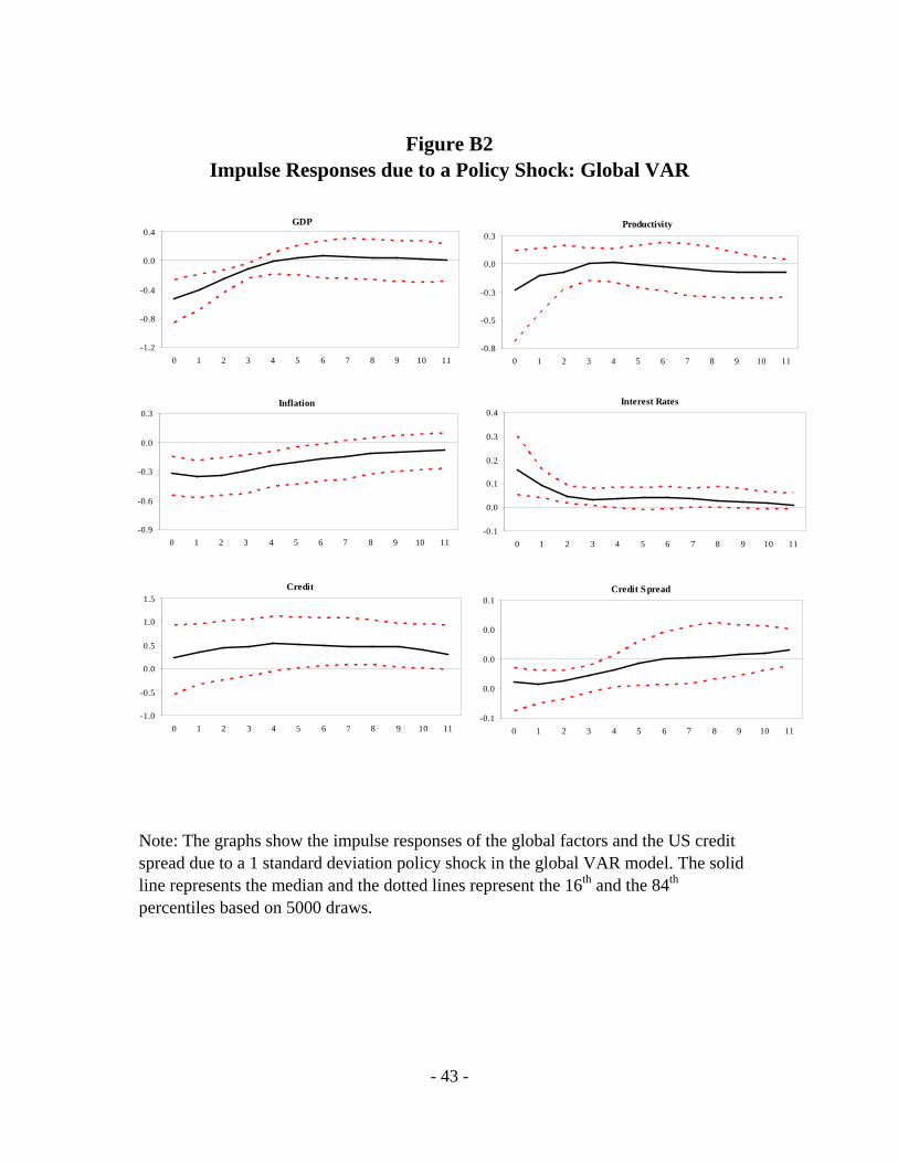
- 43 -

Figure B2

Impulse Responses due to a Policy Shock: Global VAR Note: The graphs show the impulse responses of the global factors and the US credit spread due to a 1 standard deviation policy shock in the global VAR model. The solid line represents the median and the dotted lines represent the 16th and the 84th percentiles based on 5000 draws.

Productivity

-0.8

-0.5

-0.3

0.0

0.3

0 1 2 3 4 5 6 7 8 9 10 11

GDP

-1.2

-0.8

-0.4

0.0

0.4

0 1 2 3 4 5 6 7 8 9 10 11

Inflation

-0.9

-0.6

-0.3

0.0

0.3

0 1 2 3 4 5 6 7 8 9 10 11

Credit

-1.0

-0.5

0.0

0.5

1.0

1.5

0 1 2 3 4 5 6 7 8 9 10 11

Credit Spread

-0.1

0.0

0.0

0.0

0.1

0 1 2 3 4 5 6 7 8 9 10 11

Interest Rates

-0.1

0.0

0.1

0.2

0.3

0.4

0 1 2 3 4 5 6 7 8 9 10 11

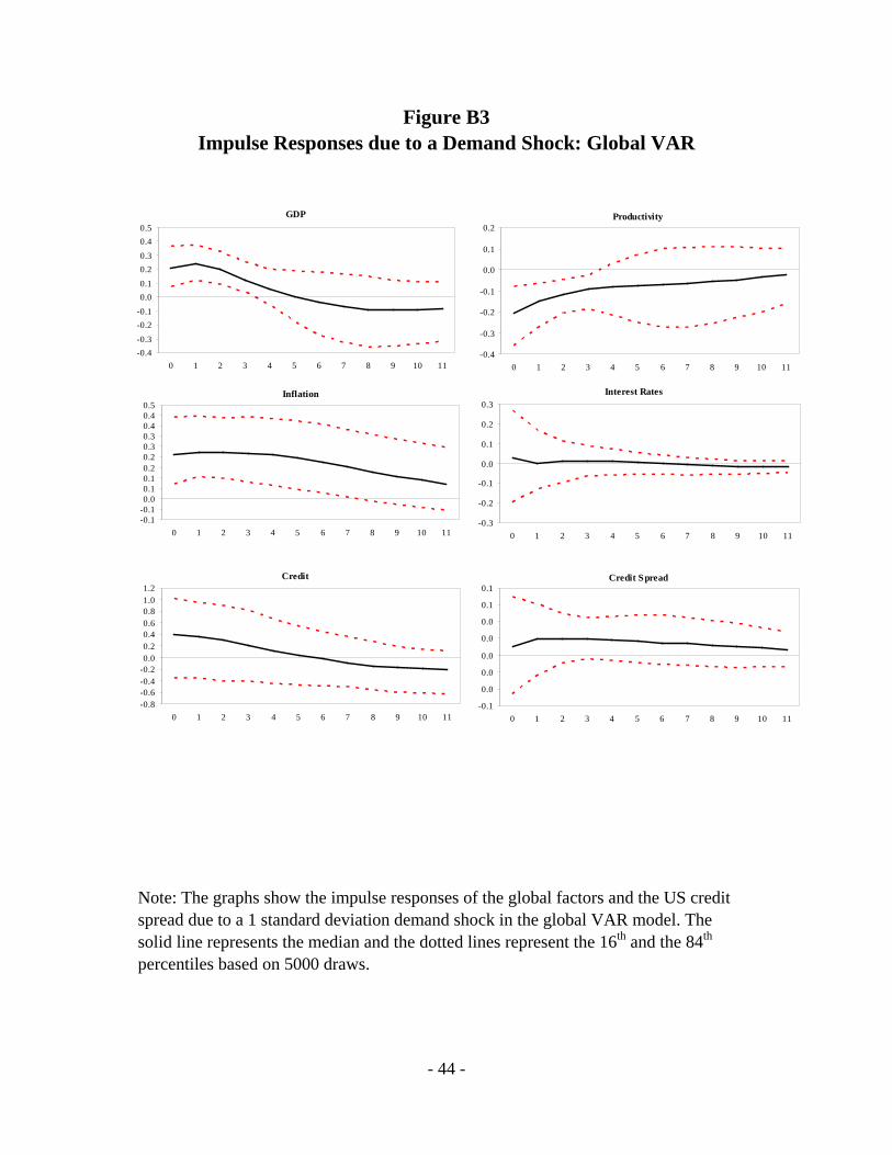
- 44 -

Figure B3 Impulse Responses due to a Demand Shock: Global VAR

Note: The graphs show the impulse responses of the global factors and the US credit spread due to a 1 standard deviation demand shock in the global VAR model. The solid line represents the median and the dotted lines represent the 16th and the 84th percentiles based on 5000 draws.

Productivity

-0.4

-0.3

-0.2

-0.1

0.0

0.1

0.2

0 1 2 3 4 5 6 7 8 9 10 11

GDP

-0.4-0.3-0.2-0.10.00.10.20.30.40.5

0 1 2 3 4 5 6 7 8 9 10 11

Inflation

-0.1-0.10.00.10.10.20.20.30.30.40.40.5

0 1 2 3 4 5 6 7 8 9 10 11

Credit

-0.8-0.6-0.4-0.20.00.20.40.60.81.01.2

0 1 2 3 4 5 6 7 8 9 10 11

Credit Spread

-0.1

0.0

0.0

0.0

0.0

0.0

0.1

0.1

0 1 2 3 4 5 6 7 8 9 10 11

Interest Rates

-0.3

-0.2

-0.1

0.0

0.1

0.2

0.3

0 1 2 3 4 5 6 7 8 9 10 11

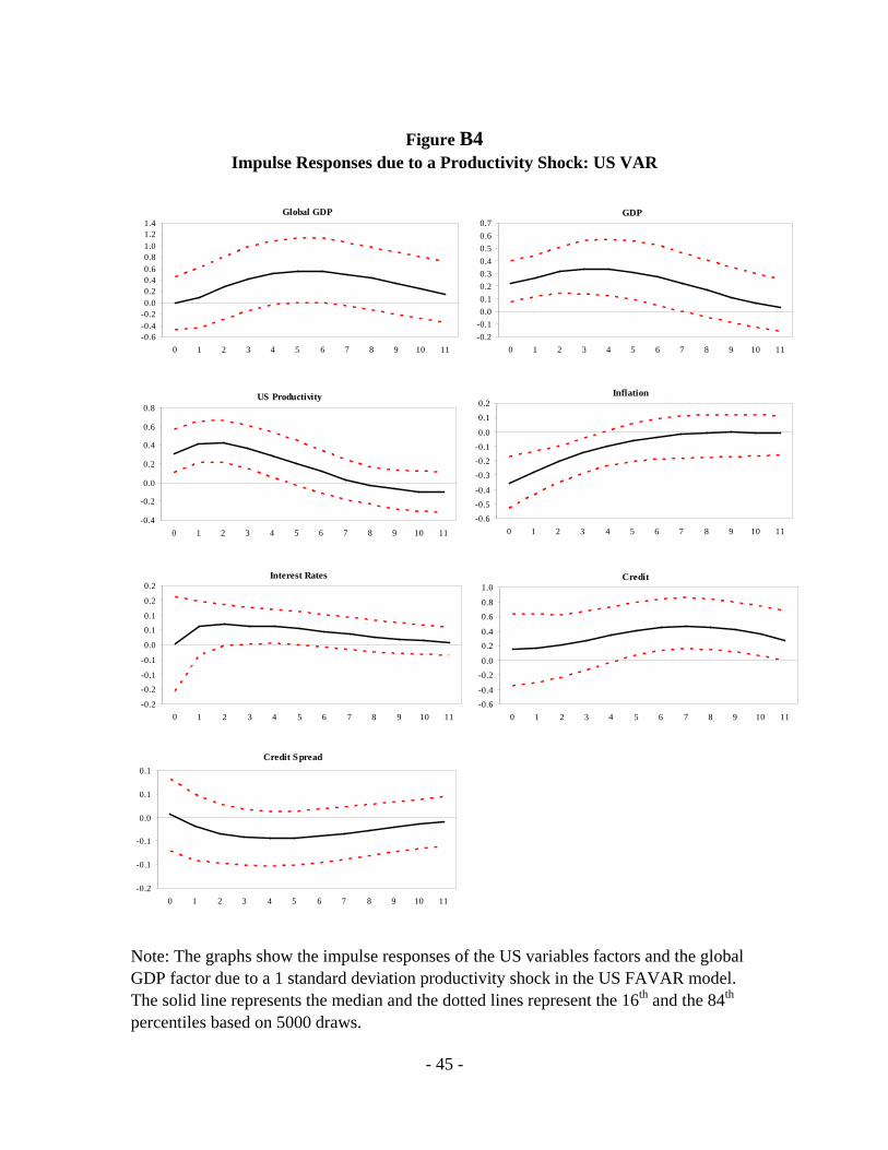
- 45 -

Figure B4

Impulse Responses due to a Productivity Shock: US VAR Note: The graphs show the impulse responses of the US variables factors and the global GDP factor due to a 1 standard deviation productivity shock in the US FAVAR model. The solid line represents the median and the dotted lines represent the 16th and the 84th percentiles based on 5000 draws.

US Productivity

-0.4

-0.2

0.0

0.2

0.4

0.6

0.8

0 1 2 3 4 5 6 7 8 9 10 11

GDP

-0.2-0.10.00.10.20.30.40.50.60.7

0 1 2 3 4 5 6 7 8 9 10 11

Inflation

-0.6-0.5-0.4

-0.3-0.2-0.10.0

0.10.2

0 1 2 3 4 5 6 7 8 9 10 11

Global GDP

-0.6-0.4-0.20.00.20.40.60.81.01.21.4

0 1 2 3 4 5 6 7 8 9 10 11

Credit

-0.6-0.4

-0.20.0

0.20.4

0.60.8

1.0

0 1 2 3 4 5 6 7 8 9 10 11

Credit Spread

-0.2

-0.1

-0.1

0.0

0.1

0.1

0 1 2 3 4 5 6 7 8 9 10 11

Interest Rates

-0.2

-0.2-0.1

-0.1

0.0

0.10.1

0.2

0.2

0 1 2 3 4 5 6 7 8 9 10 11

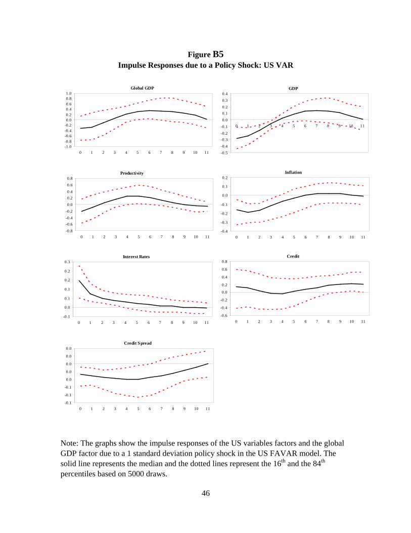
46

Figure B5 Impulse Responses due to a Policy Shock: US VAR

Note: The graphs show the impulse responses of the US variables factors and the global GDP factor due to a 1 standard deviation policy shock in the US FAVAR model. The solid line represents the median and the dotted lines represent the 16th and the 84th percentiles based on 5000 draws.

Productivity

-0.8-0.6-0.4-0.20.00.20.40.60.8

0 1 2 3 4 5 6 7 8 9 10 11

GDP

-0.5-0.4-0.3-0.2-0.10.00.10.20.30.4

0 1 2 3 4 5 6 7 8 9 10 11

Global GDP

-1.0-0.8-0.6-0.4-0.20.00.20.40.60.81.0

0 1 2 3 4 5 6 7 8 9 10 11

Inflation

-0.4

-0.3

-0.2

-0.1

0.0

0.1

0.2

0 1 2 3 4 5 6 7 8 9 10 11

Credit

-0.6

-0.4

-0.2

0.0

0.2

0.4

0.6

0.8

0 1 2 3 4 5 6 7 8 9 10 11

Credit Spread

-0.1

-0.1

-0.1

0.0

0.0

0.0

0.0

0.0

0 1 2 3 4 5 6 7 8 9 10 11

Interest Rates

-0.1

0.0

0.1

0.1

0.2

0.2

0.3

0 1 2 3 4 5 6 7 8 9 10 11

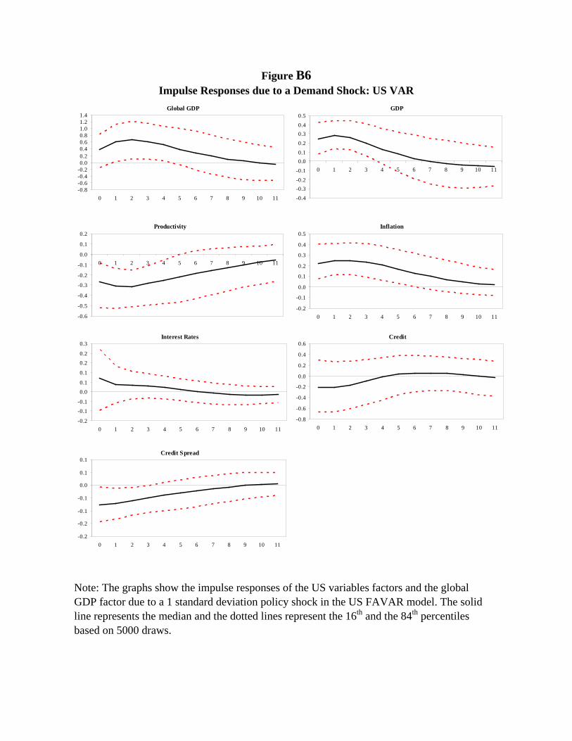
Figure B6 Impulse Responses due to a Demand Shock: US VAR

Note: The graphs show the impulse responses of the US variables factors and the global GDP factor due to a 1 standard deviation policy shock in the US FAVAR model. The solid line represents the median and the dotted lines represent the 16th and the 84th percentiles based on 5000 draws.

Productivity

-0.6

-0.5

-0.4

-0.3

-0.2

-0.1

0.0

0.1

0.2

0 1 2 3 4 5 6 7 8 9 10 11

GDP

-0.4-0.3-0.2-0.10.00.10.20.30.40.5

0 1 2 3 4 5 6 7 8 9 10 11

Global GDP

-0.8-0.6-0.4-0.20.00.20.40.60.81.01.21.4

0 1 2 3 4 5 6 7 8 9 10 11

Inflation

-0.2

-0.1

0.0

0.1

0.2

0.3

0.4

0.5

0 1 2 3 4 5 6 7 8 9 10 11

Credit

-0.8

-0.6

-0.4

-0.2

0.0

0.2

0.4

0.6

0 1 2 3 4 5 6 7 8 9 10 11

Credit Spread

-0.2

-0.2

-0.1

-0.1

0.0

0.1

0.1

0 1 2 3 4 5 6 7 8 9 10 11

Interest Rates

-0.2

-0.1-0.1

0.00.1

0.1

0.20.2

0.3

0 1 2 3 4 5 6 7 8 9 10 11