Dissolutive Wetting: What Controls Spreading?
52
Dissolutive Wetting: What Controls Spreading? James A. Warren, NIST Daniel Wheeler, NIST William Boettinger, NIST Modeling the early stages of reactive wetting, Daniel Wheeler, James A. Warren and William J. Boettinger, PRE (accepted, finally!) 2010 Thursday, October 28, 2010
Transcript of Dissolutive Wetting: What Controls Spreading?
Dissolutive Wetting:What Controls Spreading?James A. Warren, NIST
Daniel Wheeler, NIST
William Boettinger, NIST
Modeling the early stages of reactive wetting,Daniel Wheeler, James A. Warren and William J.
Boettinger,PRE (accepted, finally!) 2010
Thursday, October 28, 2010
OutlineMotivation
Methods, Limitations of prior efforts
Hydrodynamics, Low Ohnesorge Number flow
Numerics
Thick interfaces and intitial conditions
New metrics of spreading
Thursday, October 28, 2010
Good old Wetting
γLS
γLI γSI γSIγLI
γLS
ψ
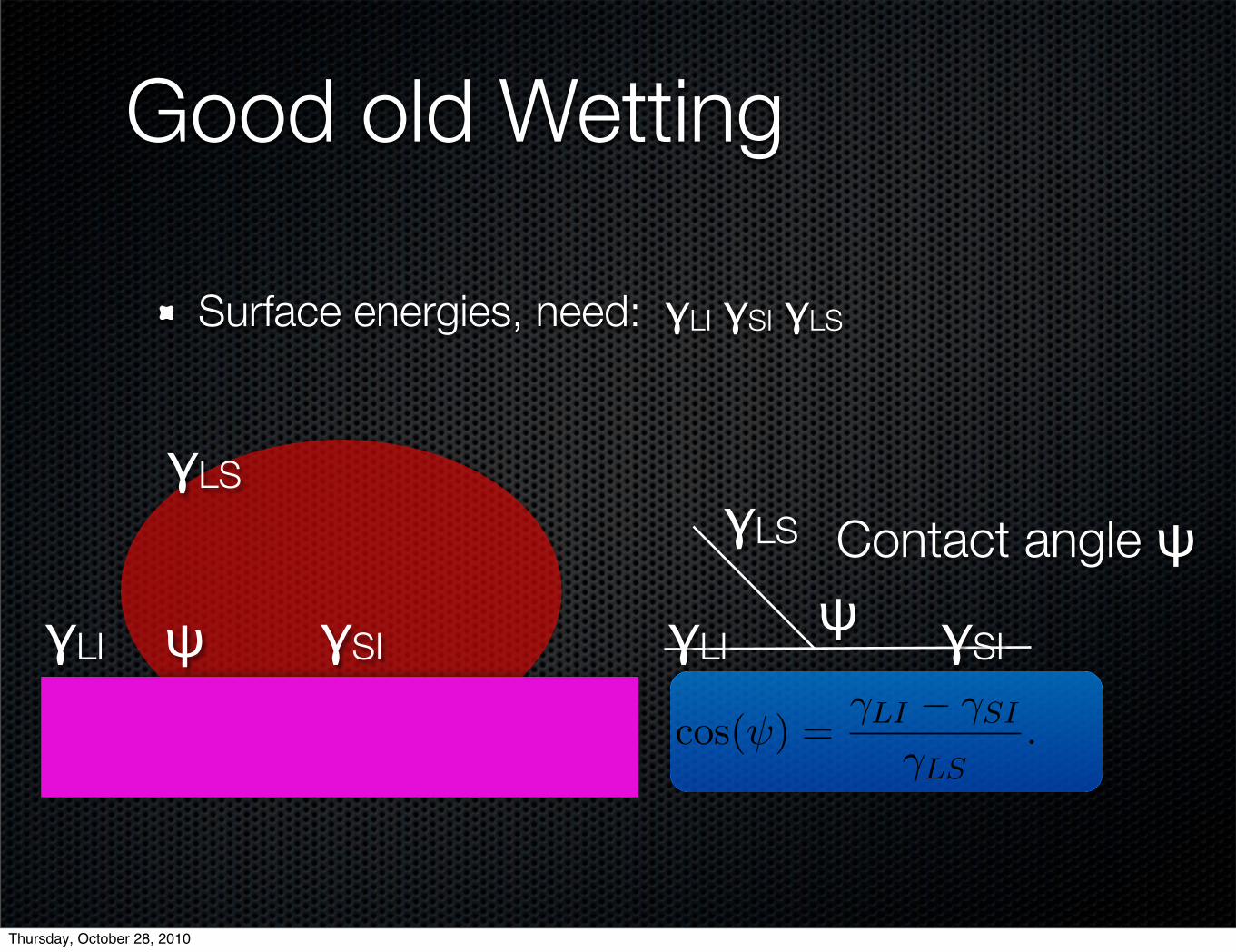
2.2 Surface Energies and Contact Angles
Finally, we may compute the surface energies for a liquid-solid (γLS), liquid-inert (γLI), and solid-inert (γSI) boundaries, and from this compute thecontact angle of a solid-liquid-intert triple junction. Using Fig. 2 as aschematic guide to determine the contact angle, ψ, between the solid-liquidsurface and the intert material (with the angle subtending the solid material)we find a version of the Young-Laplace Equation:
cos(ψ) =γLI − γSI
γLS. (20)
The surface energies can be computed using the first integral and argumentsfound in a number of sources **Wheeler Reference**, **Plapp Reference**and others. In general the surface energy between any two phases A and Bwill be
γAB = 2� ∞
−∞dx [f − f∞ − µc] (21)
Typically, we would now be forced to numerical methods to computethe surface energies, but we note that the work of Folch and Plapp picksa particular form for the free energy density that allows for further ana-lyitic progress for the case of an alloy. Specifically, we select a free energyf(φS ,φI , c) to be
f(φS , 0, c) = WG(φS) + X
�12
(c−AL(T )(1− p(φS)))2 + BL(T )(1− p(φS))�
,
f(φS , 1) = f∞, (22)
where G(φS) is a double-well with minima at φS = 0, 1, W is the scale ofthe height of the double well, X is an energy scale associated with chemicalchanges in the system, and p(φS) is an interpolating function between phaseswith p(0) = 0 and p(1) = 1. The parameters AL(T ) and BL(T ) are functionsof temperature, T , (which has been assumed isotropic), and can be used tofit to a variety of realistic phase diagrams. The above form as the advantagethat, when differentiated with respect to c gives
µ
X=
∂f
∂c= c−AL(1− p(φS)), (23)
which in equlibrium means we can trivially compute c, given φS . We defineequilibrium between solid and liquid by the requirement that µ is a constantin all the phases and the change in free energy between phases is µ(cL− cS),
5
Surface energies, need: γLI γSI γLS
ψ
Contact angle ψ
Thursday, October 28, 2010
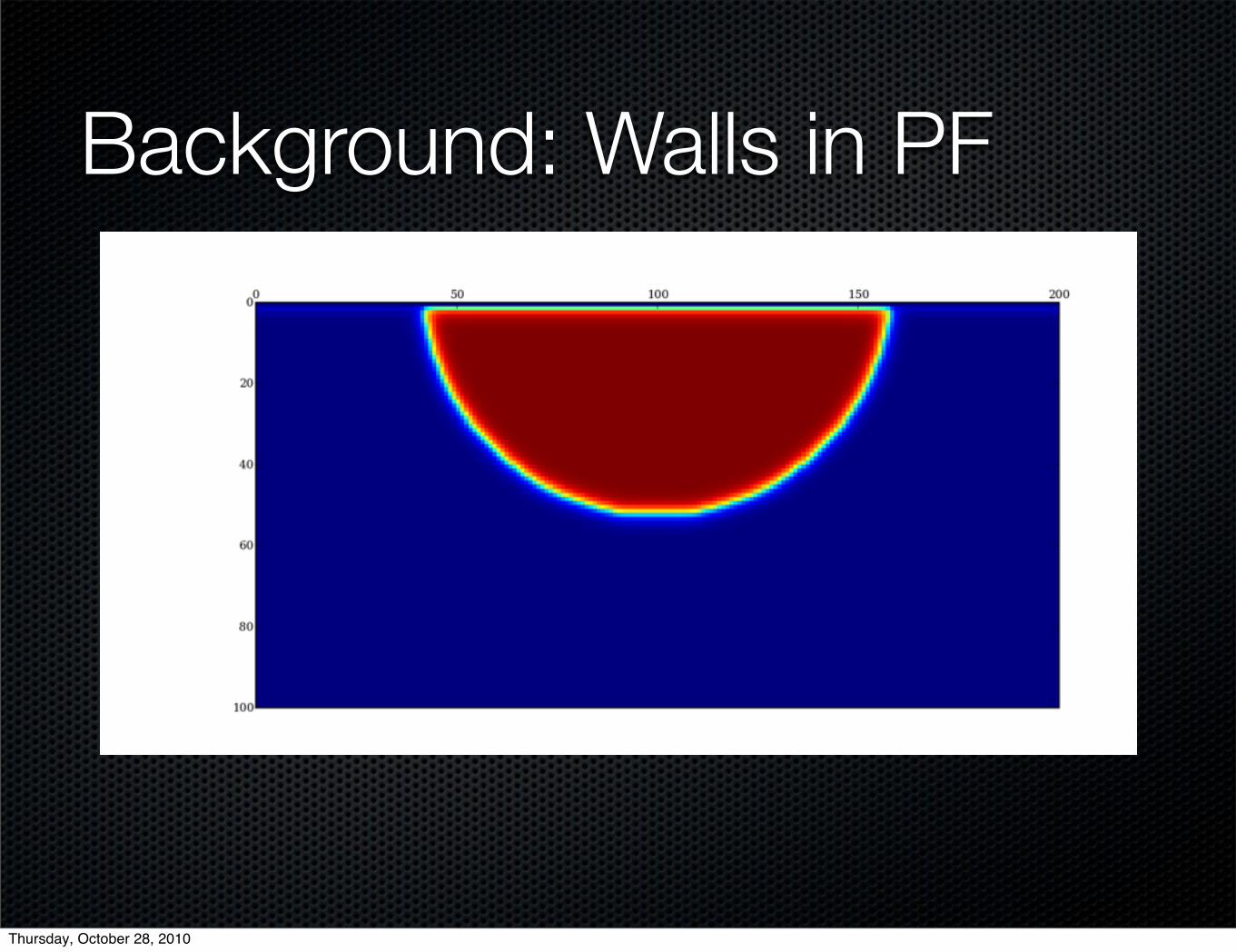
Background: Walls in PF
Thursday, October 28, 2010
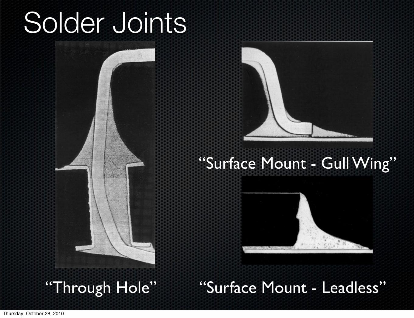
Solder Joints
“Through Hole”
“Surface Mount - Gull Wing”
“Surface Mount - Leadless”Thursday, October 28, 2010
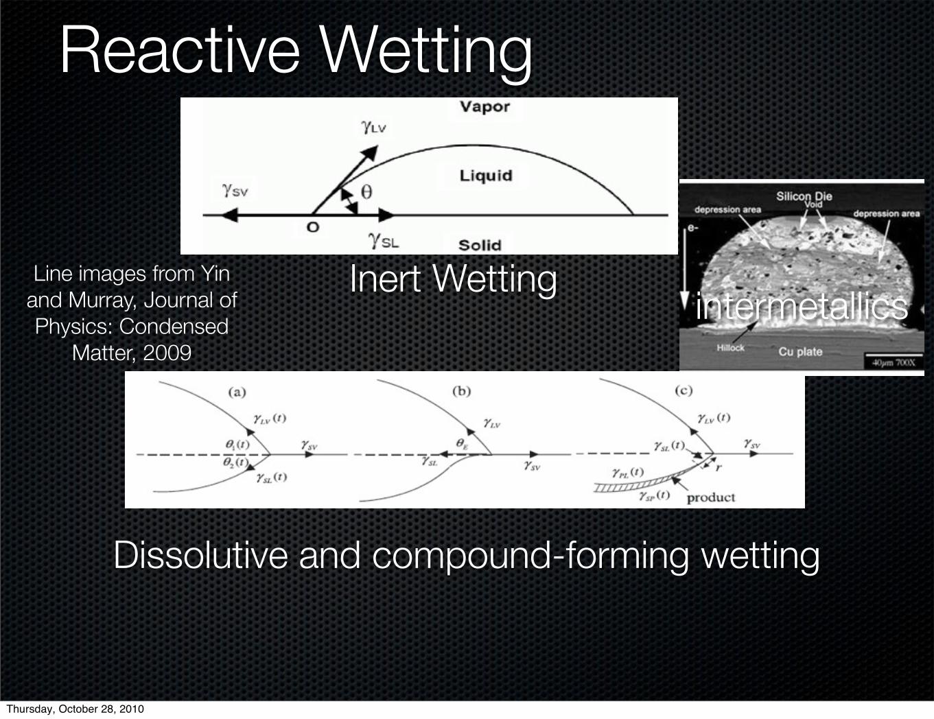
Reactive Wetting
Inert Wetting
Dissolutive and compound-forming wetting
Line images from Yin and Murray, Journal of Physics: Condensed
Matter, 2009
intermetallics
Thursday, October 28, 2010
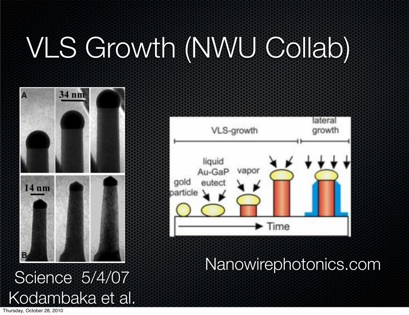
VLS Growth (NWU Collab)
Science 5/4/07 Kodambaka et al.
Nanowirephotonics.com
Thursday, October 28, 2010
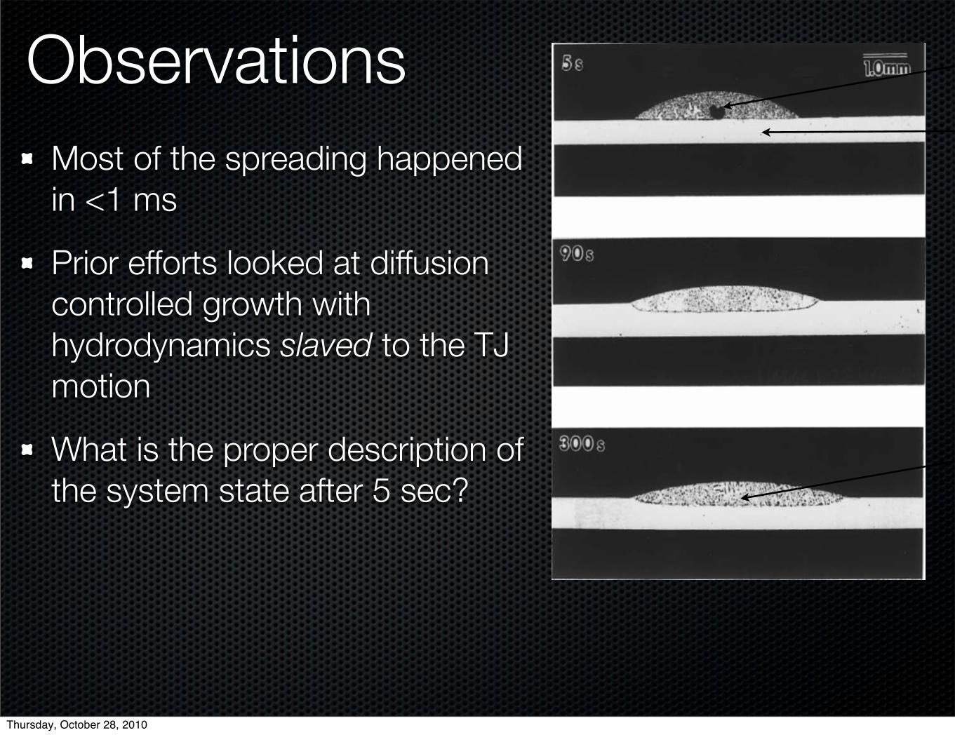
ObservationsMost of the spreading happened in <1 ms
Prior efforts looked at diffusion controlled growth with hydrodynamics slaved to the TJ motion
What is the proper description of the system state after 5 sec?
Thursday, October 28, 2010
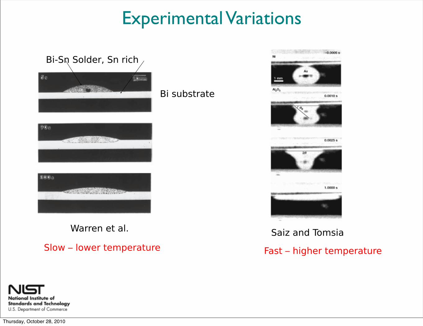
Experimental Variations
Saiz and TomsiaWarren et al.
Bi-Sn Solder, Sn rich
Bi substrate
Slow – lower temperature Fast – higher temperature
Thursday, October 28, 2010
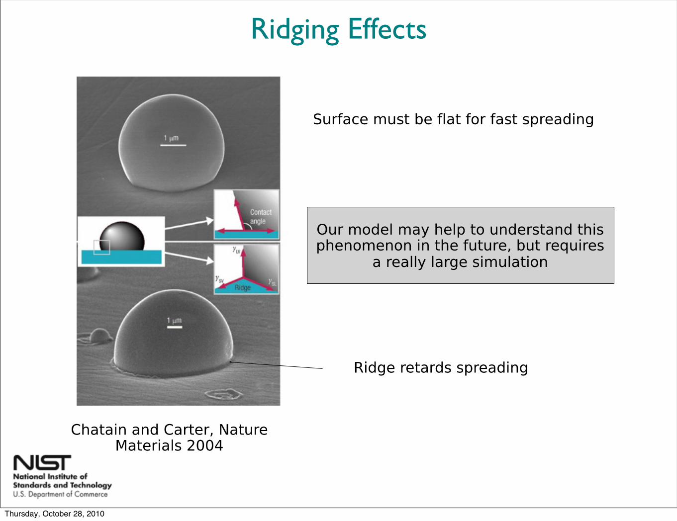
Ridging Effects
Ridge retards spreading
Surface must be flat for fast spreading
Chatain and Carter, Nature Materials 2004
Our model may help to understand this phenomenon in the future, but requires
a really large simulation
Thursday, October 28, 2010
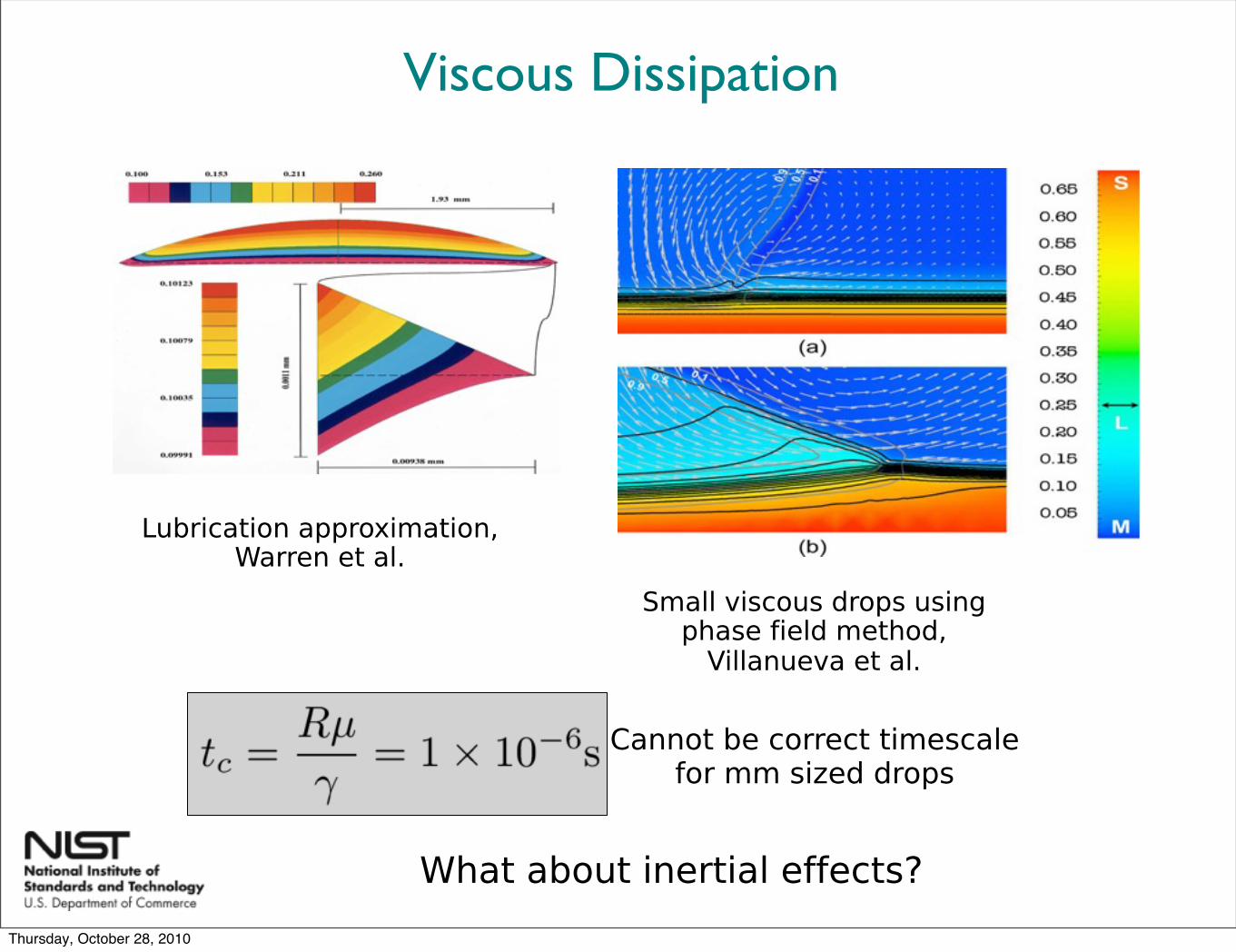
Viscous Dissipation
Lubrication approximation, Warren et al.
What about inertial effects?
Small viscous drops using phase field method,
Villanueva et al.
Cannot be correct timescale for mm sized drops
Thursday, October 28, 2010
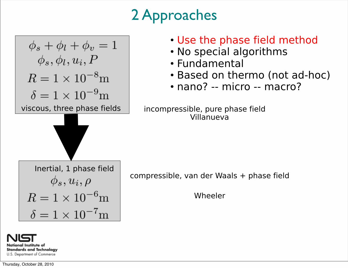
Use the phase field method No special algorithms Fundamental Based on thermo (not ad-hoc) nano? -- micro -- macro?
2 Approaches
viscous, three phase fields
Inertial, 1 phase field
Villanueva
Wheeler
incompressible, pure phase field
compressible, van der Waals + phase field
Thursday, October 28, 2010
Outline
Motivation and Introduction Phase Field Method intro/Fundamentals Thermodynamic derivation Numerical approach (FiPy digression) Results Conclusions
Thursday, October 28, 2010
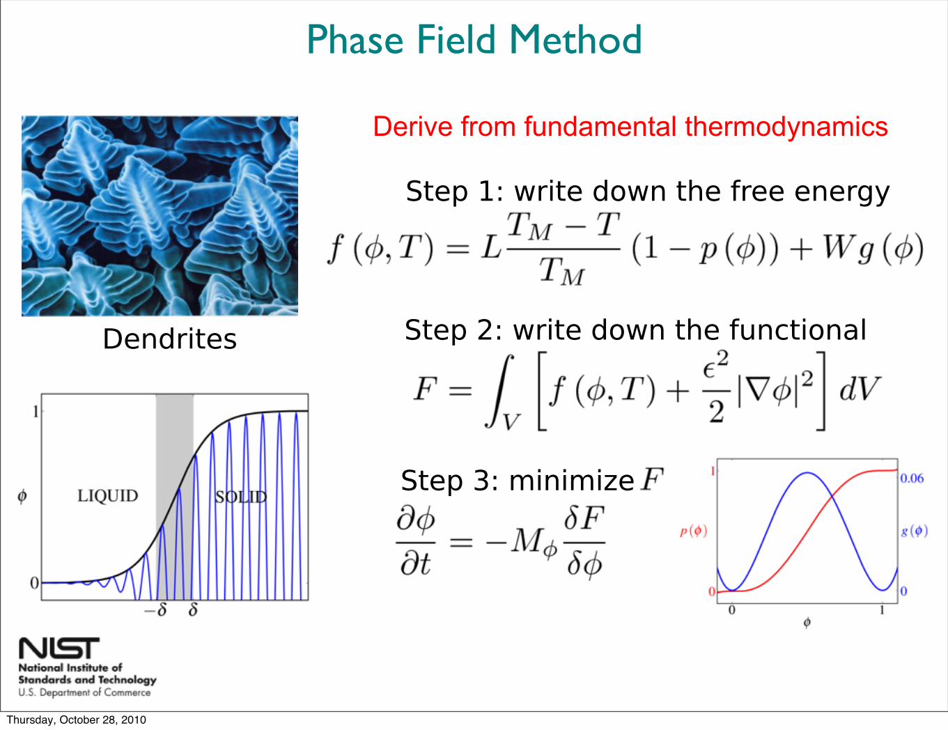
Phase Field Method
Dendrites
Derive from fundamental thermodynamics
Step 1: write down the free energy
Step 2: write down the functional
Step 3: minimize
Thursday, October 28, 2010
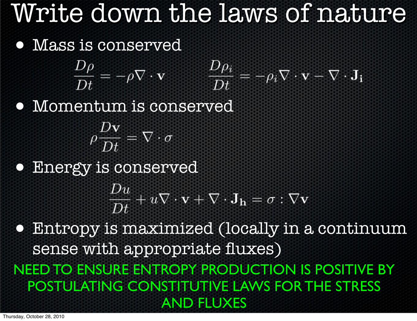
Write down the laws of nature• Mass is conserved
• Momentum is conserved
• Energy is conserved
• Entropy is maximized (locally in a continuum sense with appropriate fluxes)
NEED TO ENSURE ENTROPY PRODUCTION IS POSITIVE BYPOSTULATING CONSTITUTIVE LAWS FOR THE STRESS
AND FLUXESThursday, October 28, 2010
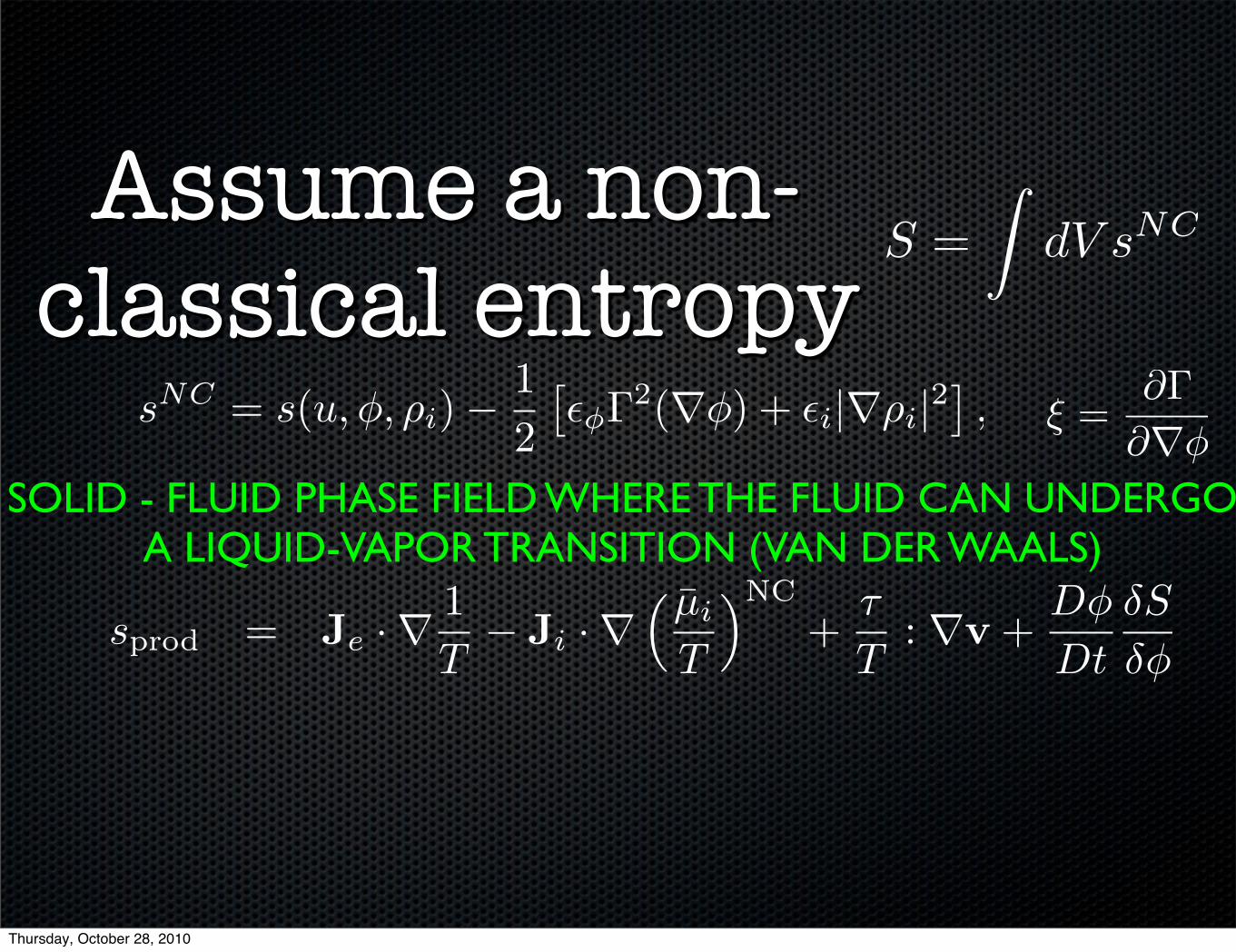
Assume a non-classical entropy
SOLID - FLUID PHASE FIELD WHERE THE FLUID CAN UNDERGO A LIQUID-VAPOR TRANSITION (VAN DER WAALS)
S =�
dV sNC
sNC = s(u, φ, ρi)−12
��φΓ2(∇φ) + �i|∇ρi|2
�, ξ =
∂Γ∂∇φ
sprod = Je ·∇ 1T− Ji ·∇
� µ̄i
T
�NC
+τ
T: ∇v +
Dφ
Dt
δS
δφ
Thursday, October 28, 2010
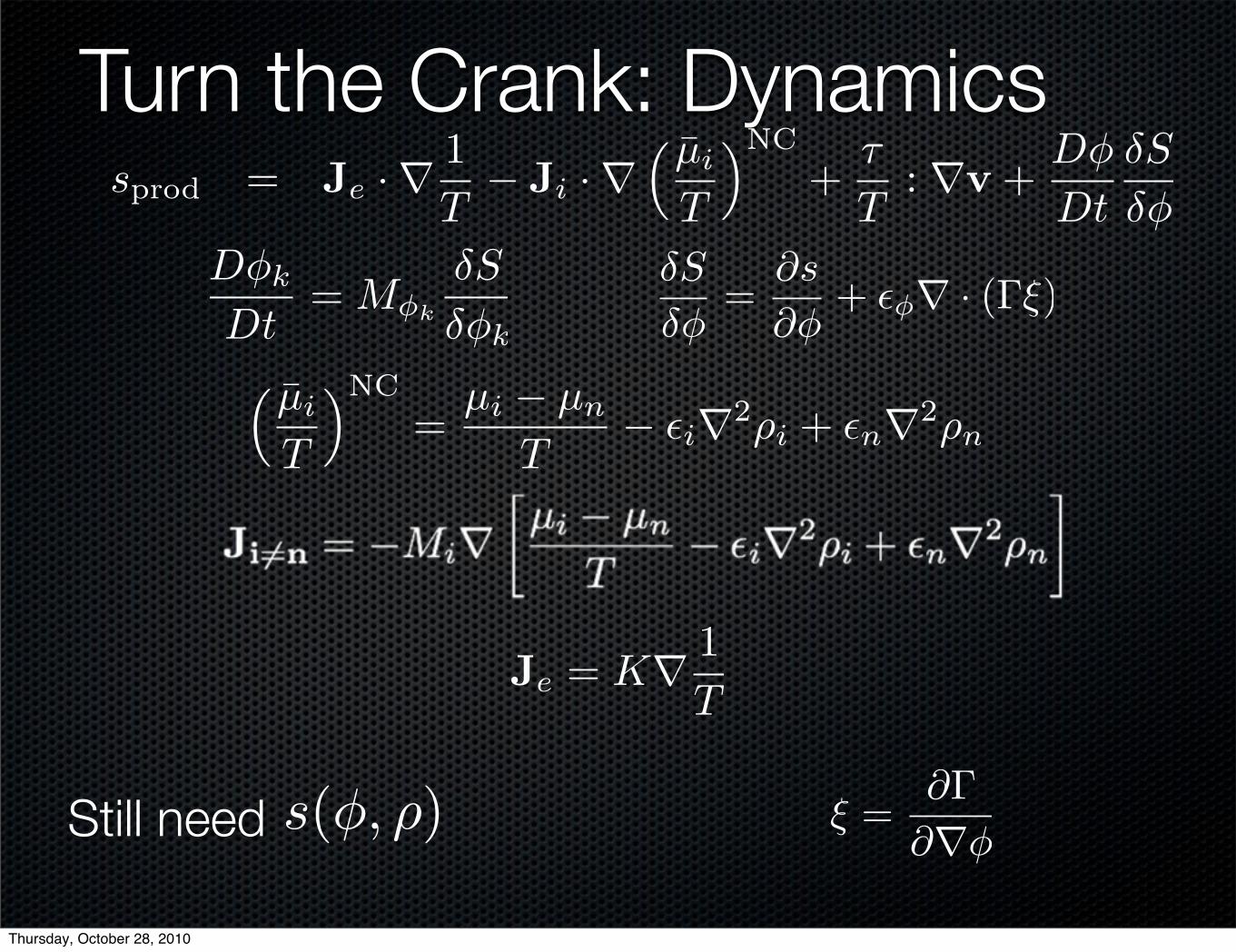
Turn the Crank: Dynamics
Dφk
Dt= Mφk
δS
δφk
sprod = Je ·∇ 1T− Ji ·∇
� µ̄i
T
�NC
+τ
T: ∇v +
Dφ
Dt
δS
δφ
Je = K∇ 1T
δS
δφ=
∂s
∂φ+ �φ∇ · (Γξ)
� µ̄i
T
�NC
=µi − µn
T− �i∇2ρi + �n∇2ρn
ξ =∂Γ
∂∇φStill need s(φ, ρ)
Thursday, October 28, 2010
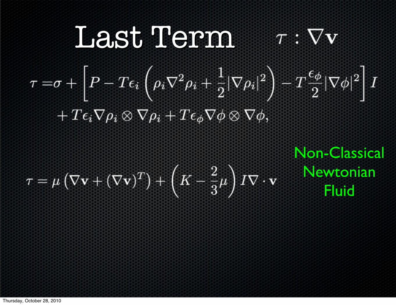
Last Term
Non-ClassicalNewtonian
Fluid
Thursday, October 28, 2010
Outline
Motivation and introduction Phase field method intro Thermodynamics (local) Numerical approach (FiPy digression) Results Conclusions
Thursday, October 28, 2010
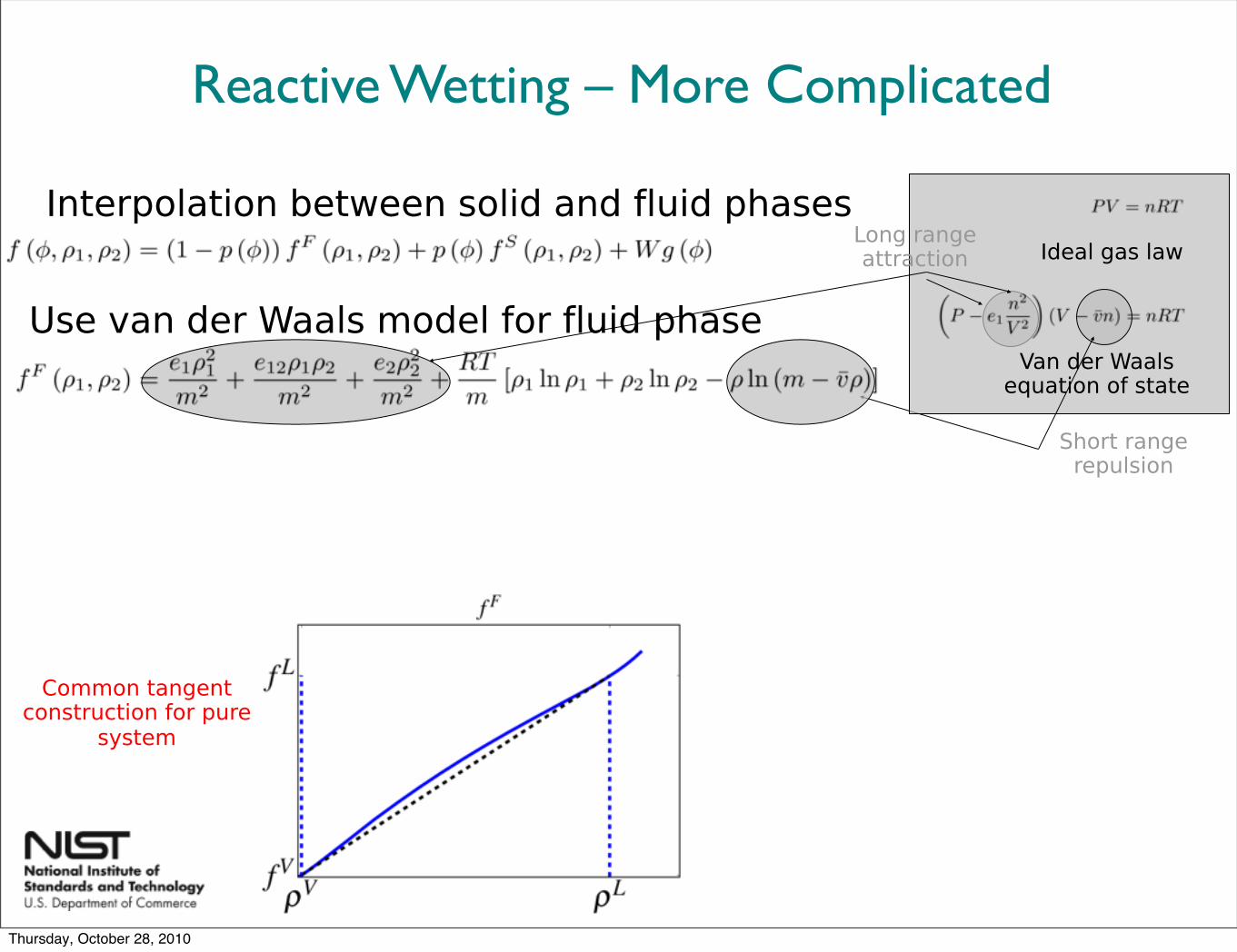
Short range repulsion
Reactive Wetting – More Complicated
Common tangent construction for pure
system
Interpolation between solid and fluid phases
Use van der Waals model for fluid phase
Ideal gas law
Van der Waals equation of state
Long range attraction
Thursday, October 28, 2010
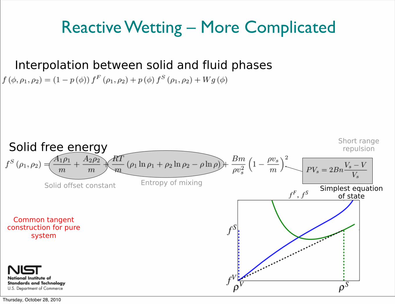
Short range repulsion
Reactive Wetting – More Complicated
Common tangent construction for pure
system
Interpolation between solid and fluid phases
Solid free energy
Entropy of mixingSolid offset constant Simplest equation of state
Thursday, October 28, 2010
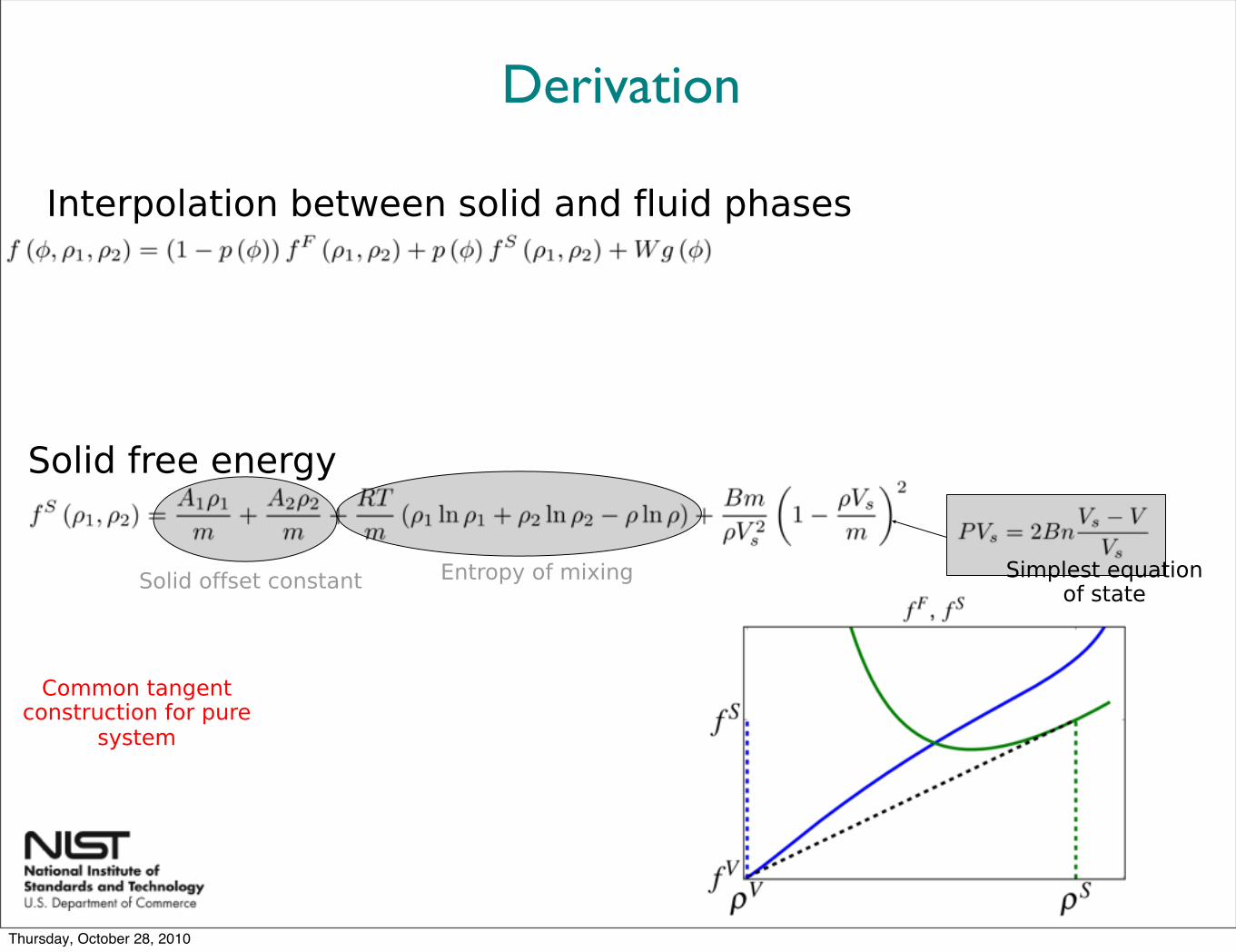
Derivation
Common tangent construction for pure
system
Interpolation between solid and fluid phases
Solid free energy
Entropy of mixingSolid offset constant Simplest equation of state
Thursday, October 28, 2010
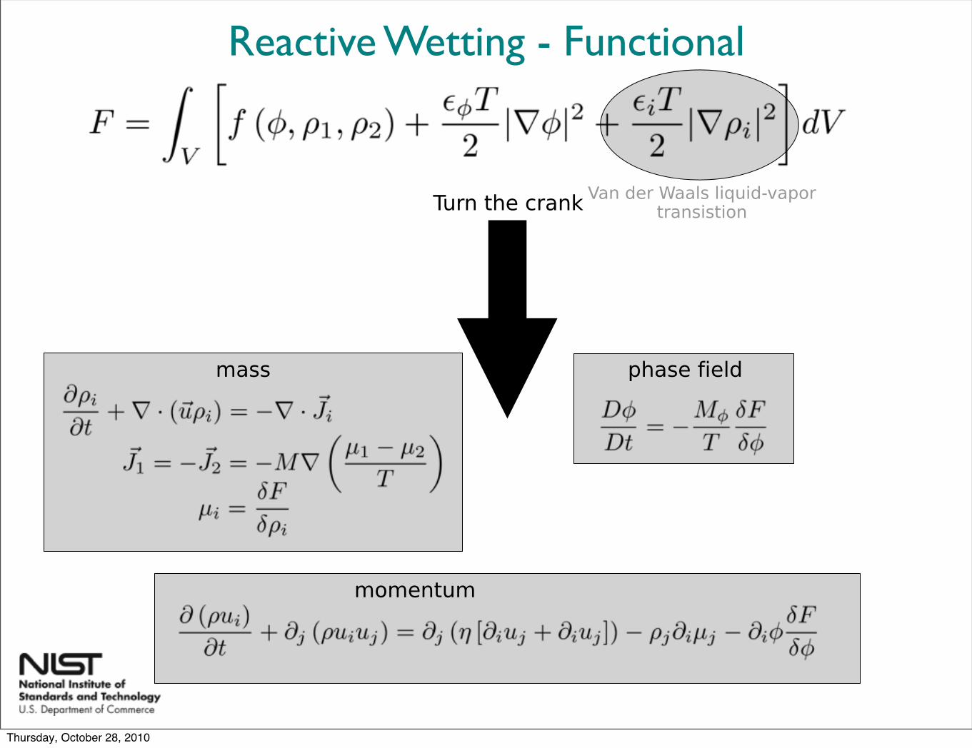
Reactive Wetting - Functional
Van der Waals liquid-vapor transistion
mass phase field
momentum
Turn the crank
Thursday, October 28, 2010
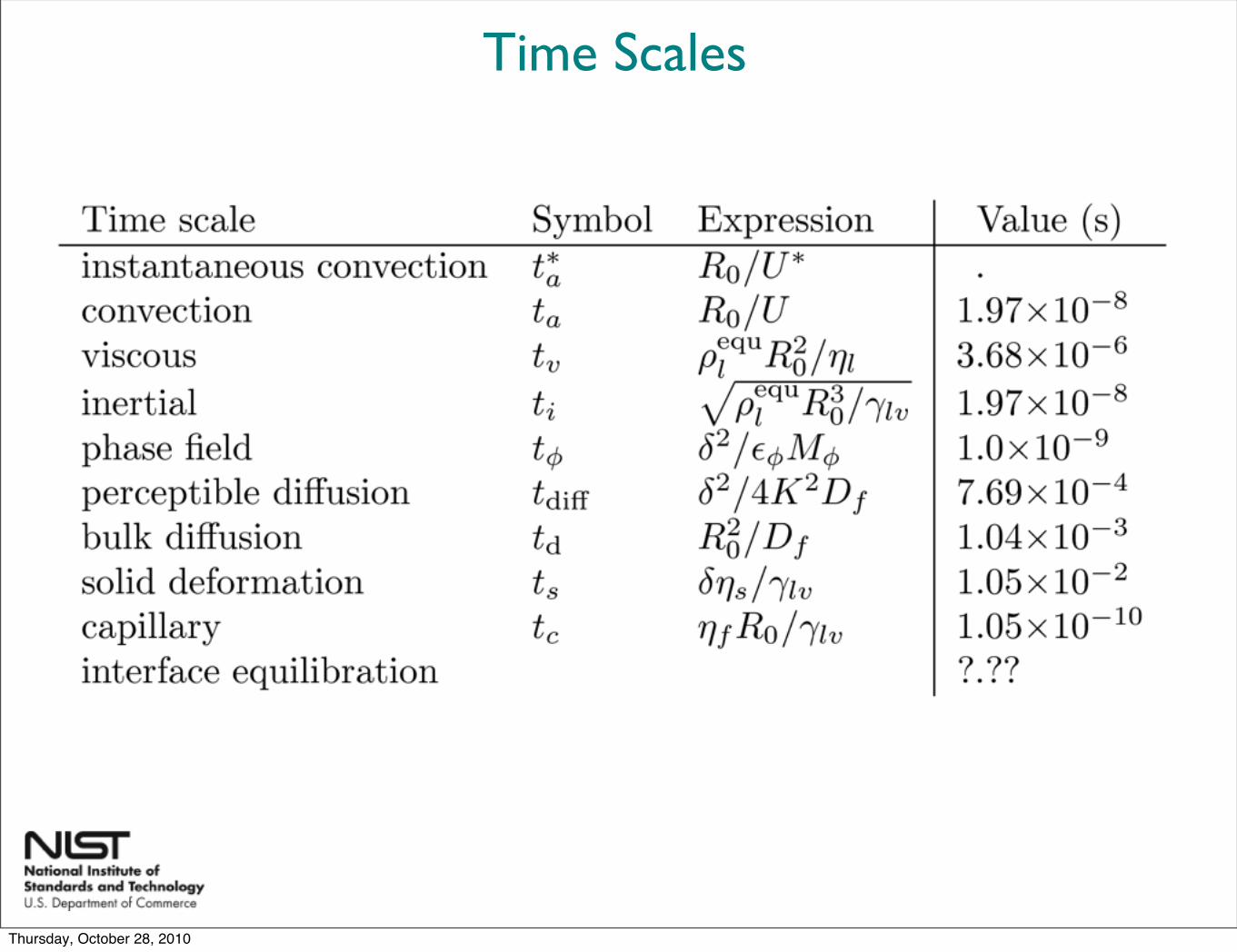
Time Scales
Thursday, October 28, 2010
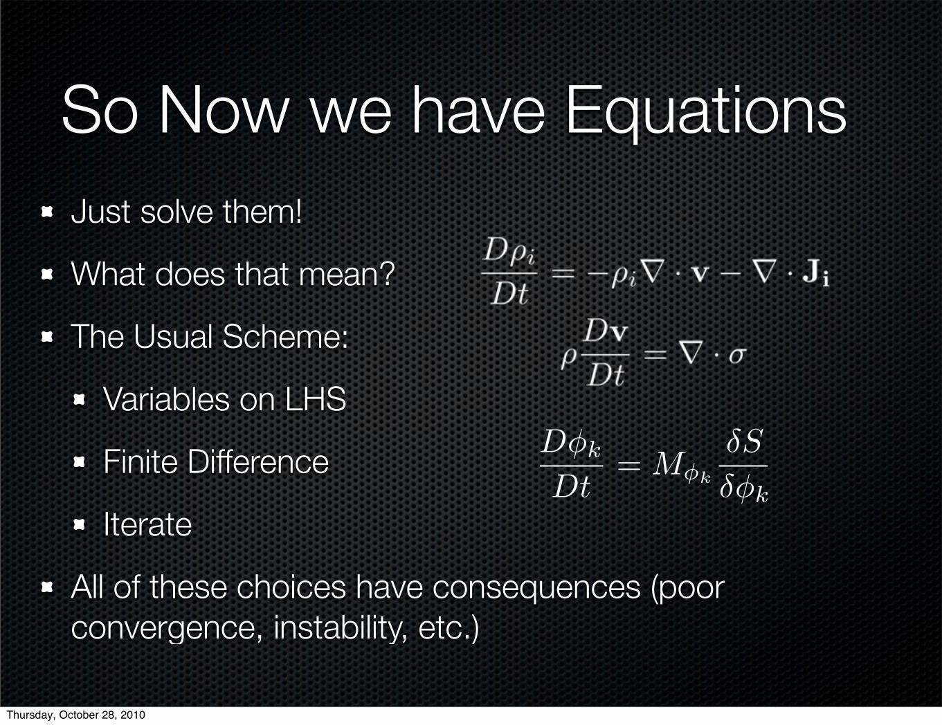
So Now we have EquationsJust solve them!
What does that mean?
The Usual Scheme:
Variables on LHS
Finite Difference
Iterate
All of these choices have consequences (poor convergence, instability, etc.)
Dφk
Dt= Mφk
δS
δφk
Thursday, October 28, 2010
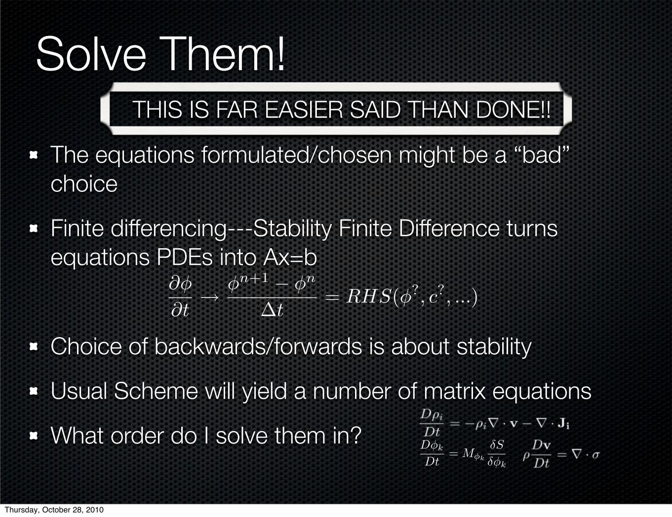
Solve Them!
The equations formulated/chosen might be a “bad” choice
Finite differencing---Stability Finite Difference turns equations PDEs into Ax=b
Choice of backwards/forwards is about stability
Usual Scheme will yield a number of matrix equations
What order do I solve them in?
∂φ
∂t→ φ
n+1 − φn
∆t= RHS(φ?
, c?, ...)
Dφk
Dt= Mφk
δS
δφk
THIS IS FAR EASIER SAID THAN DONE!!
Thursday, October 28, 2010
Outline
Motivation and Introduction Phase Field Method Thermodynamic derivation Numerical approach (FiPy digression) Results Conclusions
Thursday, October 28, 2010
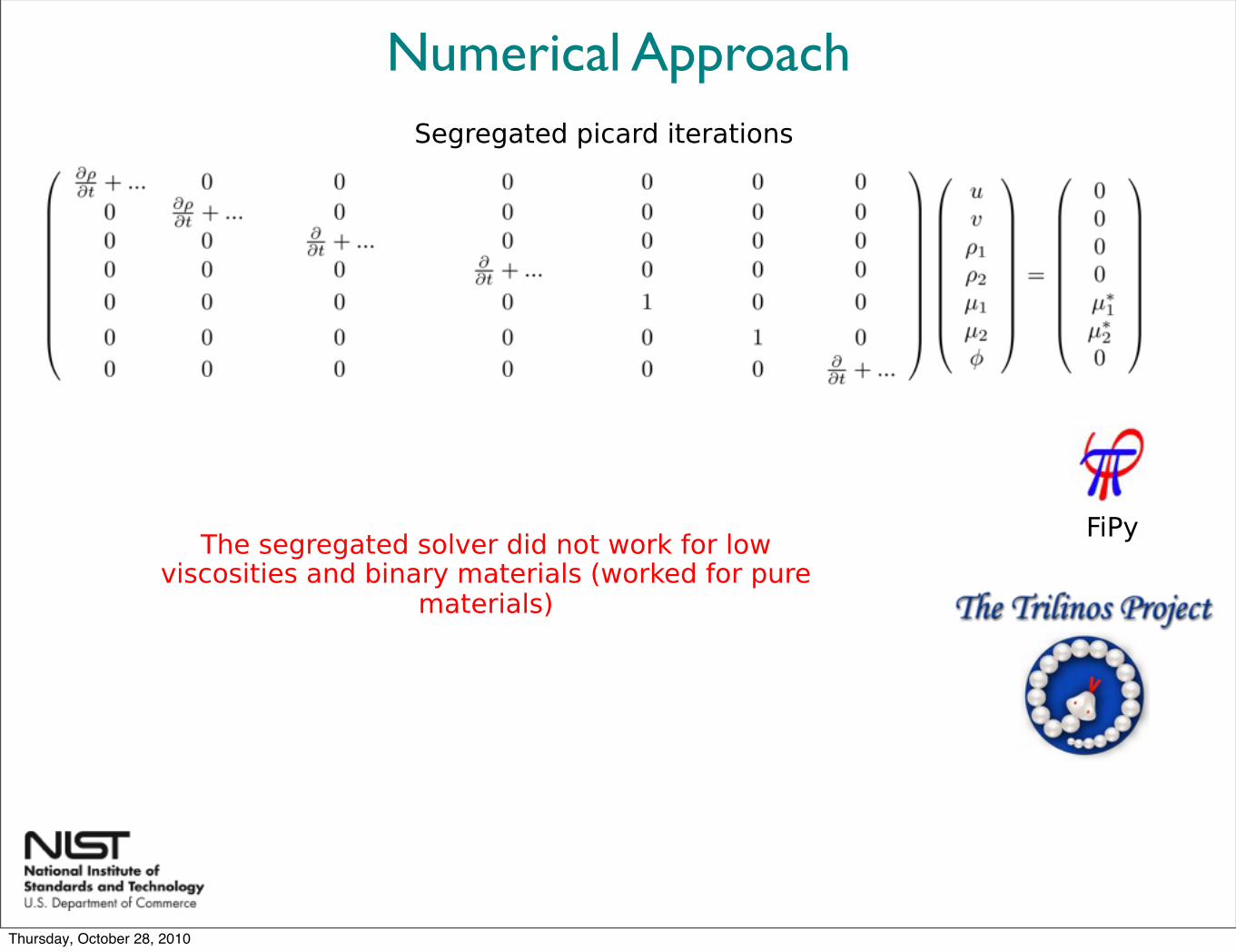
Numerical ApproachSegregated picard iterations
FiPyThe segregated solver did not work for low
viscosities and binary materials (worked for pure materials)
Thursday, October 28, 2010
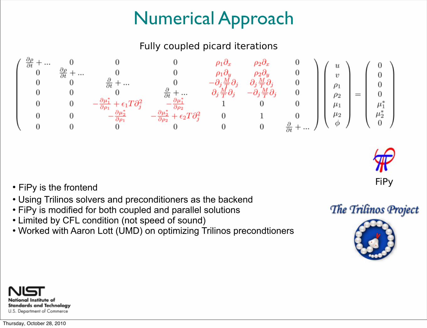
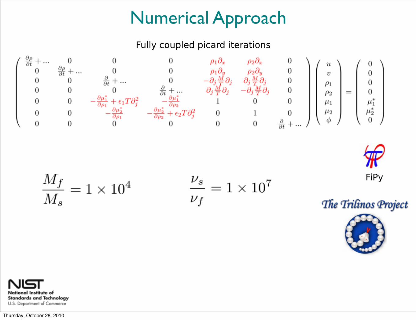
Numerical ApproachFully coupled picard iterations
FiPy is the frontend Using Trilinos solvers and preconditioners as the backend FiPy is modified for both coupled and parallel solutions Limited by CFL condition (not speed of sound) Worked with Aaron Lott (UMD) on optimizing Trilinos precondtioners
FiPy
Thursday, October 28, 2010
Numerical ApproachFully coupled picard iterations
FiPy
Thursday, October 28, 2010
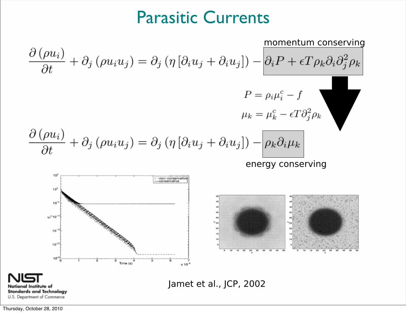
Parasitic Currents
Jamet et al., JCP, 2002
momentum conserving
energy conserving
Thursday, October 28, 2010
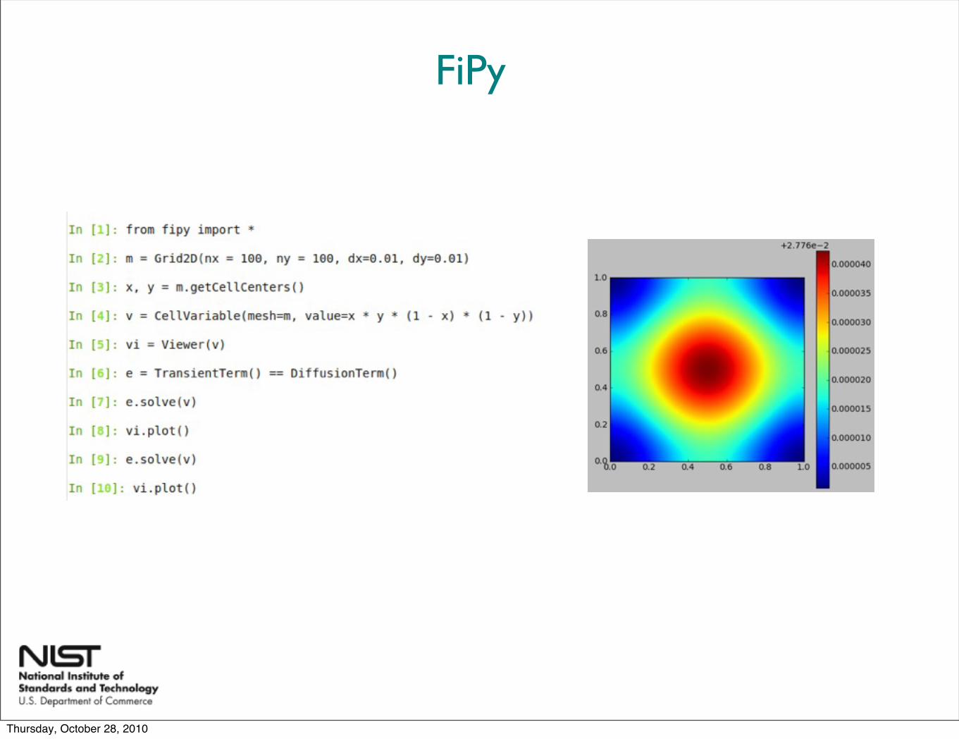
FiPy
Thursday, October 28, 2010
FiPy
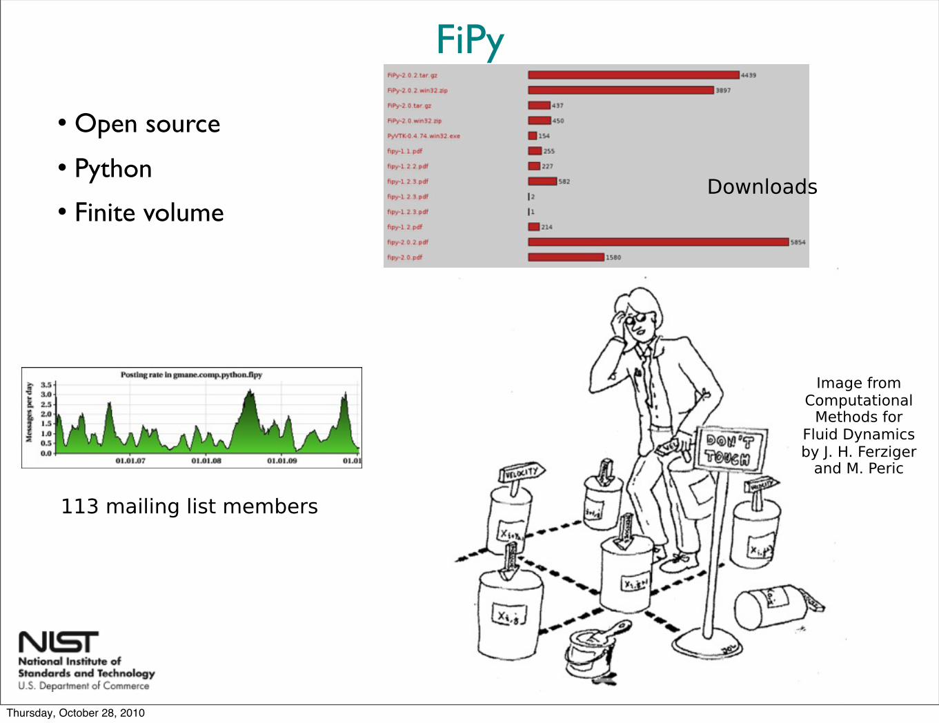
Open source Python Finite volume
113 mailing list members
Downloads
Image from Computational
Methods for Fluid Dynamics by J. H. Ferziger
and M. Peric
Thursday, October 28, 2010
Motivation and Introduction
Phase Field Method
Thermodynamic derivation
Numerical approach (FiPy digression)
Results
Conclusions
Thursday, October 28, 2010
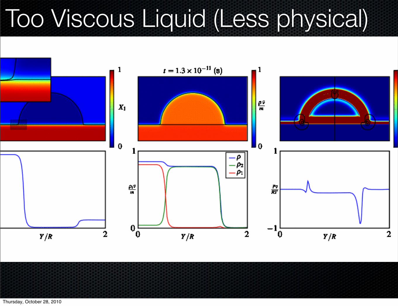
Too Viscous Liquid (Less physical)
Thursday, October 28, 2010
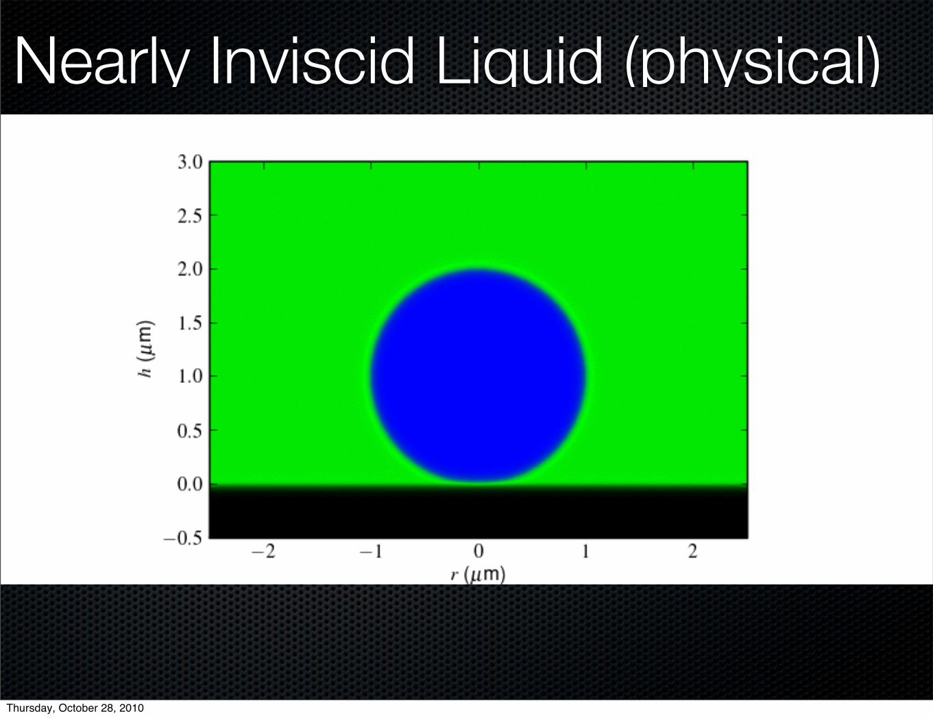
Nearly Inviscid Liquid (physical)
Thursday, October 28, 2010
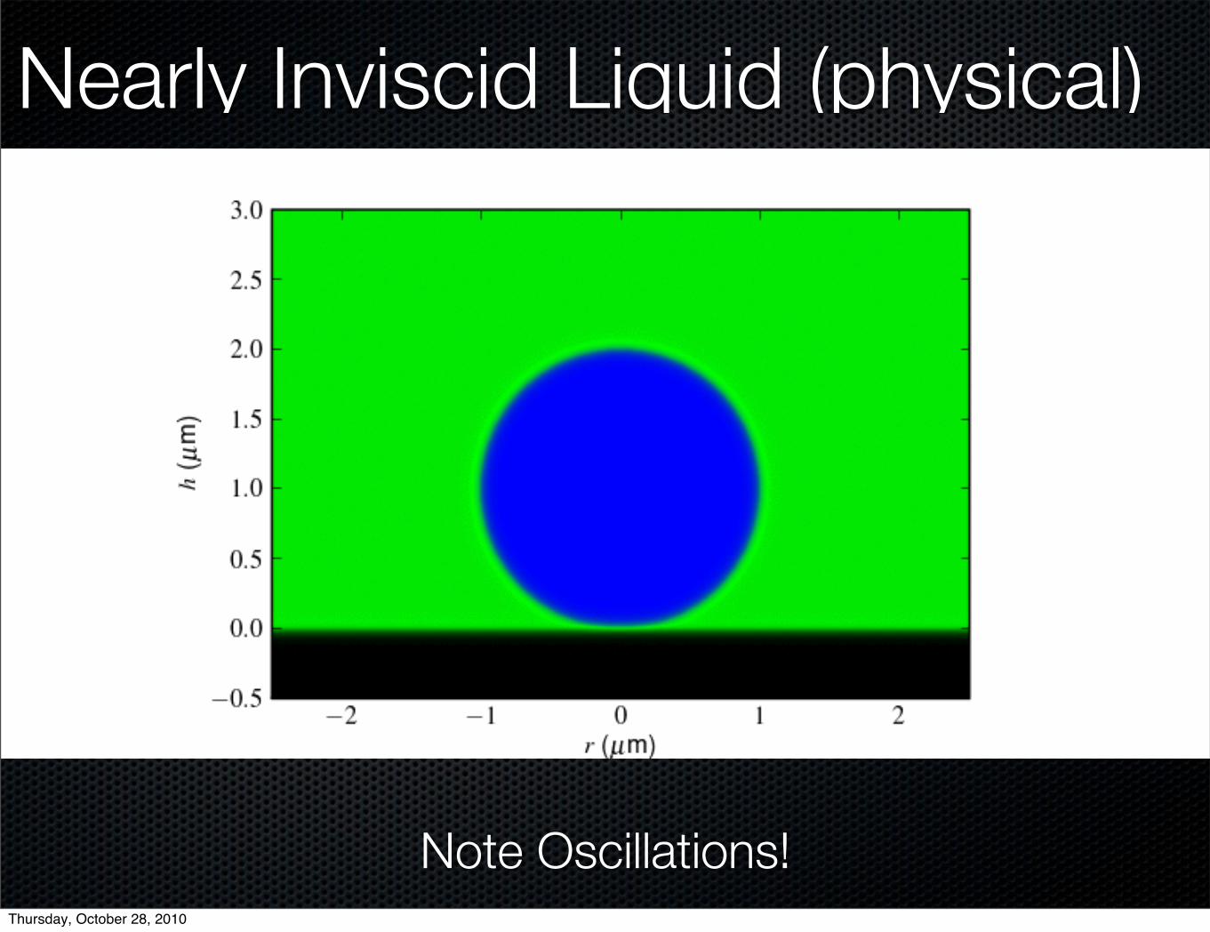
Nearly Inviscid Liquid (physical)
Note Oscillations!Thursday, October 28, 2010
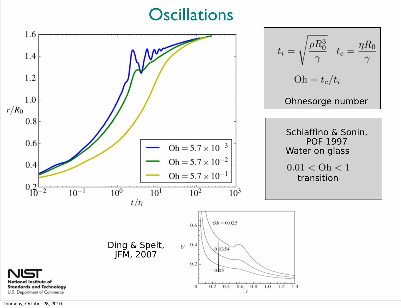
Oscillations
Ohnesorge number
Ding & Spelt, JFM, 2007
Water on glass
Schiaffino & Sonin, POF 1997
transition
Thursday, October 28, 2010
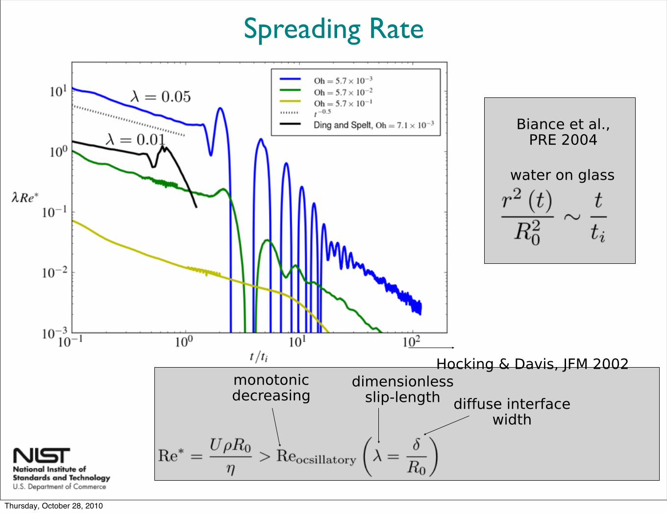
Spreading Rate
Biance et al.,PRE 2004
water on glass
Hocking & Davis, JFM 2002monotonic decreasing
dimensionless slip-length diffuse interface
width
Thursday, October 28, 2010
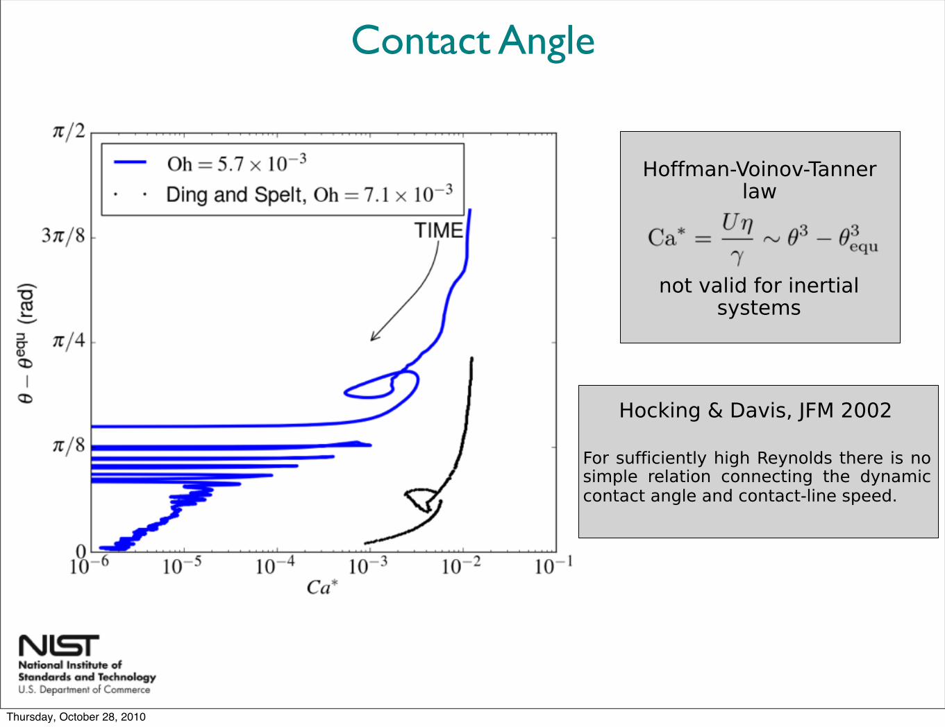
Contact Angle
Hoffman-Voinov-Tannerlaw
not valid for inertialsystems
Hocking & Davis, JFM 2002
For sufficiently high Reynolds there is no simple relation connecting the dynamic contact angle and contact-line speed.
Thursday, October 28, 2010
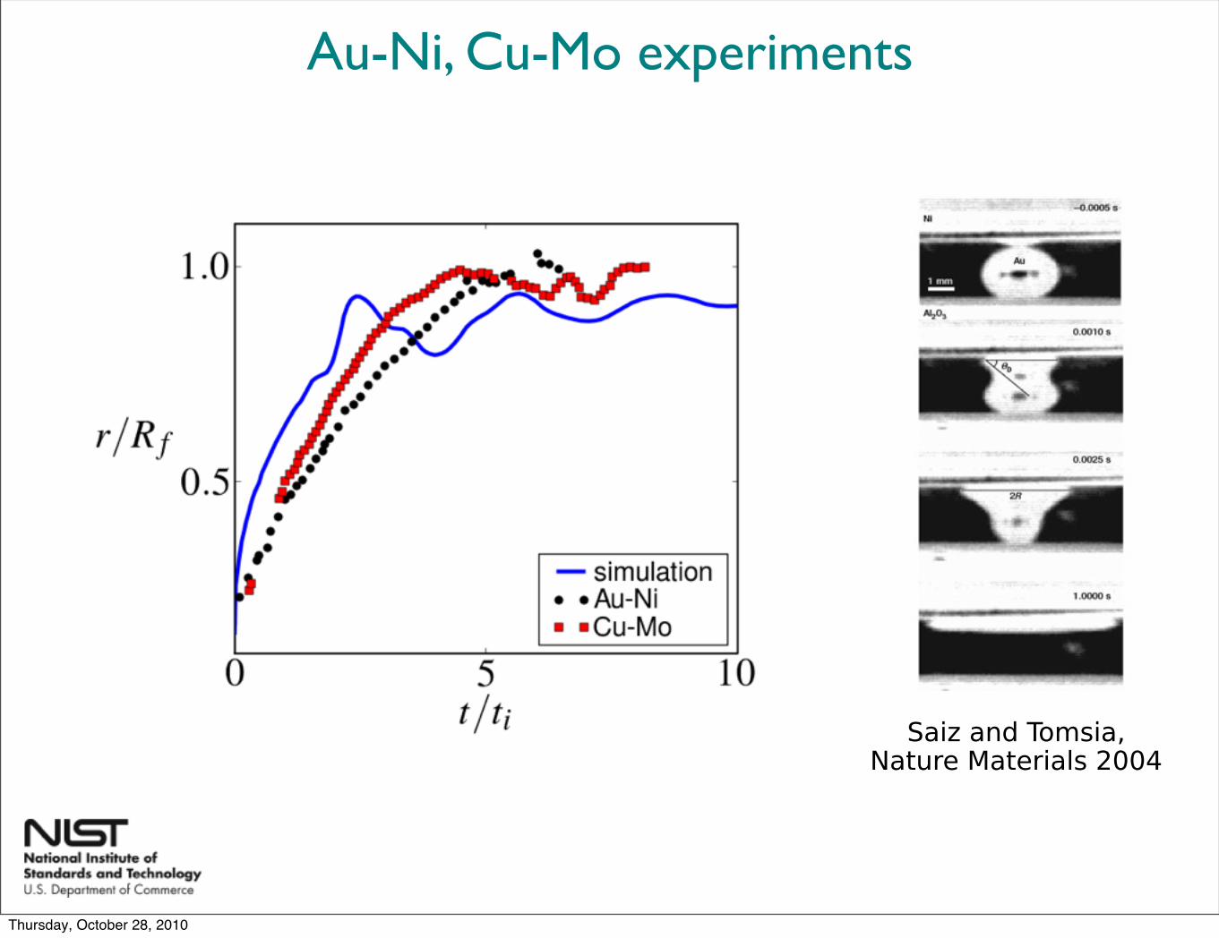
Au-Ni, Cu-Mo experiments
Saiz and Tomsia, Nature Materials 2004
Thursday, October 28, 2010
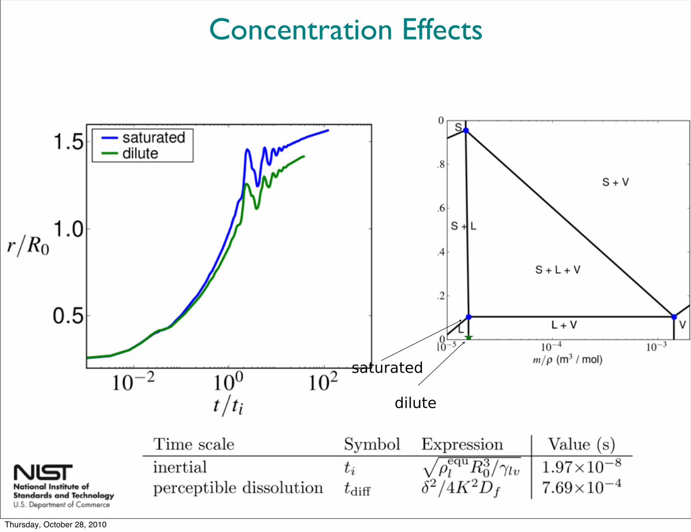
Concentration Effects
dilute
saturated
Thursday, October 28, 2010
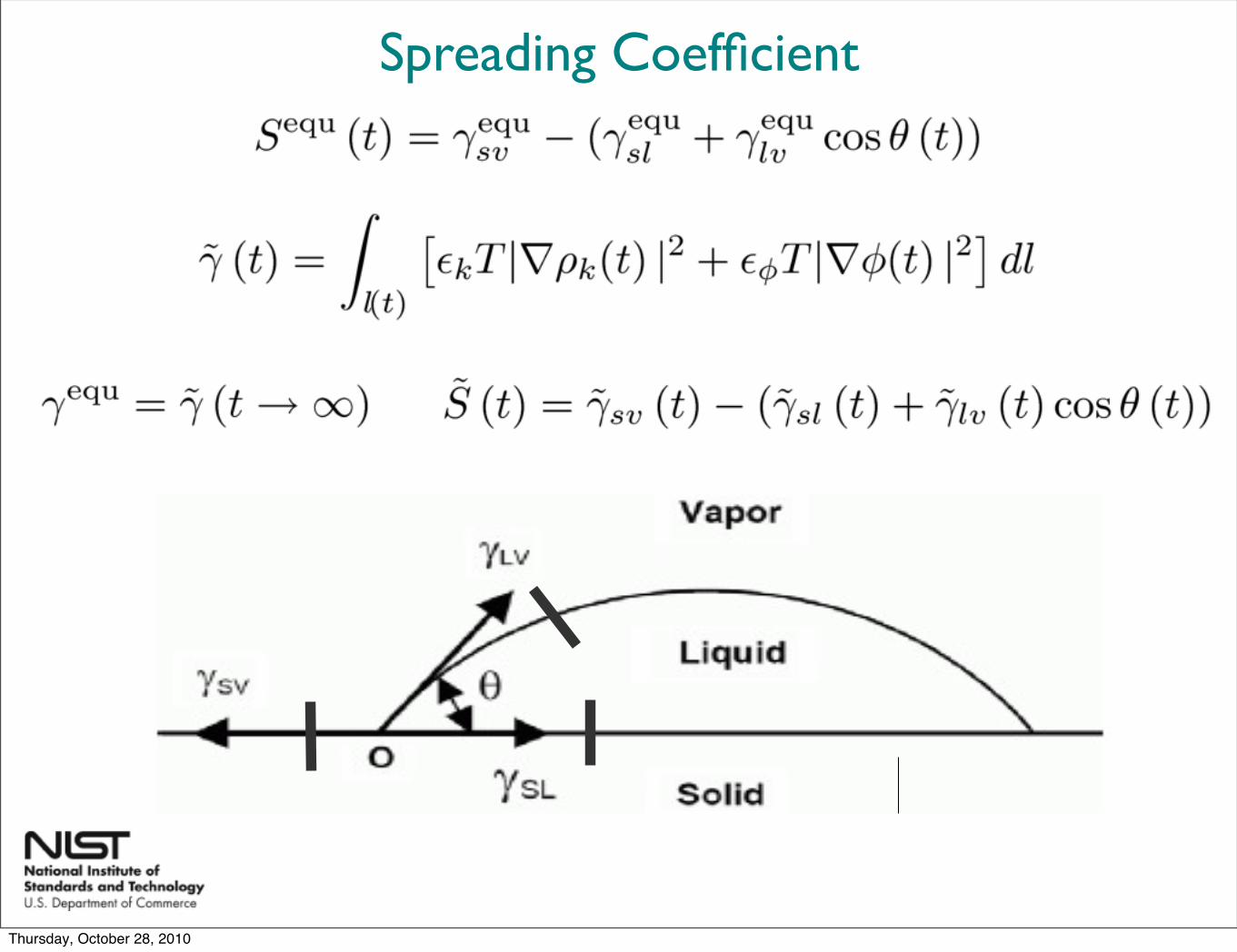
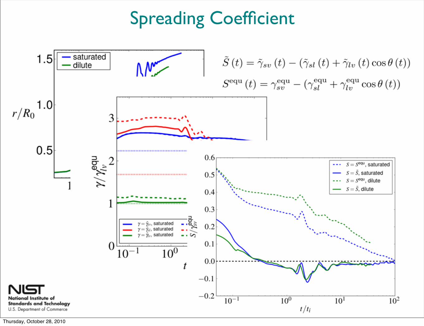
Spreading Coefficient
Thursday, October 28, 2010
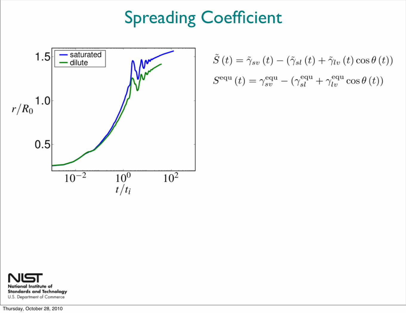
Spreading Coefficient
Thursday, October 28, 2010
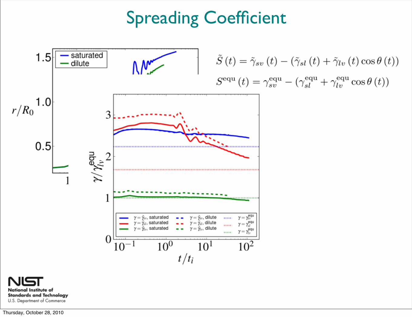
Spreading Coefficient
Thursday, October 28, 2010
Spreading Coefficient
Thursday, October 28, 2010
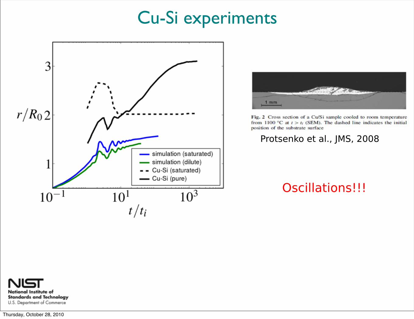
Cu-Si experiments
Protsenko et al., JMS, 2008
Oscillations!!!
Thursday, October 28, 2010
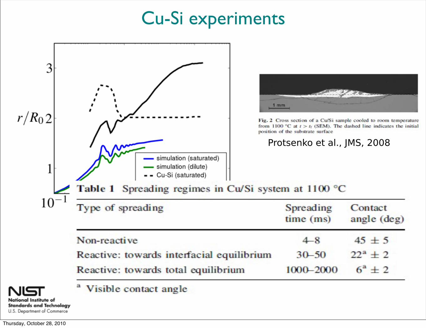
Cu-Si experiments
Protsenko et al., JMS, 2008
Oscillations!!!
Thursday, October 28, 2010
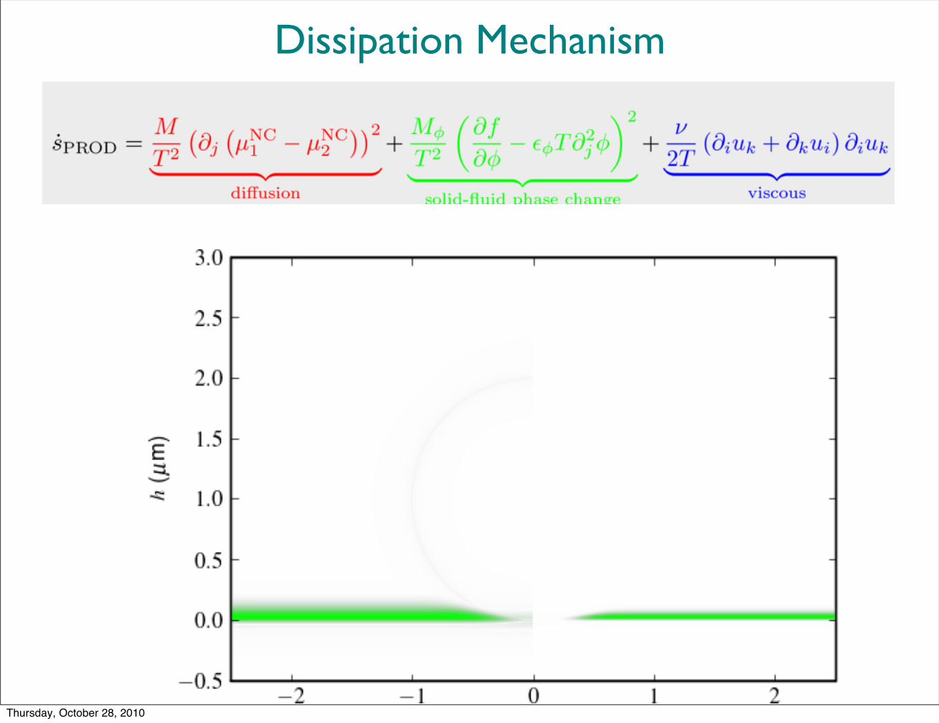
Dissipation Mechanism
Thursday, October 28, 2010

Thursday, October 28, 2010
Outline
Motivation and Introduction Thermodynamic derivation Numerical approach Results Conclusions
Thursday, October 28, 2010
Conclusions The dissipation mechanism is caused by “triple-line friction” when spreading is inertial. The dissipation mechanism is related to interface equilibration after inertial spreading. Larger drops, thinner interface, more physical Reactive wetting examples available soon with FiPy
Modeling the early stages of reactive wetting,Daniel Wheeler, James A. Warren and William J.
Boettinger,PRE (accepted for publication) 2010
Thursday, October 28, 2010