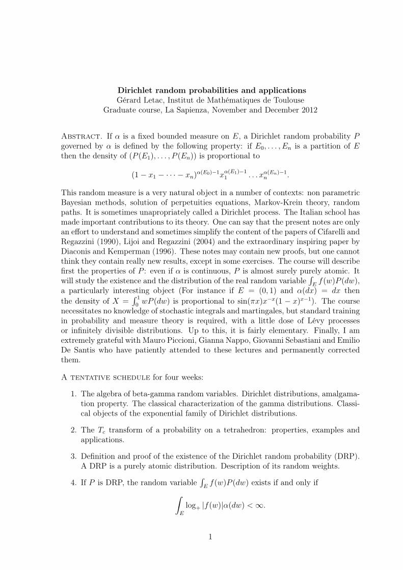
Dirichlet random probabilities and applications

Gérard Letac, Institut de Mathématiques de ToulouseGraduate course, La Sapienza, November and December 2012

Abstract. If α is a fixed bounded measure on E, a Dirichlet random probability Pgoverned by α is defined by the following property: if E0, . . . , En is a partition of Ethen the density of (P (E1), . . . , P (En)) is proportional to

(1− x1 − · · · − xn)α(E0)−1x

α(E1)−11 . . . xα(En)−1

n .

This random measure is a very natural object in a number of contexts: non parametricBayesian methods, solution of perpetuities equations, Markov-Krein theory, randompaths. It is sometimes unapropriately called a Dirichlet process. The Italian school hasmade important contributions to its theory. One can say that the present notes are onlyan effort to understand and sometimes simplify the content of the papers of Cifarelli andRegazzini (1990), Lijoi and Regazzini (2004) and the extraordinary inspiring paper byDiaconis and Kemperman (1996). These notes may contain new proofs, but one cannotthink they contain really new results, except in some exercises. The course will describefirst the properties of P : even if α is continuous, P is almost surely purely atomic. Itwill study the existence and the distribution of the real random variable

∫

Ef(w)P (dw),

a particularly interesting object (For instance if E = (0, 1) and α(dx) = dx then

the density of X =∫ 1

0wP (dw) is proportional to sin(πx)x−x(1 − x)x−1). The course

necessitates no knowledge of stochastic integrals and martingales, but standard trainingin probability and measure theory is required, with a little dose of Lévy processesor infinitely divisible distributions. Up to this, it is fairly elementary. Finally, I amextremely grateful with Mauro Piccioni, Gianna Nappo, Giovanni Sebastiani and EmilioDe Santis who have patiently attended to these lectures and permanently correctedthem.

A tentative schedule for four weeks:

1. The algebra of beta-gamma random variables. Dirichlet distributions, amalgama-tion property. The classical characterization of the gamma distributions. Classi-cal objects of the exponential family of Dirichlet distributions.

2. The Tc transform of a probability on a tetrahedron: properties, examples andapplications.

3. Definition and proof of the existence of the Dirichlet random probability (DRP).A DRP is a purely atomic distribution. Description of its random weights.

4. If P is DRP, the random variable∫

Ef(w)P (dw) exists if and only if

∫

E

log+ |f(w)|α(dw) < ∞.

1

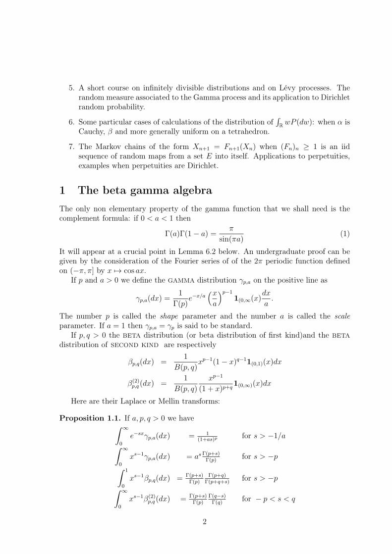
5. A short course on infinitely divisible distributions and on Lévy processes. Therandom measure associated to the Gamma process and its application to Dirichletrandom probability.

6. Some particular cases of calculations of the distribution of∫

RwP (dw): when α is

Cauchy, β and more generally uniform on a tetrahedron.

7. The Markov chains of the form Xn+1 = Fn+1(Xn) when (Fn)n ≥ 1 is an iidsequence of random maps from a set E into itself. Applications to perpetuities,examples when perpetuities are Dirichlet.

1 The beta gamma algebra

The only non elementary property of the gamma function that we shall need is thecomplement formula: if 0 < a < 1 then

Γ(a)Γ(1− a) =π

sin(πa)(1)

It will appear at a crucial point in Lemma 6.2 below. An undergraduate proof can begiven by the consideration of the Fourier series of of the 2π periodic function definedon (−π, π] by x 7→ cos ax.

If p and a > 0 we define the gamma distribution γp,a on the positive line as

γp,a(dx) =1

Γ(p)e−x/a

(x

a

)p−1

1(0,∞(x)dx

a.

The number p is called the shape parameter and the number a is called the scale

parameter. If a = 1 then γp,a = γp is said to be standard.If p, q > 0 the beta distribution (or beta distribution of first kind)and the beta

distribution of second kind are respectively

βp,q(dx) =1

B(p, q)xp−1(1− x)q−11(0,1)(x)dx

β(2)p,q (dx) =

1

B(p, q)

xp−1

(1 + x)p+q1(0,∞)(x)dx

Here are their Laplace or Mellin transforms:

Proposition 1.1. If a, p, q > 0 we have∫ ∞

0

e−sxγp,a(dx) = 1(1+as)p

for s > −1/a

∫ ∞

0

xs−1γp,a(dx) = as Γ(p+s)Γ(p)

for s > −p

∫ 1

0

xs−1βp,q(dx) = Γ(p+s)Γ(p)

Γ(p+q)Γ(p+q+s)

for s > −p

∫ ∞

0

xs−1β(2)p,q (dx) = Γ(p+s)

Γ(p)Γ(q−s)Γ(q)

for − p < s < q

2

The proof is obvious. Note that if Y ∼ γp,a then E( 1Y n ) = ∞ if n ≥ p.

Theorem 1.2. Let a, p, q > 0. If X ∼ γp,a and Y ∼ γq,a are independent, then the sum

S = X + Y ∼ γp+q,a is independent of U = XX+Y

∼ βp,q and V = XY∼ β

(2)p,q .

More generally, for n ≥ 2 and p1, . . . , pn > 0, consider the independent randomvariables X1, . . . , Xn such that Xk ∼ γpk,a for all k = 1, . . . , n. Define Sk = X1+· · ·+Xk

and qk = p1 + · · ·+ pk. Then

S1

S2

,S2

S3

, . . . ,Sn−1

Sn

, Sn

are independent random variables with Sk

Sk+1∼ βqk,pk+1

and Sn ∼ γqn,a.

Proof. For −p < t < q and s > −1/a the first part is proved by the followingcomputation:

E(

V te−sS)

= E

(

(

X

Y

)t

e−s(X+Y )

)

= E(

X te−sX)

E(

Y −te−sY)

=Γ(p+ t)

Γ(p)

Γ(q − t)

Γ(q)

1

(1 + as)p+q.

Note that U = XX+Y

∼ βp,q is implied by V = XY∼ β

(2)p,q .

We prove the second part by induction on n and things are more delicate. For n = 2this is the first part applied to X = X1, Y = X2, S = S2 and U = S1/S2. Assume thatthe statement is true for n ≥ 2 and let us prove it for n+1. By the induction hypothesis(Sn, Xn+1) is independent of S1

S2, S2

S3, . . . , Sn−1

Snand we use this fact when tk > −qk and

s > −1/a for writing that

E

(

(S1

S2

)t1(S2

S3

)t2 . . . (Sn−1

Sn

)tn−1(Sn

Sn+1

)tne−sSn+1

)

= E

(

(S1

S2

)t1(S2

S3

)t2 . . . (Sn−1

Sn

)tn−1

)

E

(

(Sn

Sn+1

)tne−sSn+1

)

=C

(1 + as)qn+1

n∏

k=1

Γ(qk + tk)

Γ(pk+1 + qk + tk)

where C is the constant with respect to t1, . . . , tn such that when t1 = . . . = tn = 0 thelast expression is 1.

Example 1: the chi square distribution with one degree of freedom. If Z ∼N(0, 1) then Z2 ∼ γ1/2,2 = χ2

1. To see this, compute the image of N(0, 1) by z 7→ y = z2

which is the composition of z 7→ u = |z| 7→ y = u2. We get

e−z2

2dz√2π

→ 2e−u2

2 1(0,∞)(u)du√2π

→ e−y2 y−1/2 dy

Γ(1/2).

Example 2: the chi square distribution with n degrees of freedom. IfZ1, . . . , Zn are independent random variables with the same distribution N(0, 1) then

Z21 + · · ·+ Z2

n ∼ γn/2,2 = χ2n

3

This comes from the above example for n = 1 and from Theorem 1.2.

Example 3: Gamma distribution and Brownian motion. Until recently, chisquare distributions were the only gamma distributions met in practical situations.Only in 1990 Dufresne (1990) and then Yor (1990) have shown that if B is a standardone dimensional Brownian motion then

(∫ ∞

0

eaB(t)−btdt

)−1

∼ γ 2ba2

,a2

2

(see Exercise 1.2). The important point of the remark is that the shape parameter 2ba2

is not necessarily a half integer.

We mention now a converse of the first part of Theorem 1.2. It is due to Lukacs (1956).

Theorem 1.3. Let X and Y be independent positive random variables not concen-trated on a single point such that S = X + Y and U = X/(X + Y ) are independent.Then there exist a, p, q > 0 such that X ∼ γp,a and Y ∼ γq,a.

Proof. For s > 0 denote LX(s) = E(e−sX) = e−kX(s). Therefore

−L′X(s)LY (s) = E(Xe−sX)E(e−sY ) = E(Xe−s(X+Y ))

= E(USe−sS) = E(U)E(Se−sS) = −E(U)L′S(s) = −E(U)(L′

X(s)LY (s) + LX(s)L′Y (s

As a consequence(1− E(U))k′

X(s) = E(U))k′Y (s).

Similarly

L′′X(s)LY (s) = E(X2e−sX)E(e−sY ) = E(X2e−s(X+Y ))

= E(U2S2e−sS) = E(U2)E(S2e−sS) = E(U2)L′′S(s)

= E(U2) (L′′X(s)LY (s) + 2L′

X(s)L′Y (s) + LX(s)L

′′Y (s)) .

leading to(k′

X)2 − k′′

X = E(U2)((k′X)

2 − k′′X + 2k′

Xk′Y + (k′

Y )2 − k′′

Y ) (2)

Denote for simplicity m1 = E(U), m2 = E(U2) and f(s) = m1k′Y (s). We get

k′X = f/(1−m1), k′

Y = f/m1.

Observe also that 0 < m21 < m2 < m1 < 1 : the point is that these inequalities are

strict from the hypothesis that X and Y are not concentrated on one point. With thesenotations, the equality (2) becomes the differential equation Af ′ + Bf 2 = 0 where

A =m1 −m2

m1(1−m1)> 0, B =

m2 −m21 + 2m1m2(1−m1)

m21(1−m1)2

> 0.

4

The solution of this differential equation is f(s) = A/(C + Bs) where C is an ar-bitrary constant which must be > 0 since k′

Y (s) > 0 on s > 0. As a consequencekY (s) = m1

ABlog(1 + B

Cs) (the constant of integration is determined by lims→0 kY (s) =

0). Therefore

LY (s) =1

(1 + as)q

is the Laplace transform of γq,a with q = m1A/B and a = B/C. The reasoning for LX

is plain.

Exercice 1.1. If S ∼ γp+q,a and U ∼ βp,q are independent, show that SU ∼ γp,a (Hint:use the Mellin transform of SU and Proposition 1.1)

Exercice 1.2. If Z ∼ N(0, t) compute E(eaZ). Use the result for computing f(a, b) =E(Y (a, b)) where Y (a, b) =

∫∞

0eaB(t)−btdt , where B is a standard Brownian motion and

where b > a2/2 > 0. Show that if b > n|a|/2 then E(Y n(a, b)) = n!∏n

k=1 f(ka, kb). Hintfor n = 2:

E(Y 2(a, b)) = 2E

(∫

0<t1<t2

e2aB(t1)+a(B(t2)−B(t1))−2bt1−b(t2−t1)dt1dt2

)

= 2E

(∫ ∞

0

e2aB(t1)−2bt1dt1 ×∫ ∞

0

eaB2(s2)−bs2ds2

)

by introducing for fixed t1 the Brownian motion B2(s2) = B(t1 + s2) − B(t1) which isindependent of B(t1). Finally prove that E(Y n(a, b)) =

∫∞

0x−nγ 2b

a2,a

2

2

(dx). What are the

values on n such that E(Y n(a, b)) is finite? Note that this calculation does not provecompletely that Y −1(a, b) ∼ γ 2b

a2,a

2

2

since we have only proved that a finite number of

moments coincide.

2 The Dirichlet distribution

We will need the following notation. The natural basis of Rd+1 is denoted by e0, . . . ed.The convex hull of e0, . . . ed is a tetrahedron that we denote by Ed+1. The elements ofEd+1 are therefore the vectors λ = (λ0, . . . , λd) of Rd+1 such that λi ≥ 0 for i = 0, . . . , dand such that λ0 + · · ·+ λd = 1. If a0, . . . , ad are positive numbers the Dirichlet distri-bution D(a0, . . . , ad) of X = (X0, . . . , Xd) ∈ Ed+1 is such that the law of (X1, . . . , Xd)is

1

B(a0, . . . , ad)(1− x1 − · · · − xd)

a0−1xa1−11 . . . xad−1

d 1Td(x1, . . . , xd)dx1, . . . dxd (3)

where B(a0, . . . , ad) =Γ(a0)...Γ(ad)Γ(a0+...+ad)

and where Td is the set of (x1, . . . , xd) such that xi > 0for all i = 0, 1, . . . , d, with the convention x0 = 1− x1 · · · − xd. For instance, if the realrandom variable X1 follows the beta distribution

β(a1, a0)(dx) =1

B(a1, a0)xa1−1(1− x)a0−11(0,1)(x)dx

5

then (X1, 1−X1) ∼ D(a1, a0). A simple example is D(a0, . . . , ad), which is the uniformprobability on the tetrahedron Ed+1). It is not clear that (3) has total mass 1, thenext theorem will show it. Indeed, the following result is crucial for the Dirichletdistributions:

Theorem 2.1. Consider the independent random variables X0, . . . , Xd such that Xk ∼γak,c for all k = 0, . . . , d and define S = X0+· · ·+Xd. Then S is independent of the vector1S(X0, . . . , Xd). Furthermore 1

S(X1, . . . , Xd) has the density (3) and 1

S(X0, . . . , Xd) ∼

D(a0, . . . , ad).

Proof. Denote a = a0 + · · ·+ ad. It seems that the method of the Jacobian is after allthe quickest. We look for the image of the probability

e−1

c(x0+···+xd)xa0−1

0 xa1−11 . . . xad−1

d

1

ca∏d

k=0 Γ(ak)1(0,∞)d+1(x0, . . . , xn)dx0 . . . dxn

by the map(x0, . . . , xn) 7→ (y1, . . . , yd, s) (4)

defined by s = x0 + · · ·+ xd and yi = xi/s with i = 1, . . . , d. The inverse is given by

x1 = sy1, . . . , xd = syd, x0 = s(1− y1 − · · · − yd) = sy0

and the Jacobian matrix is very easy to compute

s 0 0 . . . 0 y10 s 0 . . . 0 y2. . . . . . . . . . . . . . . . . .0 0 0 . . . s yd−s −s −s . . . −s y0

Adding the first d rows to the last one shows easily that its determinant is sd and theimage of the probability (4) is

e−sc

sa−1

ca−1Γ(a)1(0,∞(s)ds× 1

B(a0, . . . , ad)(1−y1−· · ·−yd)

a0−1ya1−11 . . . yad−1

d 1Td(y1, . . . , yd)dy1 . . . dyd

where Td = (y1, . . . , yd); yi > 0, i = 0, 1, . . . , n (recall the notation y0 = 1−y1−· · ·−yd)

Remarks: Let us insist on the fact that the Dirichlet distribution D(a0, . . . , ad) isa singular distribution in R

d+1 concentrated on the tetraedron Ed+1 However, manycalculations about it can only be performed by using the density of its projection(x0, . . . , xd) 7→ (x1, . . . , xd) from Ed+1 to Td.

For the next proposition we use the Pochhammer symbol (X)n = X(X + 1)(X +2) . . . (X + n− 1) for n > 0 with the convention (X)0 = 1.

6

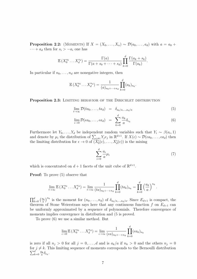
Proposition 2.2: (Moments) If X = (X0, . . . , Xn) ∼ D(a0, . . . , ad) with a = a0 +· · ·+ ad then for si > −ai one has

E (Xs00 . . . Xsd

d ) =Γ(a)

Γ(a+ s0 + · · ·+ sd)

d∏

k=0

Γ(ak + sk)

Γ(ak).

In particular if n0, . . . , nd are nonegative integers, then

E (Xn0

0 . . . Xndd ) =

1

(a)n0+···+nd

d∏

k=0

(ak)nk.

Proposition 2.3: Limiting behavior of the Dirichlet distribution

limt→∞

D(ta0, . . . , tad) = δa0/a,...,ad/a (5)

limε→0

D(εa0, . . . , εad) =d∑

k=0

akaδek (6)

Furthermore let Y0, . . . , Yd be independent random variables such that Yi ∼ β(ai, 1)and denote by µi the distribution of

∑

j 6=i Yjej in Rd+1. If X(ε) ∼ D(εa0, . . . , εad) then

the limiting distribution for ε → 0 of (Xε0(ε), . . . , X

εd(ε)) is the mixing

d∑

i=0

aiaµi (7)

which is concentrated on d+ 1 facets of the unit cube of Rd+1.

Proof: To prove (5) observe that

limt→∞

E (Xn0

0 . . . Xndd ) = lim

t→∞

1

(ta)n0+···+nd

d∏

k=0

(tak)nk=

d∏

k=0

(aka

)nk

.

∏dk=0

(

aka

)nk is the moment for (n0, . . . , nd) of δa0/a,...,ad/a. Since Ed+1 is compact, thetheorem of Stone Weierstrass says here that any continuous function f on Ed+1 canbe uniformly approximated by a sequence of polynomials. Therefore convergence ofmoments implies convergence in distribution and (5 is proved.

To prove (6) we use a similar method. But

limε→0

E (Xn0

0 . . . Xndd ) = lim

ε→∞

1

(εa)n0+···+nd

d∏

k=0

(εak)nk

is zero if all nj > 0 for all j = 0, . . . , d and is ak/a if nk > 0 and the others nj = 0for j 6= k. This limiting sequence of moments corresponds to the Bernoulli distribution∑d

k=0akaδek .

7

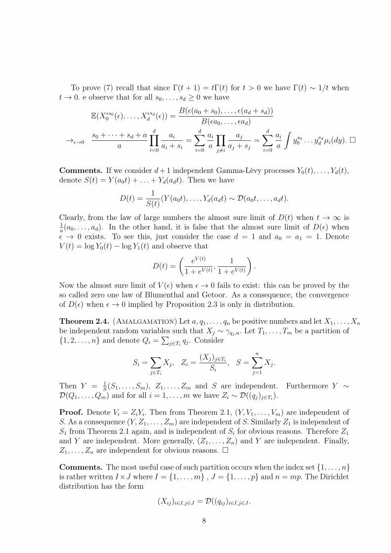
To prove (7) recall that since Γ(t + 1) = tΓ(t) for t > 0 we have Γ(t) ∼ 1/t whent → 0. e observe that for all s0, . . . , sd ≥ 0 we have

E(Xεs00 (ε), . . . , Xεsd

d (ε)) =B(ε(a0 + s0), . . . , ε(ad + sd))

B(εa0, . . . , εad)

→ε→0s0 + · · ·+ sd + a

a

d∏

i=0

aiai + si

=d∑

i=0

aia

∏

j 6=i

ajaj + sj

=d∑

i=0

aia

∫

ys00 . . . ysdd µi(dy).

Comments. If we consider d+1 independent Gamma-Lévy processes Y0(t), . . . , Yd(t),denote S(t) = Y (a0t) + . . .+ Yd(adt). Then we have

D(t) =1

S(t)(Y (a0t), . . . , Yd(adt) ∼ D(a0t, . . . , adt).

Clearly, from the law of large numbers the almost sure limit of D(t) when t → ∞ is1a(a0, . . . , ad). In the other hand, it is false that the almost sure limit of D(ε) when

ε → 0 exists. To see this, just consider the case d = 1 and a0 = a1 = 1. DenoteV (t) = log Y0(t)− log Y1(t) and observe that

D(t) =

(

eV (t)

1 + eV (t),

1

1 + eV (t)

)

.

Now the almost sure limit of V (ε) when ε → 0 fails to exist: this can be proved by theso called zero one law of Blumenthal and Getoor. As a consequence, the convergenceof D(ε) when ε → 0 implied by Proposition 2.3 is only in distribution.

Theorem 2.4. (Amalgamation) Let a, q1, . . . , qn be positive numbers and let X1, . . . , Xn

be independent random variables such that Xj ∼ γqj ,a. Let T1, . . . , Tm be a partition of1, 2, . . . , n and denote Qi =

∑

j∈Tiqj. Consider

Si =∑

j∈Ti

Xj, Zi =(Xj)j∈Ti

Si

, S =n∑

j=1

Xj.

Then Y = 1S(S1, . . . , Sm), Z1, . . . , Zm and S are independent. Furthermore Y ∼

D(Q1, . . . , Qm) and for all i = 1, . . . ,m we have Zi ∼ D((qj)j∈Ti).

Proof. Denote Vi = ZiYi. Then from Theorem 2.1, (Y, V1, . . . , Vm) are independent ofS. As a consequence (Y, Z1, . . . , Zm) are independent of S. Similarly Z1 is independent ofS1 from Theorem 2.1 again, and is independent of Si for obvious reasons. Therefore Z1

and Y are independent. More generally, (Z1, . . . , Zn) and Y are independent. Finally,Z1, . . . , Zn are independent for obvious reasons.

Comments. The most useful case of such partition occurs when the index set 1, . . . , nis rather written I×J where I = 1, . . . ,m , J = 1, . . . , p and n = mp. The Dirichletdistribution has the form

(Xij)i∈I,j∈J = D((qij)i∈I,j∈J .

8

If we consider the partition Ti = i× J and Qi =∑m

j=1 qij and Xi. =∑m

j=1 Xij we get

(X1., . . . , Xm.) ∼ D(Q1, . . . , Qm).

(see exercise 2.4)

Corollary 2.5. Let q1, . . . , qn be positive numbers. Let T1, . . . , Tm be a partition of1, 2, . . . , n and denote Qi =

∑

j∈Tiqj. If X ∼ D(q1, . . . , qn) and if Yi =

∑

j∈TiXj then

(Y1, . . . , Ym) ∼ D(Q1, . . . , Qm).

In particular Xj ∼ βqj ,Q−qj if Q =∑d

i=0 qi.

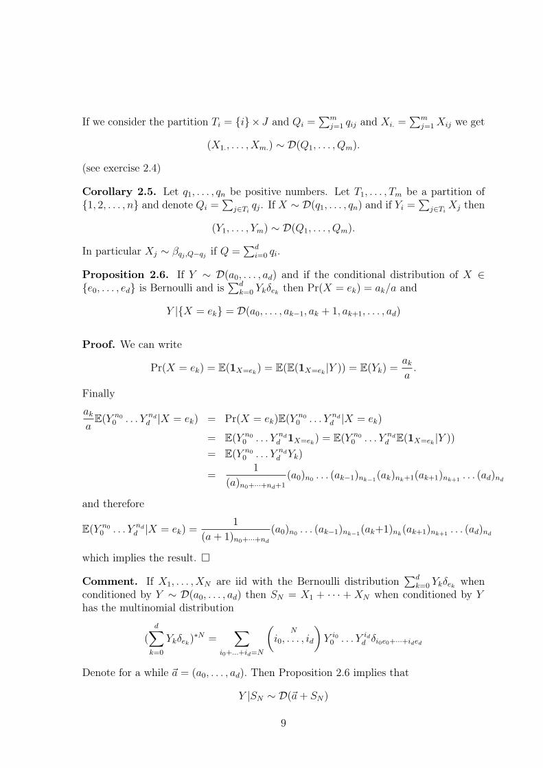
Proposition 2.6. If Y ∼ D(a0, . . . , ad) and if the conditional distribution of X ∈e0, . . . , ed is Bernoulli and is

∑dk=0 Ykδek then Pr(X = ek) = ak/a and

Y |X = ek = D(a0, . . . , ak−1, ak + 1, ak+1, . . . , ad)

Proof. We can write

Pr(X = ek) = E(1X=ek) = E(E(1X=ek |Y )) = E(Yk) =aka.

Finally

akaE(Y n0

0 . . . Y ndd |X = ek) = Pr(X = ek)E(Y

n0

0 . . . Y ndd |X = ek)

= E(Y n0

0 . . . Y ndd 1X=ek) = E(Y n0

0 . . . Y ndd E(1X=ek |Y ))

= E(Y n0

0 . . . Y ndd Yk)

=1

(a)n0+···+nd+1

(a0)n0. . . (ak−1)nk−1

(ak)nk+1(ak+1)nk+1. . . (ad)nd

and therefore

E(Y n0

0 . . . Y ndd |X = ek) =

1

(a+ 1)n0+···+nd

(a0)n0. . . (ak−1)nk−1

(ak+1)nk(ak+1)nk+1

. . . (ad)nd

which implies the result.

Comment. If X1, . . . , XN are iid with the Bernoulli distribution∑d

k=0 Ykδek whenconditioned by Y ∼ D(a0, . . . , ad) then SN = X1 + · · · + XN when conditioned by Yhas the multinomial distribution

(d∑

k=0

Ykδek)∗N =

∑

i0+...+id=N

(

N

i0, . . . , id

)

Y i00 . . . Y id

d δi0e0+···+ided

Denote for a while ~a = (a0, . . . , ad). Then Proposition 2.6 implies that

Y |SN ∼ D(~a+ SN)

9

as can be seen by induction on N.

The next proposition shows that a Dirichlet distribution can generates a non homoge-

neous Markov chain:

Proposition 2.7. (Y1, . . . , Yn) ∼ D(p1, . . . , pn) and if Fk = Y1 + · · ·+ Yk then (Fk)nk=0

is a Markov chain. Its transition kernel is such that for 1 ≤ k ≤ n − 1 we haveFk|Fk−1 = (1− Fk−1)Bk where

Bk ∼ βpk,pk+1+···+pn .

Proof. We start from the independent random variables X1, . . . , Xn such that Xk ∼γpk,a for all k = 1, . . . , n. Defining Sk = X1 + · · ·+Xk and qk = p1 + · · ·+ pk.

Theorem 1.2 says thatS1

S2

,S2

S3

, . . . ,Sn−1

Sn

, Sn

are independent random variables with Sk

Sk+1∼ βqk,pk+1

and Sn ∼ γqn,a. Denoting Yi =

Xi/Sn we get thatF1

F2

,F2

F3

, . . . ,Fn−1

Fn

= Fn−1, Sn

are independent.

The next two propositions give two useful geometrical examples of Dirichlet distribu-tions

Proposition 2.7: (Uniform distribution on the Euclidean sphere) If E = Rn

has its natural Euclidean structure, let S be the unit sphere of E and denote by µ(ds)the uniform measure on S namely the unique measure on S which is invariant by allorthogonal transformations s 7→ u(s) where u is in the orthogonal group O(E). LetZ = (Z1, . . . , Zn) ∼ N(0, In) be a standard Gaussian variable in E. Then

Θ = (Θ1, . . . ,Θn) =Z

‖Z‖

is uniform and (Θ21, . . . ,Θ

2n) ∼ D(1/2, . . . , 1/2)

Proposition 2.8: (Uniform distribution on the Hermitian sphere) If H = Cn

has its natural Hermitian structure, let S be the unit sphere of H and denote byµ(ds) the uniform measure on S namely the unique measure on S which is invariantby all unitary transformations s 7→ u(s) where u is in the unitary group U(H). LetZ = (Z1, . . . , Zn) ∼ N(0, In) be a standard Gaussian variable in E. Then

Θ = (Θ1, . . . ,Θn) =Z

‖Z‖

is uniform and (‖Θ1‖2, . . . , ‖Θn‖2) ∼ D(1, . . . , 1) is uniform in the tetrahedron En.

10

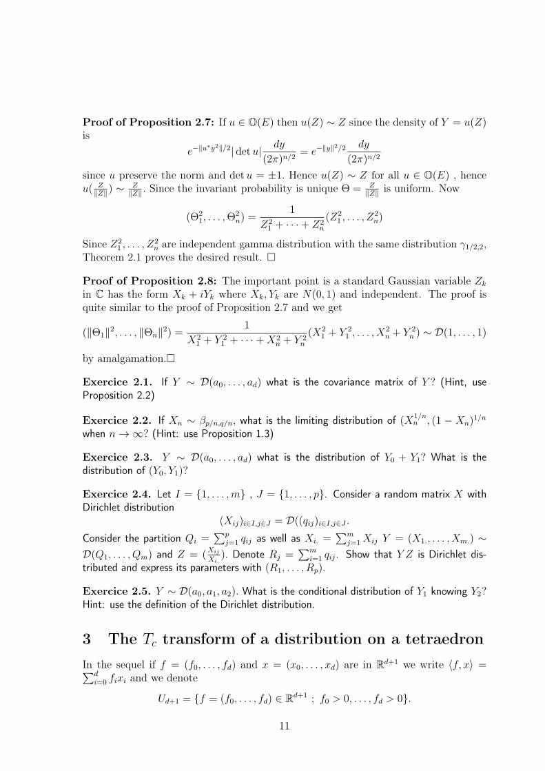
Proof of Proposition 2.7: If u ∈ O(E) then u(Z) ∼ Z since the density of Y = u(Z)is

e−‖u∗y2‖/2| det u| dy

(2π)n/2= e−‖y‖2/2 dy

(2π)n/2

since u preserve the norm and det u = ±1. Hence u(Z) ∼ Z for all u ∈ O(E) , henceu( Z

‖Z‖) ∼ Z

‖Z‖. Since the invariant probability is unique Θ = Z

‖Z‖is uniform. Now

(Θ21, . . . ,Θ

2n) =

1

Z21 + · · ·+ Z2

n

(Z21 , . . . , Z

2n)

Since Z21 , . . . , Z

2n are independent gamma distribution with the same distribution γ1/2,2,

Theorem 2.1 proves the desired result.

Proof of Proposition 2.8: The important point is a standard Gaussian variable Zk

in C has the form Xk + iYk where Xk, Yk are N(0, 1) and independent. The proof isquite similar to the proof of Proposition 2.7 and we get

(‖Θ1‖2, . . . , ‖Θn‖2) =1

X21 + Y 2

1 + · · ·+X2n + Y 2

n

(X21 + Y 2

1 , . . . , X2n + Y 2

n ) ∼ D(1, . . . , 1)

by amalgamation.

Exercice 2.1. If Y ∼ D(a0, . . . , ad) what is the covariance matrix of Y ? (Hint, useProposition 2.2)

Exercice 2.2. If Xn ∼ βp/n,q/n, what is the limiting distribution of (X1/nn , (1 − Xn)

1/n

when n → ∞? (Hint: use Proposition 1.3)

Exercice 2.3. Y ∼ D(a0, . . . , ad) what is the distribution of Y0 + Y1? What is thedistribution of (Y0, Y1)?

Exercice 2.4. Let I = 1, . . . ,m , J = 1, . . . , p. Consider a random matrix X withDirichlet distribution

(Xij)i∈I,j∈J = D((qij)i∈I,j∈J .

Consider the partition Qi =∑p

j=1 qij as well as Xi. =∑m

j=1 Xij Y = (X1., . . . , Xm.) ∼D(Q1, . . . , Qm) and Z = (

Xij

Xi.). Denote Rj =

∑mi=1 qij. Show that Y Z is Dirichlet dis-

tributed and express its parameters with (R1, . . . , Rp).

Exercice 2.5. Y ∼ D(a0, a1, a2). What is the conditional distribution of Y1 knowing Y2?Hint: use the definition of the Dirichlet distribution.

3 The Tc transform of a distribution on a tetraedron

In the sequel if f = (f0, . . . , fd) and x = (x0, . . . , xd) are in Rd+1 we write 〈f, x〉 =

∑di=0 fixi and we denote

Ud+1 = f = (f0, . . . , fd) ∈ Rd+1 ; f0 > 0, . . . , fd > 0.

11

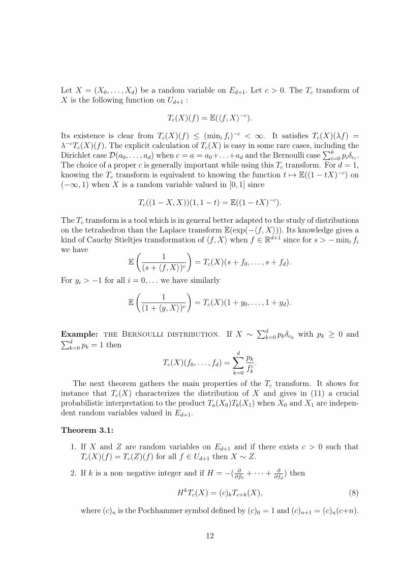
Let X = (X0, . . . , Xd) be a random variable on Ed+1. Let c > 0. The Tc transform ofX is the following function on Ud+1 :

Tc(X)(f) = E(〈f,X〉−c).

Its existence is clear from Tc(X)(f) ≤ (mini fi)−c < ∞. It satisfies Tc(X)(λf) =

λ−cTc(X)(f). The explicit calculation of Tc(X) is easy in some rare cases, including theDirichlet case D(a0, . . . , ad) when c = a = a0+. . .+ad and the Bernoulli case

∑ki=0 piδei .

The choice of a proper c is generally important while using this Tc transform. For d = 1,knowing the Tc transform is equivalent to knowing the function t 7→ E((1− tX)−c) on(−∞, 1) when X is a random variable valued in [0, 1] since

Tc((1−X,X))(1, 1− t) = E((1− tX)−c).

The Tc transform is a tool which is in general better adapted to the study of distributionson the tetrahedron than the Laplace transform E(exp(−〈f,X〉)). Its knowledge gives akind of Cauchy Stieltjes transformation of 〈f,X〉 when f ∈ R

d+1 since for s > −mini fiwe have

E

(

1

(s+ 〈f,X〉)c)

= Tc(X)(s+ f0, . . . , s+ fd).

For yi > −1 for all i = 0, . . . we have similarly

E

(

1

(1 + 〈y,X〉)c)

= Tc(X)(1 + y0, . . . , 1 + yd).

Example: the Bernoulli distribution. If X ∼ ∑dk=0 pkδek with pk ≥ 0 and

∑dk=0 pk = 1 then

Tc(X)(f0, . . . , fd) =d∑

k=0

pkf ck

.

The next theorem gathers the main properties of the Tc transform. It shows forinstance that Tc(X) characterizes the distribution of X and gives in (11) a crucialprobabilistic interpretation to the product Ta(X0)Tb(X1) when X0 and X1 are indepen-dent random variables valued in Ed+1.

Theorem 3.1:

1. If X and Z are random variables on Ed+1 and if there exists c > 0 such thatTc(X)(f) = Tc(Z)(f) for all f ∈ Ud+1 then X ∼ Z.

2. If k is a non–negative integer and if H = −( ∂∂f0

+ · · ·+ ∂∂fd

) then

HkTc(X) = (c)kTc+k(X), (8)

where (c)n is the Pochhammer symbol defined by (c)0 = 1 and (c)n+1 = (c)n(c+n).

12

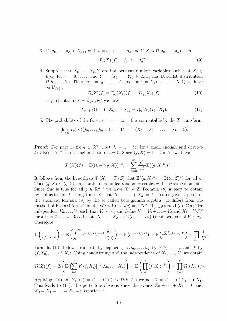
3. If (a0, . . . , ad) ∈ Ud+1 with a = a0 + . . .+ ad and if X ∼ D(a0, . . . , ad) then

Ta(X)(f) = f−a00 . . . f−ad

d . (9)

4. Suppose that X0, . . . , Xr, Y are independent random variables such that Xi ∈Ed+1 for i = 0, . . . , r and Y = (Y0, . . . , Yr) ∈ Er+1 has Dirichlet distributionD(b0, . . . , br). Then for b = b0 + . . . + br and for Z = X0Y0 + . . . +XrYr we haveon Ud+1 :

Tb(Z)(f) = Tb0(X0)(f) . . . Tbd(Xd)(f). (10)

In particular, if Y ∼ β(b1, b0) we have

Tb0+b1((1− Y )X0 + Y X1) = Tb0(X0)Tb1(X1). (11)

5. The probability of the face x0 = . . . = xk = 0 is computable by the Tc transform:

limf0→∞

Tc(X)(f0, . . . , f0, 1, 1, . . . , 1) = Pr(X0 = X1 = . . . = Xk = 0).

Proof: For part 1) fix g ∈ Rd+1, set fi = 1 − tgi for t small enough and develop

t 7→ E(〈f,X〉−c) in a neighborhood of t = 0. Since 〈f,X〉 = 1− t〈g,X〉 we have

Tc(X)(f) = E((1− t〈g,X〉)−c) =∞∑

n=0

(c)nn!

E(〈g,X〉n)tn.

It follows from the hypothesis Tc(X) = Tc(Z) that E(〈g,X〉n) = E(〈g, Z〉n) for all n.Thus 〈g,X〉 ∼ 〈g, Z〉 since both are bounded random variables with the same moments.Since this is true for all g ∈ R

d+1 we have X ∼ Z. Formula (8) is easy to obtainby induction on k using the fact that X0 + . . . + Xd = 1. Let us give a proof ofthe standard formula (9) by the so called beta-gamma algebra. It differs from themethod of Proposition 2.1 in [4]. We write γc(dv) = e−vvc−11(0,∞)(v)dv/Γ(c). Considerindependent V0, . . . , Vd such that Vi ∼ γai and define V = V0 + . . .+ Vd and Xi = Vi/Vfor all i = 0, . . . , d. Recall that (X0, . . . , Xd) ∼ D(a0, . . . , ad) is independent of V ∼ γa.Therefore

E

(

1

〈f,X〉a)

= E

(∫ ∞

0

e−v〈f,X〉va−1 dv

Γ(a)

)

= E(

eV−V 〈f,X〉)

= E

(

e∑d

i=0(Vi−fiVi

)

=d∏

i=0

1

faii

.

Formula (10) follows from (9) by replacing X, a0, . . . , ad by Y, b0, . . . , br and f by〈f,X0〉, . . . , 〈f,Xr〉. Using conditioning and the independence of X0, . . . , Xr we obtain

Tb(Z)(f) = E

(

E([r∑

j=0

Yj〈f,Xj〉]−b|X0, . . . , Xr)

)

= E

(

r∏

j=0

〈f,Xj〉−bj

)

=r∏

j=0

Tbj(Xj)(f).

Applying (10) to (Y0, Y1) = (1 − Y, Y ) ∼ D(b0, b1) we get Z = (1 − Y )X0 + Y X1.This leads to (11). Property 5 is obvious since the events X0 + · · · + Xk = 0 andX0 = X1 = . . . = Xk = 0 coincide.

13

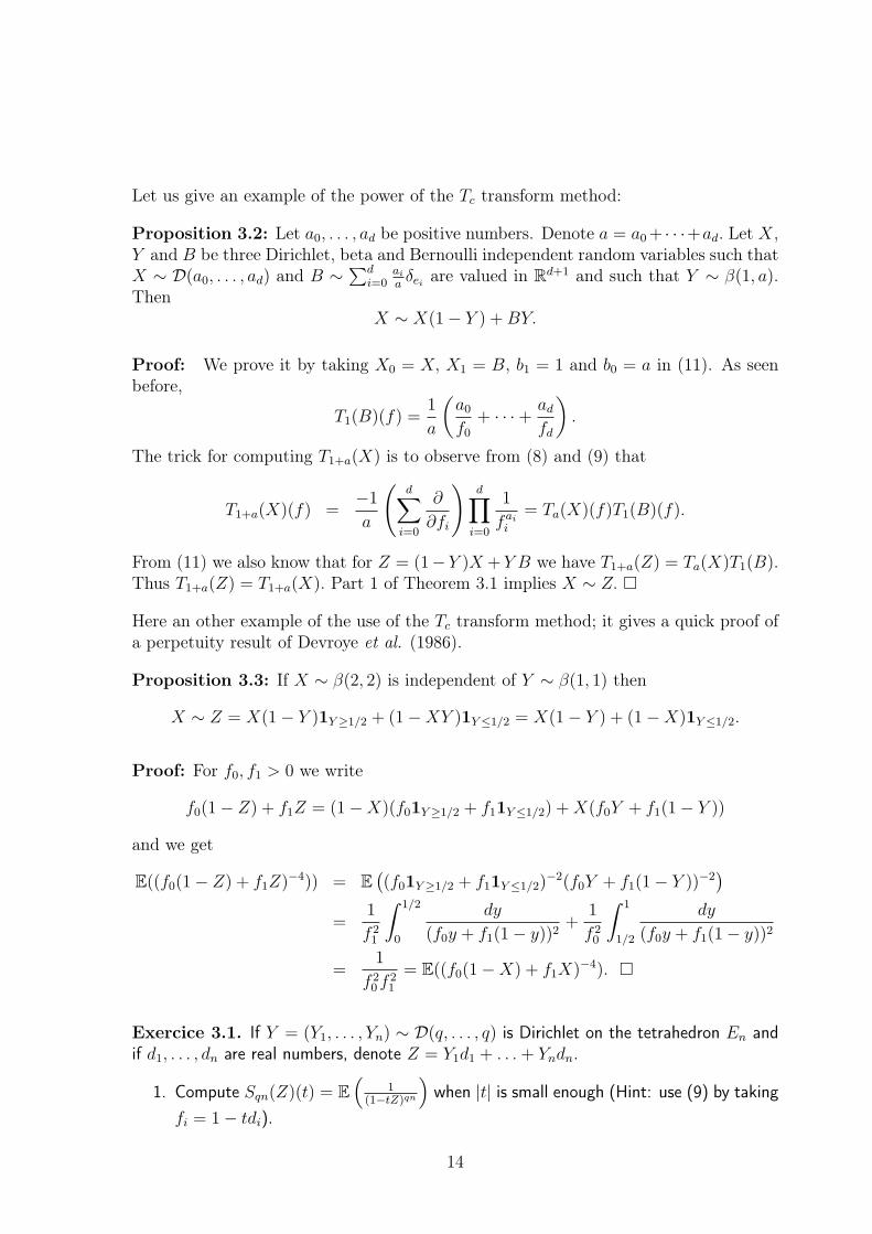
Let us give an example of the power of the Tc transform method:

Proposition 3.2: Let a0, . . . , ad be positive numbers. Denote a = a0+ · · ·+ad. Let X,Y and B be three Dirichlet, beta and Bernoulli independent random variables such thatX ∼ D(a0, . . . , ad) and B ∼∑d

i=0aiaδei are valued in R

d+1 and such that Y ∼ β(1, a).Then

X ∼ X(1− Y ) +BY.

Proof: We prove it by taking X0 = X, X1 = B, b1 = 1 and b0 = a in (11). As seenbefore,

T1(B)(f) =1

a

(

a0f0

+ · · ·+ adfd

)

.

The trick for computing T1+a(X) is to observe from (8) and (9) that

T1+a(X)(f) =−1

a

(

d∑

i=0

∂

∂fi

)

d∏

i=0

1

faii

= Ta(X)(f)T1(B)(f).

From (11) we also know that for Z = (1−Y )X +Y B we have T1+a(Z) = Ta(X)T1(B).Thus T1+a(Z) = T1+a(X). Part 1 of Theorem 3.1 implies X ∼ Z.

Here an other example of the use of the Tc transform method; it gives a quick proof ofa perpetuity result of Devroye et al. (1986).

Proposition 3.3: If X ∼ β(2, 2) is independent of Y ∼ β(1, 1) then

X ∼ Z = X(1− Y )1Y≥1/2 + (1−XY )1Y≤1/2 = X(1− Y ) + (1−X)1Y≤1/2.

Proof: For f0, f1 > 0 we write

f0(1− Z) + f1Z = (1−X)(f01Y≥1/2 + f11Y≤1/2) +X(f0Y + f1(1− Y ))

and we get

E((f0(1− Z) + f1Z)−4)) = E

(

(f01Y≥1/2 + f11Y≤1/2)−2(f0Y + f1(1− Y ))−2

)

=1

f 21

∫ 1/2

0

dy

(f0y + f1(1− y))2+

1

f 20

∫ 1

1/2

dy

(f0y + f1(1− y))2

=1

f 20 f

21

= E((f0(1−X) + f1X)−4).

Exercice 3.1. If Y = (Y1, . . . , Yn) ∼ D(q, . . . , q) is Dirichlet on the tetrahedron En andif d1, . . . , dn are real numbers, denote Z = Y1d1 + . . .+ Yndn.

1. Compute Sqn(Z)(t) = E

(

1(1−tZ)qn

)

when |t| is small enough (Hint: use (9) by taking

fi = 1− tdi).

14

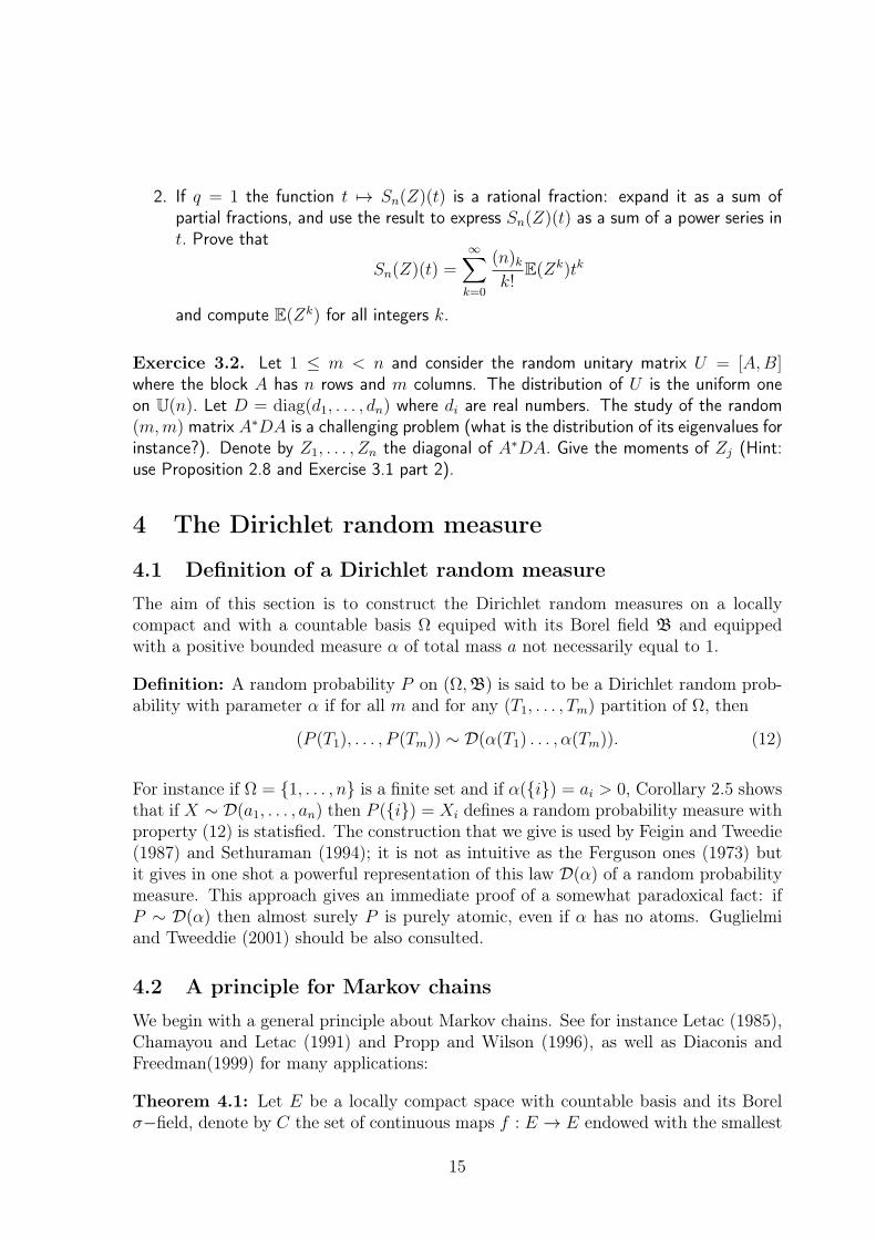
2. If q = 1 the function t 7→ Sn(Z)(t) is a rational fraction: expand it as a sum ofpartial fractions, and use the result to express Sn(Z)(t) as a sum of a power series int. Prove that

Sn(Z)(t) =∞∑

k=0

(n)kk!

E(Zk)tk

and compute E(Zk) for all integers k.

Exercice 3.2. Let 1 ≤ m < n and consider the random unitary matrix U = [A,B]where the block A has n rows and m columns. The distribution of U is the uniform oneon U(n). Let D = diag(d1, . . . , dn) where di are real numbers. The study of the random(m,m) matrix A∗DA is a challenging problem (what is the distribution of its eigenvalues forinstance?). Denote by Z1, . . . , Zn the diagonal of A∗DA. Give the moments of Zj (Hint:use Proposition 2.8 and Exercise 3.1 part 2).

4 The Dirichlet random measure

4.1 Definition of a Dirichlet random measure

The aim of this section is to construct the Dirichlet random measures on a locallycompact and with a countable basis Ω equiped with its Borel field B and equippedwith a positive bounded measure α of total mass a not necessarily equal to 1.

Definition: A random probability P on (Ω,B) is said to be a Dirichlet random prob-ability with parameter α if for all m and for any (T1, . . . , Tm) partition of Ω, then

(P (T1), . . . , P (Tm)) ∼ D(α(T1) . . . , α(Tm)). (12)

For instance if Ω = 1, . . . , n is a finite set and if α(i) = ai > 0, Corollary 2.5 showsthat if X ∼ D(a1, . . . , an) then P (i) = Xi defines a random probability measure withproperty (12) is statisfied. The construction that we give is used by Feigin and Tweedie(1987) and Sethuraman (1994); it is not as intuitive as the Ferguson ones (1973) butit gives in one shot a powerful representation of this law D(α) of a random probabilitymeasure. This approach gives an immediate proof of a somewhat paradoxical fact: ifP ∼ D(α) then almost surely P is purely atomic, even if α has no atoms. Guglielmiand Tweeddie (2001) should be also consulted.

4.2 A principle for Markov chains

We begin with a general principle about Markov chains. See for instance Letac (1985),Chamayou and Letac (1991) and Propp and Wilson (1996), as well as Diaconis andFreedman(1999) for many applications:

Theorem 4.1: Let E be a locally compact space with countable basis and its Borelσ−field, denote by C the set of continuous maps f : E → E endowed with the smallest

15

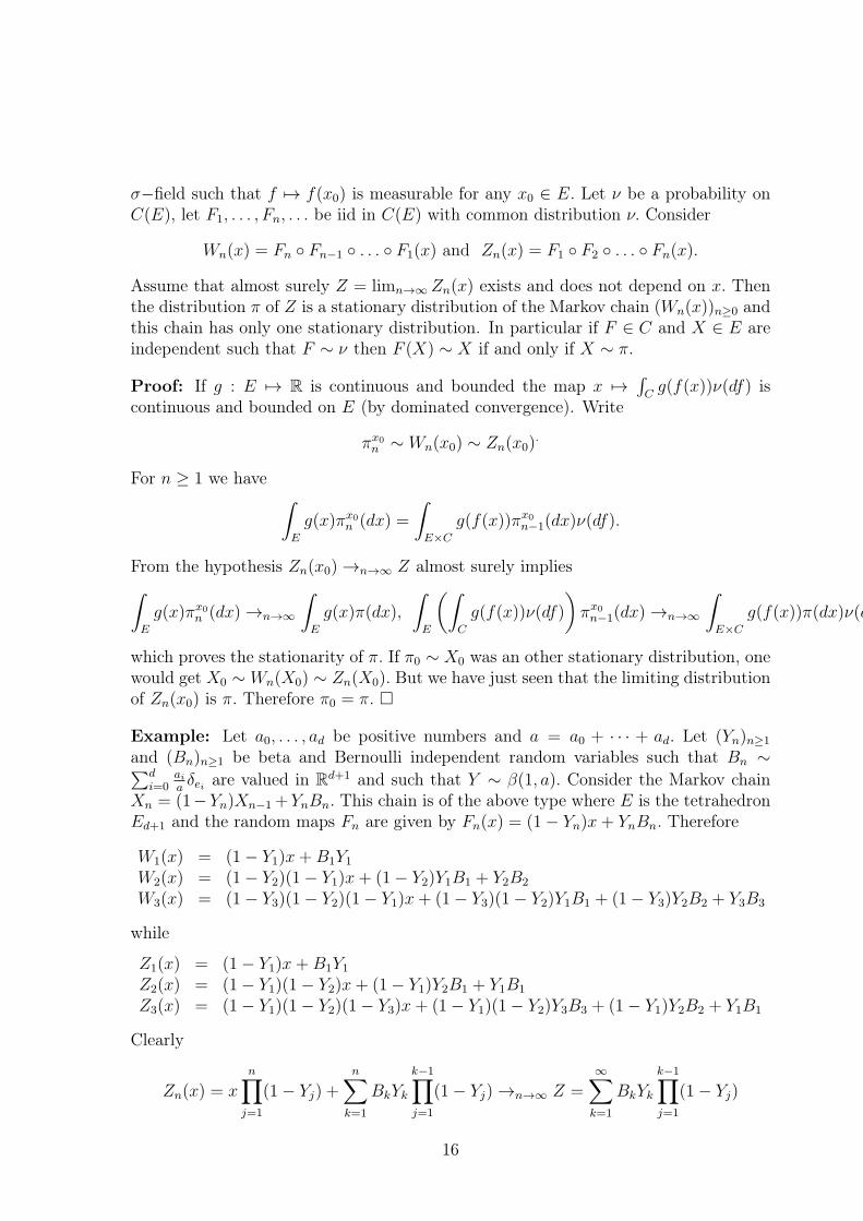
σ−field such that f 7→ f(x0) is measurable for any x0 ∈ E. Let ν be a probability onC(E), let F1, . . . , Fn, . . . be iid in C(E) with common distribution ν. Consider

Wn(x) = Fn Fn−1 . . . F1(x) and Zn(x) = F1 F2 . . . Fn(x).

Assume that almost surely Z = limn→∞ Zn(x) exists and does not depend on x. Thenthe distribution π of Z is a stationary distribution of the Markov chain (Wn(x))n≥0 andthis chain has only one stationary distribution. In particular if F ∈ C and X ∈ E areindependent such that F ∼ ν then F (X) ∼ X if and only if X ∼ π.

Proof: If g : E 7→ R is continuous and bounded the map x 7→∫

Cg(f(x))ν(df) is

continuous and bounded on E (by dominated convergence). Write

πx0

n ∼ Wn(x0) ∼ Zn(x0).

For n ≥ 1 we have∫

E

g(x)πx0

n (dx) =

∫

E×C

g(f(x))πx0

n−1(dx)ν(df).

From the hypothesis Zn(x0) →n→∞ Z almost surely implies

∫

E

g(x)πx0

n (dx) →n→∞

∫

E

g(x)π(dx),

∫

E

(∫

C

g(f(x))ν(df)

)

πx0

n−1(dx) →n→∞

∫

E×C

g(f(x))π(dx)ν(d

which proves the stationarity of π. If π0 ∼ X0 was an other stationary distribution, onewould get X0 ∼ Wn(X0) ∼ Zn(X0). But we have just seen that the limiting distributionof Zn(x0) is π. Therefore π0 = π.

Example: Let a0, . . . , ad be positive numbers and a = a0 + · · · + ad. Let (Yn)n≥1

and (Bn)n≥1 be beta and Bernoulli independent random variables such that Bn ∼∑d

i=0aiaδei are valued in R

d+1 and such that Y ∼ β(1, a). Consider the Markov chainXn = (1−Yn)Xn−1+YnBn. This chain is of the above type where E is the tetrahedronEd+1 and the random maps Fn are given by Fn(x) = (1− Yn)x+ YnBn. Therefore

W1(x) = (1− Y1)x+ B1Y1

W2(x) = (1− Y2)(1− Y1)x+ (1− Y2)Y1B1 + Y2B2

W3(x) = (1− Y3)(1− Y2)(1− Y1)x+ (1− Y3)(1− Y2)Y1B1 + (1− Y3)Y2B2 + Y3B3

while

Z1(x) = (1− Y1)x+ B1Y1

Z2(x) = (1− Y1)(1− Y2)x+ (1− Y1)Y2B1 + Y1B1

Z3(x) = (1− Y1)(1− Y2)(1− Y3)x+ (1− Y1)(1− Y2)Y3B3 + (1− Y1)Y2B2 + Y1B1

Clearly

Zn(x) = xn∏

j=1

(1− Yj) +n∑

k=1

BkYk

k−1∏

j=1

(1− Yj) →n→∞ Z =∞∑

k=1

BkYk

k−1∏

j=1

(1− Yj)

16

From Proposition 3.2 we can claim that π = D(a0, . . . , ad) is a stationary distributionof this Markow chain, from Theorem 4.1 we can claim that Z ∼ π or

∞∑

k=1

BkYk

k−1∏

j=1

(1− Yj) ∼ D(a0, . . . , ad), (13)

an important result for the next section.

Exercice 4.2.1 If X and Y are independent such that X ∼ βp,p+q and Y ∼ βp,q showthat X ∼ Y (1−X) (Hint: compute the Mellin transform of X, 1−X and Y with the helpof Section 1). If (Yk)k≥1 are iid such that Yk ∼ βp,q consider the Markov chain (Xn)n≥0

on (0, 1) defined by Xn = Yn(1−Xn−1). By applying Theorem 4.2 to Fn(x) = Yn(1− x),compute Wn(x) and Zn(x). Show that Z = limZn(x) exists, express it in terms of the(Yk)k≥1’s and give its distribution π (source, Chamayou and Letac (1991) pages 19-20)

Exercice 4.2.2 If X and Y are independent such that X ∼ β(2)p,q and Y ∼ β

(2)p,p+q show

that X ∼ Y (1+X) (Hint: compute the Mellin transform of X, 1+X and Y with the help

of Section 1). If (Yk)k≥1 are iid such that Yk ∼ β(2)p,p+q consider the Markov chain (Xn)n≥0

on (0, 1) defined by Xn = Yn(1 +Xn−1). By applying Theorem 4.2 to Fn(x) = Yn(1 + x),compute Wn(x) and Zn(x). Show that Z = limZn(x) exists, express it in terms of the(Yk)k≥1’s and give its distribution π (source, Chamayou and Letac (1991) page 21)

Exercice 4.2.3 If X and Y are independent such that X ∼ β1/3,2/3 and Y ∼ β1/2,1/3

show that X ∼ Y (1−X)2 (Hint: compute the Mellin transform of X, 1−X and Y withthe help of Section 1). If (Yk)k≥1 are iid such that Yk ∼ β1/2,1/3 consider the Markov chain(Xn)n≥0 on (0, 1) defined by Xn = Yn(1 −Xn−1)

2. Admitting that Z = limZn(x) exists,give its distribution π (source, Chamayou and Letac (1991) page 27-29, where the existenceof Z is proved)

4.3 Construction of the Dirichlet random measure

Theorem 4.2: Let Ω be locally compact with countable topological basis equipedwith its Borel σ field, and let α be a positive bounded measure on Ω of total massa. Let X1, Y1, . . . , Xn, Yn, . . . be independent random variables such that yj ∼ β1,a andsuch that Xj is valued in Ω with distribution α/a. Then the distribution of the randomprobability

P =∞∑

k=1

δXkYk

k−1∏

j=1

(1− Yj) (14)

is Dirichlet with parameter α.

Proof: We fix a partition (T1, . . . , Tm) of Ω and we define Bk = (1, 0, . . . , 0) = e1 ifXk ∈ T1, Bk = (0, 1, . . . , 0) = e2 if Xk ∈ T2,..., Bk = (0, 0, . . . , 1) = em if Xk ∈ Tm.Here e1, . . . , em is the canonical basis of Rm. Therefore Bk is Bernoulli distributed in

17

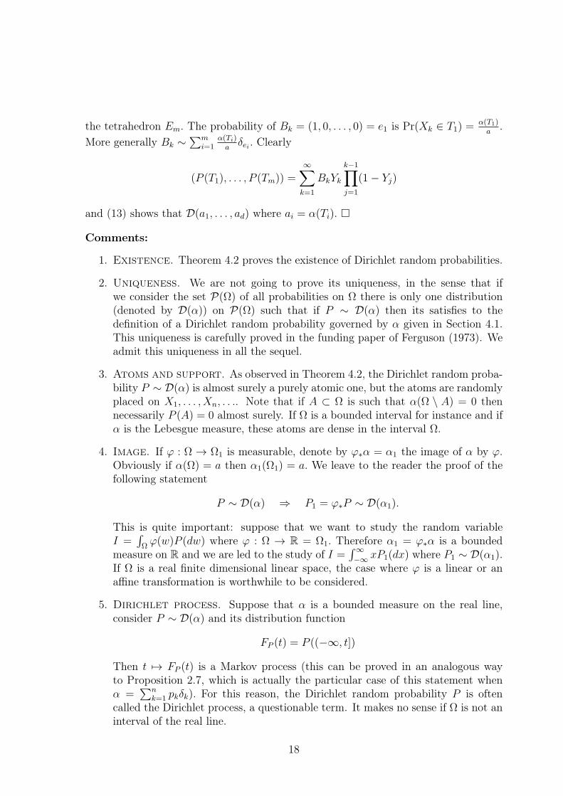
the tetrahedron Em. The probability of Bk = (1, 0, . . . , 0) = e1 is Pr(Xk ∈ T1) =α(T1)

a.

More generally Bk ∼∑m

i=1α(Ti)a

δei . Clearly

(P (T1), . . . , P (Tm)) =∞∑

k=1

BkYk

k−1∏

j=1

(1− Yj)

and (13) shows that D(a1, . . . , ad) where ai = α(Ti).

Comments:

1. Existence. Theorem 4.2 proves the existence of Dirichlet random probabilities.

2. Uniqueness. We are not going to prove its uniqueness, in the sense that ifwe consider the set P(Ω) of all probabilities on Ω there is only one distribution(denoted by D(α)) on P(Ω) such that if P ∼ D(α) then its satisfies to thedefinition of a Dirichlet random probability governed by α given in Section 4.1.This uniqueness is carefully proved in the funding paper of Ferguson (1973). Weadmit this uniqueness in all the sequel.

3. Atoms and support. As observed in Theorem 4.2, the Dirichlet random proba-bility P ∼ D(α) is almost surely a purely atomic one, but the atoms are randomlyplaced on X1, . . . , Xn, . . .. Note that if A ⊂ Ω is such that α(Ω \ A) = 0 thennecessarily P (A) = 0 almost surely. If Ω is a bounded interval for instance and ifα is the Lebesgue measure, these atoms are dense in the interval Ω.

4. Image. If ϕ : Ω → Ω1 is measurable, denote by ϕ∗α = α1 the image of α by ϕ.Obviously if α(Ω) = a then α1(Ω1) = a. We leave to the reader the proof of thefollowing statement

P ∼ D(α) ⇒ P1 = ϕ∗P ∼ D(α1).

This is quite important: suppose that we want to study the random variableI =

∫

Ωϕ(w)P (dw) where ϕ : Ω → R = Ω1. Therefore α1 = ϕ∗α is a bounded

measure on R and we are led to the study of I =∫∞

−∞xP1(dx) where P1 ∼ D(α1).

If Ω is a real finite dimensional linear space, the case where ϕ is a linear or anaffine transformation is worthwhile to be considered.

5. Dirichlet process. Suppose that α is a bounded measure on the real line,consider P ∼ D(α) and its distribution function

FP (t) = P ((−∞, t])

Then t 7→ FP (t) is a Markov process (this can be proved in an analogous wayto Proposition 2.7, which is actually the particular case of this statement whenα =

∑nk=1 pkδk). For this reason, the Dirichlet random probability P is often

called the Dirichlet process, a questionable term. It makes no sense if Ω is not aninterval of the real line.

18

Exercice 4.3.1. (Yamato, 1984) If Y1, . . . , Yk, . . . are iid with Yk ∼ β1,a, denote

Pk = Yk

k−1∏

j=1

(1− Yj)

(see (14)). Compute E(Y 2k ), E((1− Yk)

2), E(P 2k ) and E(

∑∞k=1 P

2k ).

5 The random variable∫

Ω g(w)P (dw) when P ∼ D(α).

Given a random Dirichlet measure on Ω governed by α and given a real function g on Ωour next task is to study Ig =

∫

Ωg(w)P (dw). If the image of α by g is α1 on the real line

and if P1 ∼ D(α1) this integral becomes Ig =∫∞

−∞xP1(dx). We first solve the existence

problem, and we next consider the difficult question: what is the distribution of Ig interms of α? In this section we deal with general facts and we are more specific whenthe mass a of α is one. In this case, a powerful tool is the ordinary Cauchy Stieltjestransform of a bounded measure on the real line. Section 6 will deal with general a.

5.1 Existence of∫

Ω g(w)P (dw)

We begin with an obvious generalization of (9):

Theorem 5.1. Let α be a bounded measure on Ω of total mass a, and let P ∼ D(α).If f : Ω → (0,∞) is such that there exists 0 < m with m ≤ f(w) ≤ M for all w ∈ Ωand if I − f =

∫

Ωg(w)P (dw) then

E

(

1

(If )a

)

= e−∫Ωlog f(w)α(dw) (15)

Proof. If f takes only a finite number of values, (15) is nothing but (9). In the generalcase there exists an increasing sequence fn taking each a finite number of values suchthat lim fn(w) = f(w) for all w. Therefore Ifn →n→∞ If and

∫

Ωlog fn(w)α(dw) →n→∞

∫

Ωlog f(w)α(dw) by monotone convergence. Also Ifn increases towards If , therefore

I−afn

decreases towards I−af . Since E

(

1(If )a

)

≤ 1ma is finite, the theorem of monotone

decreasing convergence can be applied to claim that the limit of E(

1(Ifn )

a

)

is E(

1(If )a

)

and this ends the proof. .

If α is a bounded measure of total mass a on Ω = Rd with bounded support formula

(15) may be quite sufficient for finding the distribution µα of X =∫

Rd xP (dx) whenP ∼ D(α). If we apply (15) to f(x) = 1 + t〈y, x〉 where t is small enough such that1 + t〈y, x〉 is positive on the support of α, we get a way to find the moments of 〈y,X〉by expanding both sides of

∫

Rd

µα(dx)

(1 + t〈y, x〉)a = e−∫Rd

log(1+t〈y,w〉)α(dw)

19

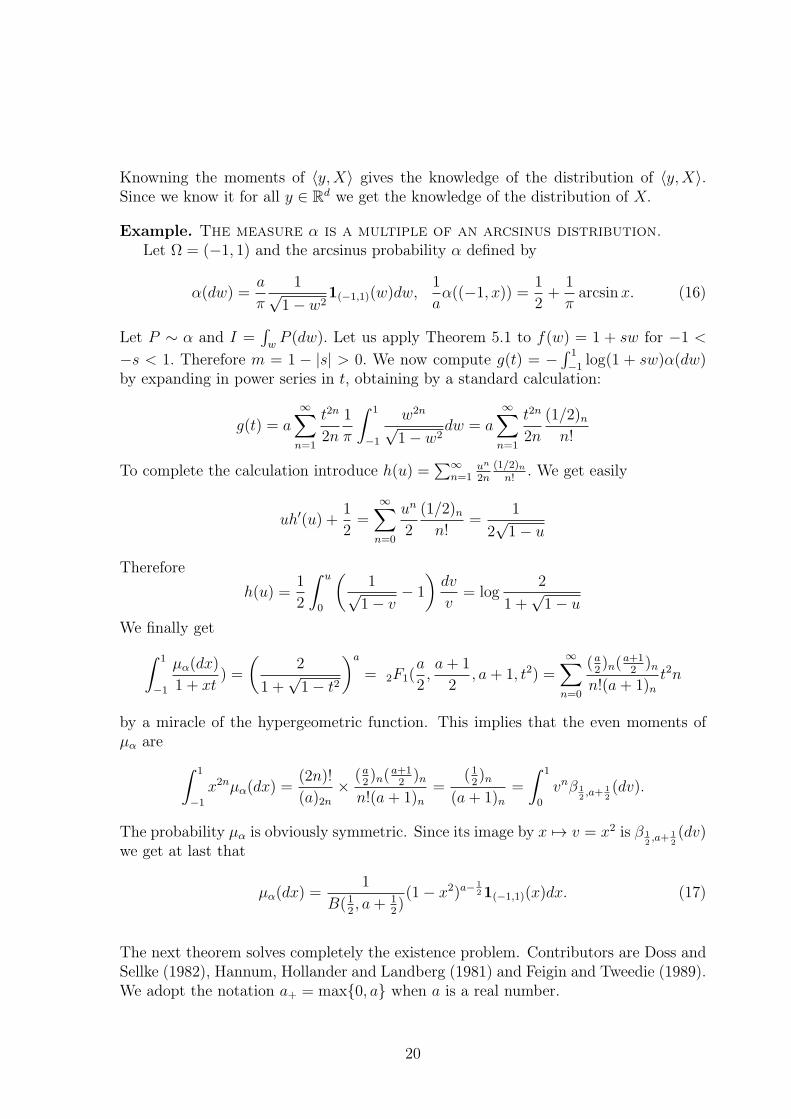
Knowning the moments of 〈y,X〉 gives the knowledge of the distribution of 〈y,X〉.Since we know it for all y ∈ R

d we get the knowledge of the distribution of X.

Example. The measure α is a multiple of an arcsinus distribution.Let Ω = (−1, 1) and the arcsinus probability α defined by

α(dw) =a

π

1√1− w2

1(−1,1)(w)dw,1

aα((−1, x)) =

1

2+

1

πarcsin x. (16)

Let P ∼ α and I =∫

wP (dw). Let us apply Theorem 5.1 to f(w) = 1 + sw for −1 <

−s < 1. Therefore m = 1 − |s| > 0. We now compute g(t) = −∫ 1

−1log(1 + sw)α(dw)

by expanding in power series in t, obtaining by a standard calculation:

g(t) = a∞∑

n=1

t2n

2n

1

π

∫ 1

−1

w2n

√1− w2

dw = a∞∑

n=1

t2n

2n

(1/2)nn!

To complete the calculation introduce h(u) =∑∞

n=1un

2n(1/2)n

n!. We get easily

uh′(u) +1

2=

∞∑

n=0

un

2

(1/2)nn!

=1

2√1− u

Therefore

h(u) =1

2

∫ u

0

(

1√1− v

− 1

)

dv

v= log

2

1 +√1− u

We finally get

∫ 1

−1

µα(dx)

1 + xt) =

(

2

1 +√1− t2

)a

= 2F1(a

2,a+ 1

2, a+ 1, t2) =

∞∑

n=0

(a2)n(

a+12)n

n!(a+ 1)nt2n

by a miracle of the hypergeometric function. This implies that the even moments ofµα are

∫ 1

−1

x2nµα(dx) =(2n)!

(a)2n× (a

2)n(

a+12)n

n!(a+ 1)n=

(12)n

(a+ 1)n=

∫ 1

0

vnβ 1

2,a+ 1

2(dv).

The probability µα is obviously symmetric. Since its image by x 7→ v = x2 is β 1

2,a+ 1

2(dv)

we get at last that

µα(dx) =1

B(12, a+ 1

2)(1− x2)a−

1

21(−1,1)(x)dx. (17)

The next theorem solves completely the existence problem. Contributors are Doss andSellke (1982), Hannum, Hollander and Landberg (1981) and Feigin and Tweedie (1989).We adopt the notation a+ = max0, a when a is a real number.

20

Theorem 5.2: Let Ω be a complete metric space, α be a positive bounded measureon Ω of total mass 1 and let P ∼ D(α). If g is a positive measurable function on Ωthen

∫

Ωg(w)P (dw) < ∞ almost surely if and only if

∫

Ω(log g(w))+α(dw) < ∞

Proof: We show first Part ⇐ . We write f(w) = (log g(w))+. By definition

∫

Ω

g(w)P (dw) ≤∫

Ω

max(1, g(w))P (dw) = limn→∞

n∑

k=1

ef(Xk)Yk

k−1∏

j=1

(1− Yj) ≤ ∞.

Since 1−Yk ∼ β(a, 1) then E(log(1−Yk)) = a∫ 1

0ya−1 log y dy = − 1

aand the law of the

large numbers implies that almost surely

limk→∞

(

k−1∏

j=1

(1− Yj)

)1/k

= e−1/a.

The fact that E(f(X1)) < ∞ implies that E(f(X1)) =∫∞

0Pr(f(X1) ≥ x)dx < ∞. As a

consequence for each ε > 0 we have∑∞

n=1 Pr(f(X1) ≥ nε) < ∞), a fact that we preferto write as follows

∞∑

n=1

Pr(f(Xn)

n≥ ε) < ∞).

From the Borel Cantelli Lemma, this implies that the set of integers n; f(Xn)n

≥ ε is

almost surely finite, or that lim supn→∞f(Xn)

n≤ ε almost surely. Since this true for all

ε we have limn→∞f(Xn)

n= 0 since f ≥ 0. In the same manner we have limk→∞

log Yk

k= 0

and limk→∞ Y1/kk = 0. We now use the Cauchy criteria of convergence of a series with

positive terms uk saying that if lim supk→∞k√uk = r < 1 then

∑∞k=1 uk converges. We

apply it to

uk = ef(Xk)Yk

k−1∏

j=1

(1− Yj).

The above considerations have shown that limk→∞k√uk ≤ e−

1

a = r < 1. This provesPart ⇐ .

We now show Part ⇒ . We suppose that∫

Ω(log g(w))+α(dw) = ∞ and we want to

show that for all real x we have

Pr(

∫

Ω

g(w)P (dw) ≤ x) = 0.

A trick invented by Hannum et al (1981) is the following. Consider a bounded functionh and Ih =

∫

Ωh(w)P (dw), which exists, since h is bounded. Then from Theorem 5.1

applied to f(w) = 1 + sg(w) we have

E

(

1

(1 + sIh)a

)

= e−∫Ωlog(1+s h(w))α(dw). (18)

21

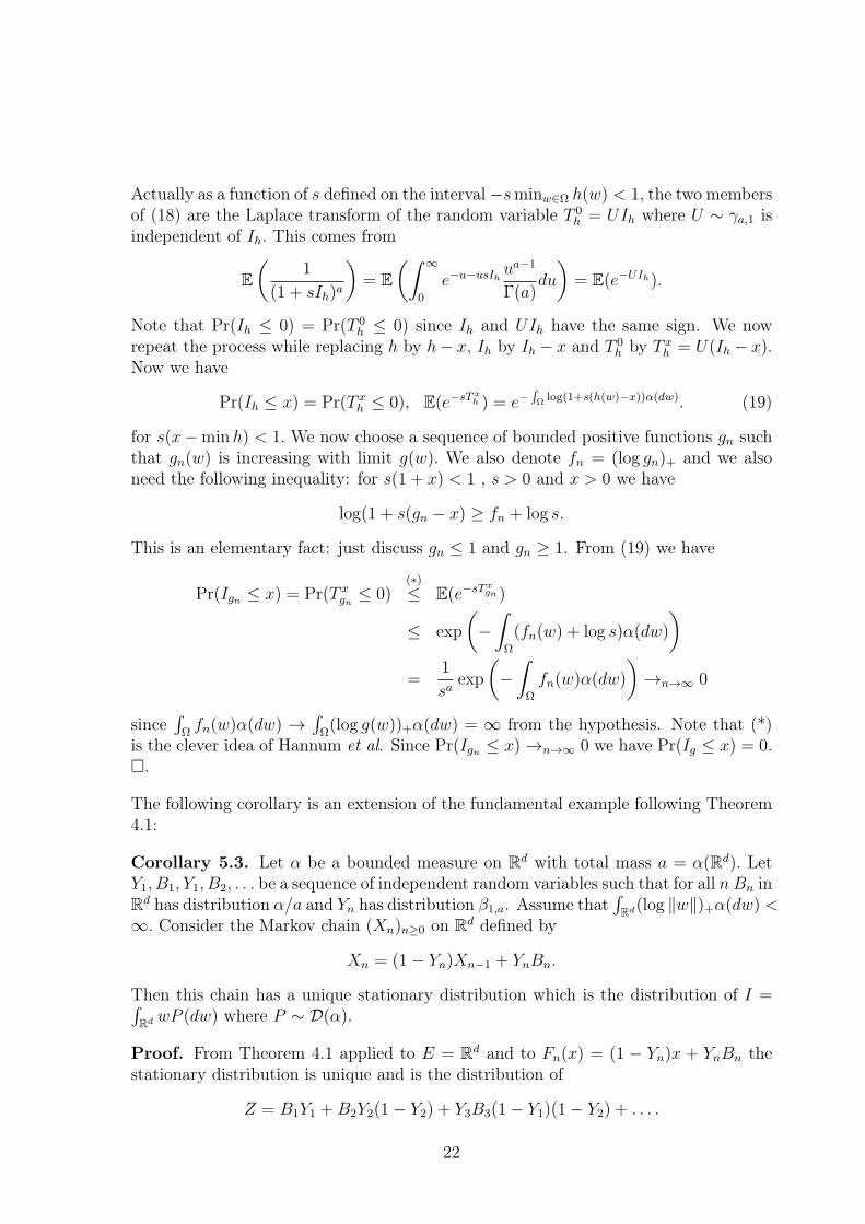
Actually as a function of s defined on the interval −sminw∈Ω h(w) < 1, the two membersof (18) are the Laplace transform of the random variable T 0

h = UIh where U ∼ γa,1 isindependent of Ih. This comes from

E

(

1

(1 + sIh)a

)

= E

(∫ ∞

0

e−u−usIhua−1

Γ(a)du

)

= E(e−UIh).

Note that Pr(Ih ≤ 0) = Pr(T 0h ≤ 0) since Ih and UIh have the same sign. We now

repeat the process while replacing h by h− x, Ih by Ih − x and T 0h by T x

h = U(Ih − x).Now we have

Pr(Ih ≤ x) = Pr(T xh ≤ 0), E(e−sTx

h ) = e−∫Ωlog(1+s(h(w)−x))α(dw). (19)

for s(x−minh) < 1. We now choose a sequence of bounded positive functions gn suchthat gn(w) is increasing with limit g(w). We also denote fn = (log gn)+ and we alsoneed the following inequality: for s(1 + x) < 1 , s > 0 and x > 0 we have

log(1 + s(gn − x) ≥ fn + log s.

This is an elementary fact: just discuss gn ≤ 1 and gn ≥ 1. From (19) we have

Pr(Ign ≤ x) = Pr(T xgn ≤ 0)

(∗)

≤ E(e−sTxgn )

≤ exp

(

−∫

Ω

(fn(w) + log s)α(dw)

)

=1

saexp

(

−∫

Ω

fn(w)α(dw)

)

→n→∞ 0

since∫

Ωfn(w)α(dw) →

∫

Ω(log g(w))+α(dw) = ∞ from the hypothesis. Note that (*)

is the clever idea of Hannum et al. Since Pr(Ign ≤ x) →n→∞ 0 we have Pr(Ig ≤ x) = 0..

The following corollary is an extension of the fundamental example following Theorem4.1:

Corollary 5.3. Let α be a bounded measure on Rd with total mass a = α(Rd). Let

Y1, B1, Y1, B2, . . . be a sequence of independent random variables such that for all n Bn inR

d has distribution α/a and Yn has distribution β1,a. Assume that∫

Rd(log ‖w‖)+α(dw) <∞. Consider the Markov chain (Xn)n≥0 on R

d defined by

Xn = (1− Yn)Xn−1 + YnBn.

Then this chain has a unique stationary distribution which is the distribution of I =∫

Rd wP (dw) where P ∼ D(α).

Proof. From Theorem 4.1 applied to E = Rd and to Fn(x) = (1 − Yn)x + YnBn the

stationary distribution is unique and is the distribution of

Z = B1Y1 + B2Y2(1− Y2) + Y3B3(1− Y1)(1− Y2) + . . . .

22

From Theorem 5.2 since∫

Rd(log ‖w‖)+α(dw) < ∞ the random integral I =∫

Rd wP (dw)converges absolutely when P ∼ D(α). Furthermore Theorem 4.2 from (14) says thatthe random probability P has the distribution of

Q =∞∑

k=1

δBkYk

k−1∏

j=1

(1− Yj).

Hence

I =

∫

Rd

wP (dw) ∼ Z =

∫

Rd

wQ(dw) =∞∑

k=1

BkYk

k−1∏

j=1

(1− Yj).

Exercice 5.1.1. (Cauchy distribution ,Yamato 1984) If z = p + iq is a complexnumber with q > 0 define the Cauchy distribution on the real line

cz(dx) =1

π

qdx

(x− p)2 + q2

Show that if t > 0∫ ∞

−∞

eixtcz(t) = eizt

(Hint, prove that if X ∼ ci then E(eiXt) = e−|t| and that qX + p ∼ cz). What is thevalue of this integral if t < 0? Consider now the random Dirichlet distribution P ∼ D(acz).Using Theorem 5.2 show that I =

∫∞

−∞xP (dx) converges almost surely. Express I using

(14). Using the fact that∑∞

k=1 Pk = 1 when Pk = Yk

∏k−1j=1(1− Yj), prove that I ∼ cz for

all a (Hint, consider its characteristic function E(eitI)).

Exercice 5.1.2. If α is a bounded measure on R such that∫∞

−∞(log |x|)+α(dx) < ∞, let

P ∼ D(α). Explain why the moments of∫∞

−∞xnP (dx) always exist. Give an example of

an α such that P has moments but no exponential moments .

5.2 Tutorial on the Cauchy Stieltjes transform

Among the various extensions of Theorem 5.1 the one considered in Theorem 5.9 belowis particularly attractive. To introduce it we use some mathematical results describedin this section. We consider the analytic function z 7→ log z defined on the complexplane without the negative part of the real axis by log z = log |z| + iθ when z = |z|eiθwith θ ∈ (−π, π). The derivative of this analytic function is 1/z. Furthermore, theexponential of a log z is denoted by za. With these conventions, if µ is a probability onthe real line, we define the Cauchy-Stieltjes transform of µ of type c > 0 as the functionof z defined on the upper complex half plane =z > 0 by

z 7→∫ ∞

−∞

µ(dw)

(w − z)c.

23

This integral converges since∣

∣

∣

∣

1

(w − z)c

∣

∣

∣

∣

≤ 1

|=z|c .

It is sometimes called the generalized Cauchy-Stieltjes transform. If c = 1 one talkssimply about the Cauchy-Stieltjes transform of µ. This section gives information mainlyabout about the case c = 1.

Theorem 5.4. Let H+ = z;=z > 0 be the upper half complex plane. Let µ be aprobability on R and consider the map on H+

z 7→ sµ(z) =

∫ ∞

−∞

µ(dw)

w − z

called the Cauchy Stieltjes transform of µ. Then sµ(z) exists and is valued in H+ andµ 7→ sµ characterizes µ : more specifically if (a, b) are not atoms of µ we have

limy↓0

1

π

∫ b

a

=sµ(x+ iy)dx = µ([a, b]). (20)

Finally if X ∼ µ and aX + b ∼ µ1 with a > 0 then sµ1(z) = 1

asµ(

z−ba).

Proof. Clearly

<sµ(x+ iy) =

∫ ∞

−∞

(w − x)µ(dw)

(w − x)2 + y2, =sµ(x+ iy) = y

∫ ∞

−∞

µ(dw)

(w − x)2 + y2

and this proves the existence and the fact that sµ(x + iy) ∈ H+ for y > 0. Now recallthat for y > 0 the characteristic function of the Cauchy distribution

cz(dw) = cx+iy(dw) =1

π

ydw

(w − x)2 + y2

is

ϕcx+iy(t) =

∫ ∞

−∞

eitxwcx+iy(dw) = e−y|t|+ixt

or is eitz for t > 0. This implies that for fixed y > 0 then x 7→ 1π=sµ(x + iy) is the

density of a probability µy with characteristic function

ϕµy(t) = e−y|t|ϕµ(t).

Clearly µ is determined from µy. One observes that limy→0 µy = µ for tight convergence.With the Paul Lévy theorem we get (20). The last formula is obvious.

Corollary 5.5. Cauchy Stieltjes transform of type c if c is an integer.If µ is a probability on R whith Cauchy Stieltjes transform sµ and if c is a positiveinteger, then the Cauchy Stieltjes transform of type c of µ is

∫ ∞

−∞

µ(dw)

(w − z)c= (c− 1)!s(c)µ (z)

24

and it characterizes µ.

Proof. The only thing to prove is that it characterizes µ. We show it by inductionon c. For c = 1 this has been proved by Theorem 5.1. If true for c, suppose that weknow f(z) = 1

c!

∫∞

−∞µ(dw)

(w−z)c+1 . Then s(c)µ (z) is the only primitive of f which vanishes

when |z| → ∞ along the imaginary axis, and this shows that f characterizes s(c)µ . The

induction follows.

Remark. If c > 0 is not an integer, the fact that the Cauchy Stieltjes of µ of type c,namely the function z 7→ f(z) =

∫∞

−∞µ(dw)(w−z)c

on the upper half plane H+ characterizesµ is harder to prove and we will do it only in Section 6.

The next three propositions of this section will give useful examples of CauchyStieltjes transforms.

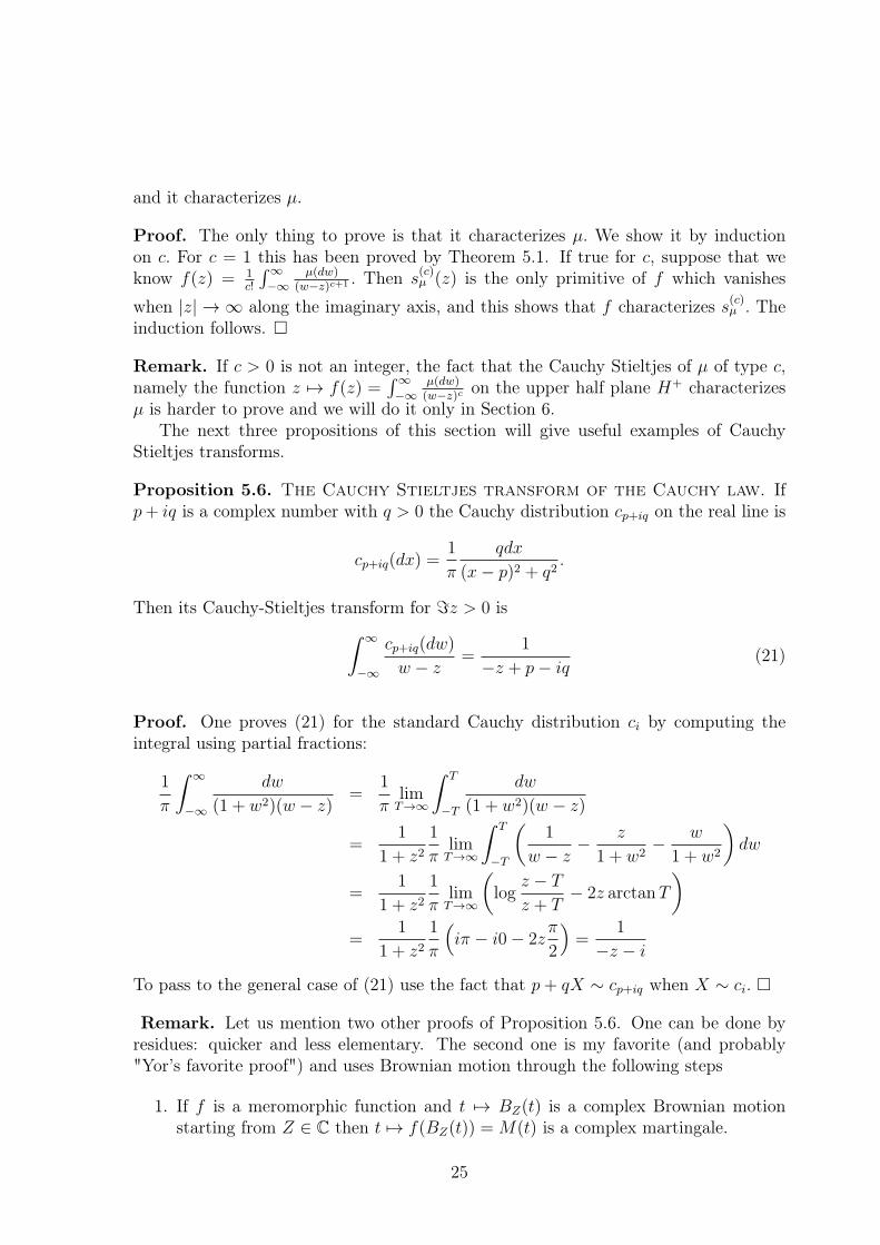
Proposition 5.6. The Cauchy Stieltjes transform of the Cauchy law. Ifp+ iq is a complex number with q > 0 the Cauchy distribution cp+iq on the real line is

cp+iq(dx) =1

π

qdx

(x− p)2 + q2.

Then its Cauchy-Stieltjes transform for =z > 0 is

∫ ∞

−∞

cp+iq(dw)

w − z=

1

−z + p− iq(21)

Proof. One proves (21) for the standard Cauchy distribution ci by computing theintegral using partial fractions:

1

π

∫ ∞

−∞

dw

(1 + w2)(w − z)=

1

πlimT→∞

∫ T

−T

dw

(1 + w2)(w − z)

=1

1 + z21

πlimT→∞

∫ T

−T

(

1

w − z− z

1 + w2− w

1 + w2

)

dw

=1

1 + z21

πlimT→∞

(

logz − T

z + T− 2z arctanT

)

=1

1 + z21

π

(

iπ − i0− 2zπ

2

)

=1

−z − i

To pass to the general case of (21) use the fact that p+ qX ∼ cp+iq when X ∼ ci.

Remark. Let us mention two other proofs of Proposition 5.6. One can be done byresidues: quicker and less elementary. The second one is my favorite (and probably"Yor’s favorite proof") and uses Brownian motion through the following steps

1. If f is a meromorphic function and t 7→ BZ(t) is a complex Brownian motionstarting from Z ∈ C then t 7→ f(BZ(t)) = M(t) is a complex martingale.

25

2. If T is a regular stopping time, f(Z) = E(f(BZ(T )).

3. If Z ∈ H+ and if T is the hitting time of R then taking f(Z) = eitZ with t > 0shows that the Fourier transform of the distribution of BZ(T ) is eitZ , thus thisdistribution is the Cauchy distribution cZ .

4. If z ∈ H+ then Z 7→ f(Z) = 1Z−z

is analytic on H− = −H+. Let T be the hittingtime of R by BZ . We have

E

(

1

BZ(T )− z

)

=1

Z − z.

Since by symmetry the distribution of BZ(T ) is cZ we get the desired CauchyStieltjes transform of cZ .

Let us compute some other Cauchy Stieltjes transforms: The next proposition uses thehypergeometric function

F (a, b; c; z) =∞∑

n=0

zn

n!

(a)n(b)n(c)n

with the notation (a)0 = 1 and (a)n+1 = (a+ n)(a)n.

Proposition 5.7. The Cauchy Stieltjes transform of the beta law. TheCauchy Stieltjes transform of the distribution

βb,c−b(dw) =1

B(b, c− b)wb−1(1− w)c−b−1

1(0,1)(w)dw

is

sβb,c−b(z) = −1

zF (1, b, c; 1/z).

In particular

sβ3/2,3/2(z) = 2[1− 2z + 2

√

z(z − 1)] = −2[√z −

√z − 1]2.

If X ∼ β3/2,3/2 and Y = r(2X − 1) then the Stieltjes transform of the "Wigner halfcircle law" Wr of radius r is

sY (z) =1

r2[√z2 − r2 − z] = −2[

√z + r −

√z − r]2.

For r = σ√2 then s = sY satisfies

s2(z) +z

σ2s(z) +

1

σ2= 0. (22)

26

Proof. We use the Gauss formula∫ 1

0

wb−1(1− w)c−b−1(1− wz)−adt = B(b, c− b)F (a, b; c; z).

For getting the explicit result on sβ3/2,3/2we write

F (1, 3/2; 3; z) =∞∑

n=0

zn

(n+ 2)!(3/2)n

=1

z2

∞∑

n=0

zn+2

(n+ 2)!(3/2)n

=1

z2[−4(1− z)1/2 − 2z + 4]

= 2

(

1− (1− z)1/2

z

)2

(23)

The last example will not be used in this course, but is worthwhile to be known for itsrole in random matrix theory:

Proposition 5.8. The Cauchy Stieltjes transform of the Marchenko Pas-tur law. Let 0 < a < b. Then the following measure

A(dw) = Aa,b(dw) =4

π

1

(√b−√

a)21

w

√

(b− w)(w − a)1(a,b(w)dw

is a probability. Its Cauchy Stieltjes transform is

sA(z) =2

(√b−√

a)2z[√

(z − a)(z − b)− z +√ab].

and satisfies

z

(√b−√

a

2

)2

s2A(z) + (z −√ab)sA(z) + 1 = 0.

Proof. We compute first the integral

K(z) =

∫ b

a

1

w − z

√

(b− w)(w − a)dw.

The change of variable w = a+ (b− a)u gives

K(z) =(b− a)2

a− z

∫ 1

0

√

u(1− u)

1− a−ba−z

udu =

(b− a)2

a− zB(3/2, 3/2)F (1, 3/2; 3;

a− b

a− z)

from the Gauss formula. We use (23) and B(3/2, 3/2) = π/8 and we get

K(z) = −π

4[√z − b−

√z − a]2.

27

By considering K(0) we see easily that MP is a probability distribution. Now consider

I =

∫ b

a

1

w(w − z)

√

(b− w)(w − a)dw =1

z(K(z)−K(0))

Since sMP = I/K(0) we get the result.

Remark. For γ > 0 we now define the Marcenko Pastur law MPγ from Aa,b as follows:we take a(γ) = γ − 2

√γ + 1 and b(γ) = γ + 2

√γ + 1. We define MPγ(dw) as

For 0 < γ < 1 MPγ = (1− γ)δ0 + γAa(γ),b(γ)

For 1 ≤ γ MPγ = Aa(γ),b(γ).

For A = Aa(γ),b(γ) we can write

For γ ≥ 1 we have zs2A(z) + (z − γ + 1)sA(z) + 1 = 0.

For γ ≤ 1 we have zγs2A(z) + (z − 1 + γ)sA(z) + 1 = 0

Since for 0 < γ < 1 we have sMPγ (z) = −1−γz

+ γsA(z), this implies that for all y > 0the Cauchy Stieltjes transform of MPγ satisfies the important formula

zs2MPγ(z) + (z + 1− γ)sMPγ (z) + 1 = 0. (24)

Exercise 5.2.1. Let 0 < a < b and 0 < β < q + 1 where q is a non negative integer.Consider the following probability

A(dw) = C1

w(b− w)β−1(w − a)q−β

1(a,b)(w)dw.

Show that its Cauchy Stieltjes transform is sA(z) =F (z)F (0)

− 1 where

F (z) = (a− z)β−1(b− z)q−β −q−1∑

k=0

(β − q)kk!

(a− b)k(a− z)q−k−1.

Hint: compute first the integral

K(z) =

∫ b

a

1

w − z(b− w)β−1(w − a)q−βdw

=π

q! sin βπ

[

(a− z)β−1(b− z)q−β −q−1∑

k=0

(β − q)kk!

(a− b)k(a− z)q−k−1

]

.

by the change of variable w = a+ (b− a)u and conclude like in Proposition 5.6.

28

5.3 Cauchy Stieltjes transform of∫

Ω g(w)P (dw)

The following theorem is the complex and powerful extension of Theorem 5.1:

Theorem 5.9. Let α be a bounded positive measure of total mass a on the real linesuch that

∫∞

−∞(log |x|)+α(dx) < ∞. Let P ∼ D(α) and I =

∫∞

−∞xP (dx). Then for all

complex z such that =z > 0 the Cauchy Stieltjes transform of the random variable I is

E

(

1

(I − z)a

)

= e−∫∞

−∞log(w−z)α(dw) (25)

Furthermore, if I ∼ µα, then the map α 7→ µα is injective when restricted to all boundedmeasures of the same mass a. 1

Proof. In the particular case α = a0δw0+ · · · + adδwd

we have I = w0Y0 + · · · + wdYd

where Y = (Y0, . . . , Yd) ∼ D(a0, . . . , ad). In this case, (25) becomes

E

(

1

(w0Y0 + · · ·+ wdYd − z)a

)

=1

(w0 − z)a0 . . . (wd − z)ad= e−a0 log(w0−z)−···−ad log(wd−z).

(26)To prove it we first imitate the proof the (9) while replacing fi > 0 by fi complex suchthat <fi > 0, getting

E

(

1

(f0Y0 + · · ·+ fdYd)a

)

=1

fa00 . . . fad

d

.

We are allowed to do this while modifying the proof of (9) since∫ ∞

0

e−vf va−1

Γ(a)dv =

1

fa

when <f > 0. Now we assume that |z| is large enough such that fi = 1 − wi

zhas a

positive real part, getting

E

(

1

((1− w0

z)Y0 + · · ·+ (1− wd

z)Yd)a

)

=1

(1− w0

z)a0 . . . (1− wd

z)ad

.

Multiplying both sides of the last equality by 1/(−z)a we get (26) for |z| large enough.Finally both sides of (26) being analytic in the half-plane =z > 0, we can claim that(26) holds in the whole half plane H+.

If the support of α is bounded, we imitate the proof of Theorem 5.1 and constructa sequence (fn) of functions taking a finite number of values such that |fn(x)| ≤ |x| onthe support of α and such that lim fn(x) = x on this support. By this method, we passfrom (26) to (25). If the support of α is not bounded, we approximate α by

αn(dw) = 1(−n,n)(w)α(dw) + unδ−n + vnδn

1As pointed out by Giovanni Sebastianni, injectivity cannot hold in general since from Exercise5.1.1, we have µaα = α for all a > 0 when α is a Cauchy distribution.

29

where un = α((−∞,−n]) and vn = α([n,∞)). If Pn ∼ D(αn) and In =∫∞

−∞wPn(dw)

then (25) holds for In and αn. Let us show that

limn

∫ ∞

−∞

log(w − z)αn(dw) =

∫ ∞

−∞

log(w − z)α(dw) (27)

To see this, observe that

0 < vn log n =

∫ ∞

n

logwα(dw) →n→∞ 0.

Therefore∫ ∞

n

(logw − log n)α(dw) =

∫ ∞

n

logwα(dw)− vn log n →n→∞ 0

and some details from this lead to (27). We can also claim that D(αn) converges toD(α) for the weak convergence on the compact space of positive measures on R withtotal mass ≤ 1 endowed with the weak convergence: just apply Theorem 5.1 to allpositive functions f taking a finite number of values to see this. As a consequence, thedistribution of In converges weakly towards the distribution of I. Since w 7→ 1

(w−z)avan-

ishes at infinity the fact that In converges to I in distribution implies that E(

1(In−z)a

)

converges towards E

(

1(I−z)a

)

. This finally shows (25).

To complete the proof, if α and α′ have the same mass a and the same µα = µα′ ,then (25) implies that on H+

−∫ ∞

−∞

log(w − z)α(dw) = −∫ ∞

−∞

log(w − z)α′(dw)

Taking derivatives in z we get that α and α′ have the same Cauchy Stieltjes transformand therefore from Theorem 5.4 they coincide. .

Let us give an elegant consequence of the above theorem, due to Lijoi and Regazzini(2004).

Corollary 5.10. (Characterization of the Cauchy distributions) Let α bea probability on the real line such that

∫∞

−∞(log |x|)+α(dx) < ∞. Let P ∼ D(α) and

I =∫∞

−∞xP (dx). Then I ∼ α if and only if α is a Cauchy distribution or a Dirac mass.

Proof. The if part is a consequence of Exercise 5.1.1. We prove the ’only if’ part. For=z > 0 we define g(z) = −

∫∞

−∞log(w − z)α(dw) and we get

g′(z)(1)=

∫ ∞

−∞

α(dw)

w − z

(2)= eg(z)

(1) comes from the derivation of z 7→ log z and (2) from Theorem 5.9 applied to α.Hence e−g(z)g′(z) = 1 implies the existence of a complex number p − iq such that

30

e−g(z) = −z+p− iq, g′(z) = 1−z+p−iq

. Since the function z 7→ g(z) is analytic in the half

plane =z > 0 this also true of z 7→ g′(z). Therefore g′ cannot have a pole in =z > 0.As a consequence q ≥ 0 : if q = 0 we have α = δp and if q > 0 we have α = cp+iq from(21).

A more important consequence of Theorem 5.9 is the explicit calculation for the densityof X =

∫∞

−∞wP (dw) when α has mass 1. The general case is done in Section 6.

Theorem 5.11. Let α be a probability on R such that∫∞

−∞(log |w|)+ α(dw) < ∞

and such that α is not concentrated on one point. Denote by Fα(x) = α((−∞, x])its distribution function. Then the distribution µα(dx) of X =

∫∞

−∞xP (dx) when

P ∼ D(α) has density

f(x) =1

πsin(πFα(x)) e

−∫∞

−∞log |w−x|α(dw).

Remark. −∫∞

−∞log |w − x|α(dw) is valued in (−∞,∞] and therefore is well defined.

Actually∫ x+1

x−1(− log |w − x|)α(dw) is valued in (0,∞) since one integrates a positive

function. In the other hand∫

|w−x|>1(log |w − x|)α(dw) < ∞ from the hypothesis: the

difference of the two integrals make sense.

Proof. From Theorem 5.9 since a = 1 we have

sµα(x+ iy) =

∫ ∞

−∞

µ(dt)

t− x− iy= e−

∫∞

−∞log(w−x−iy)α(dw) = eA+iB

where A = A(x, y) = −∫∞

−∞log |w − x− iy|α(dw) and

B = B(x, y) = −∫ ∞

−∞

arg(w − x− iy)α(dw).

Having in mind the use of Theorem 5.4 let us compute

f(x) =1

πlimy0

=sµ(x+ iy) =1

πlimy0

eA(x,y) sinB(x, y).

The trick is to see that if x is not an atom of α we have

limy0

B(x, y) = limy0

−∫ ∞

−∞

arg(w−x−iy)α(dw) = π

∫ x

−∞

α(dw)+0

∫ ∞

x

α(dw) = πFα(x).

The limit of A(x, y) is −∫∞

−∞log |w − x|α(dw) as can be seen by separating the cases

|w − x| > 1 and |w − x| ≤ 1. Finally we have from Theorem 5.4

µα([a, b]) =1

πlimy0

∫ b

a

=sµ(x+ iy)dx =

∫ b

a

f(x)dx

and the result is proved.

31

Let us give some applications of this result.

Proposition 5.12. Discrete α. Let Y ∼ D(p0, . . . , pd) such that p0 + . . . + pd = 1.Let x0 < x1 < . . . < xd be real numbers. Consider the function g on (x0, xd) defined by

g(x) =1

∏dj=0 |x− xj|pj

Then the density f(x) of Y0x1 + . . . + Ydxd is f(x) = Cjg(x) for xj−1 < x < xj whereCj =

1πsin(π(p0 + . . .+ pj−1)).

Proof. This is an immediate application of Theorem 5.11 to α =∑d

j=0 pjδxj. One

easily see that log g(x) = −∫∞

−∞log |w− x|α(dw). Also the distribution function Fα(x)

is (p0 + . . .+ pj−1) if xj−1 < x < xj.

Proposition 5.13. (α uniform on (a, b)). If α(dw) = 1b−a

1(a,b(w)dw the density

f(x) of µα ∼ X =∫ b

axP (dx) when P ∼ D(α) is for a < x < b

f(x) =e

πsin

(

πx− a

b− a

)

× 1

(x− a)x−ab−a (b− x)

b−xb−a

.

Proof. Just a patient computation of∫ b

alog |w−x|dw and the application of Theorem

5.11. .

Comments.

1. A unit ball example. Suppose that α is the uniform probability on theunit sphere S2 in the Euclidean space R

3. Archimedes theorem says that X =(X1, X2, X3) ∼ α implies that X1 is uniform on (−1, 1). A way to see this is toobserve that if Z = (Z1, Z2, Z3) ∼ N(0, I3) then Z

‖Z‖∼ α and therefore

X21 ∼ Z2

1

Z21 + Z2

2 + Z23

∼ β1/2,1

Since the density of X1 is symmetric and since the density of V = X21 is 1

2v−1/2dv

the density of X1 is 1/2. Consider now P ∼ D(α) concentrated on the unit ballB3 and Y = (Y1, Y2, Y3) =

∫

B3(x1, x2, x3)P (dx). Proposition 5.13 has given the

density of Y1 namely

f(y) =e

πcos

πy

2× 1

(1 + y)1+y2 (1− y)

1−y2

.

Furthermore the density of Y = (Y1, Y2, Y3) is invariant by rotation. Let uscompute the density g(r) of R =

√

Y 21 + Y 2

2 + Y 23 . We write Y = RΘ where Θ =

32

(Θ1,Θ2,Θ3) is uniformly distributed on S2. Therefore for y > 0 since Pr(|Θ1| <x) = min(x, 1)∫ y

−y

f(u)du = Pr(|Y1| < y) = Pr(|Θ1| <y

R) = E(min(1,

y

R)) =

∫ y

0

g(r)dr+

∫ 1

y

y

rg(r)dr

and we get by derivation

2f(y) =

∫ 1

y

g(r)

rdr, g(r) = −2rf ′(r).

2. Arcsine again. The result of (17) in the particular case a = 1 can be recoveredfrom Theorem 5.11. The calculations actually do not seem simpler by this lastmethod.

3. Radon transforms. This third comment involves a complete program of re-search. Suppose that α is a probability on the Euclidean space Ed of dimen-sion d such that

∫

Rd(log ‖x‖)+α(dx) < ∞. Consider the distribution µα in Ed of∫

Rd xP (dx) when P ∼ D(α). If u is on the unit sphere Sd−1 the density fu(y) ofthe image of µα by x 7→ y = 〈u, x〉 is known by Theorem 5.13 applied to the imageαu(dy) of α(dx) by x 7→ y = 〈u, x〉. From all these informations fu(y) given forall u ∈ Sd−1 how can we recover the density f(x) of µα(dx) itself? The exampleabove was treating successfully the problem in the particular case where d = 3and α is radial, i.e. is invariant by rotations. In the general case, if the affinehyperplane H = x ∈ Ed ; 〈u, x〉 = y is equipped with its natural Lebesguemeasure mH(dx) issued from its Euclidean structure then

fu(y) =

∫

H

f(x)mH(dx).

In other terms the map (u, y) 7→ fu(y) of Sd−1×R to R is the Radon transform off(x). Recovering f from its Radon transform is a delicate problem. If d = 2p+1is odd, a formula is

f(x) = Cd(−∆)p∫

Sd−1

fu(〈u, x〉)du

where Cd is a constant and where ∆ is the Laplacian. For d = 2p even a similarformula exists involving the square root of ∆. One can recommend the Helgasonbook The Radon Book (1999) avalaible on line. To my knowledge, the literaturedoes not contain any study of f in terms of α. Of course, the simplicity of Theorem5.13 cannot probably be reached in R

d but formulas deserve to be written. Theradial case should be rather simple.

Exercise 5.3.1. If α is a probability on R such that∫∞

−∞(log |w|)+α(dw) < ∞ denote

by µα the distribution of∫∞

−∞xP (dx) when P ∼ D(α). Corollary 5.10 shows that α = µα

if and only if either α is Dirac or Cauchy. Prove that the same result is true if

α = µµα .

33

Hint: if g(z) = −∫∞

−∞log(w − z)α(dw) show that g′′(z) = g′(z)eg(z). Integrating this

differential equation and assuming that α is neither Dirac nor Cauchy one gets the existenceof two complex constants C 6= 0 and D such that

∫ ∞

−∞

µα(dw)

w − z= eg(z) =

CeCz+D

1− eCz+D.

Show that this function of z has poles in H+ and that such an α cannot exist.

Exercise 5.3.2. Suppose that α is the uniform probability on the unit sphere S2 in theEuclidean plane R

2. If (X1, X2) ∼ α, show that Y1 has the arcsine distribution (16). IfP ∼ D(α) let Y = (Y1, Y2) =

∫

B2(x1, x2)P (dx1, dx2). Give the density of Y1 using Section

5.2.1. Give the density of R =√

Y 21 + Y 2

2 by imitating Comment 1 following Proposition5.13.

Exercise 5.3.3. (L. James, 2006) Let α0 be a bounded measure on R of total massa such that

∫∞

−∞(log |x|)+α(dx) < ∞. Let b ≥ 0 and αb = bδ0 + α0 and denote by µb

the distribution of∫∞

−∞xP (dx) when P ∼ D(αb). If X ∼ µ0 and Y ∼ βa,b prove that

XY ∼ µb. Hint: use Theorem 5.9 and formula (11) for computing E((XY − z)−a−b) =E(E(XY − z)−a−b|X)).

Exercise 5.3.4. Let α(dw) = 2w1(0,1)(w)dw. Compute µα. More generally, compute µα

when α = βa,b when a and b are positive integers.

6 The case where the mass of α is not necessarily one

In this section we prove the following general theorem

Theorem 6.1. Let α be a positive measure on the real line of mass a such that∫∞

−∞(log |x|)α(dx) < ∞ and denote by µα the distribution of X =

∫∞

−∞xP (dx) when

P ∼ D(α). Denote Fα(x) = α((−∞, x)) and

fα(x) =1

πsin(πFα(x))e

−∫∞

−∞log |w−x|α(dw).

Then the distribution function of µα is

µα((−∞, x)) =

∫ x

−∞

(x− t)a−1fα(t)dt. (28)

In particular if a > 1 the density of µα(dx) is (a − 1)∫ x

−∞(x − w)a−2fα(w)dw and for

general a > 0 the density of µα(dx) is∫ x

−∞(x− w)a−1f ′

α(w)dw.

Comment. Observe that fα is not positive when a > 1 since the distribution functionFα takes its values in [0, a]. If 0 < a ≤ 1 the function fα is positive.

34

Proof. From Theorem 5.9, the Cauchy Stieltjes transform of type a 6= 1 for theprobability µα satisfies for z = x+ iy ∈ H+

∫ ∞

−∞

µα(dw)

(w − t− iy)a= e−

∫∞

−∞log(w−t−iy)α(dw)

and therefore

=∫ ∞

−∞

µα(dw)

(w − t− iy)a= e−

∫∞

−∞log |w−t−iy|α(dw) sin(−

∫ ∞

−∞

arg(w − t− iy)α(dw). (29)

The right hand side of (29) tends to fα(t) when y → 0 by the same analysis as inTheorem 5.11. The idea of the proof is first to multiply both sides of (29) by (x− t)a−1,to integrate the result on (−∞, x) getting

∫ x

−∞

(x− t)a−1

(

=∫ ∞

−∞

µα(dw)

(w − t− iy)a)

)

dt (30)

=

∫ x

−∞

(x− t)a−1

(

e−∫∞

−∞log |w−t−iy|α(dw) sin(−

∫ ∞

−∞

arg(w − t− iy)α(dw)

)

dt,(31)

and then doing y → 0. When y → 0 the right hand side (31) converges to the righthand side of (28). Let us show that when y → 0 the left hand side (30) converges tothe left hand side of (28). We rewrite (30) by Fubini as

∫ ∞

−∞

(∫ x

−∞

= (x− t)a−1

(w − t− iy)a)du

)

µα(dw) =

∫ ∞

−∞

(∫ ∞

0

= ua−1

(u+ w − x− iy)a)dt

)

µα(dw)

We state a lemma

Lemma 6.2. If a > 0 then

limy0

1

π

∫ ∞

0

= ua−1du

(u− v − iy)a= 1(0,∞)(v).

Accepting the lemma, we get that

limy0

∫ ∞

−∞

(∫ x

−∞

= (x− t)a−1

(w − t− iy)a)du

)

µα(dw) =

∫ ∞

−∞

1(−∞,x)(w)µα(dw) = µα((−∞, x)),

which is the left hand side of (28) as desired.

Proof of Lemma 6.2.

1. The imaginary part of 1(u−v−iy)a

is

= 1

(u− v − iy)a=

1

|u− v − iy|a sin(−a arg(u−v−iy)) =1

|u− v − iy|a sin(a arccotu− v

y)

(32)thefore its modulus is equivalent to u−a−1 when u → ∞ since arccot u ∼ 1/u.This implies that the integral I of the lemma indeed converges.

35

2. Enough is to prove the result for 0 < a ≤ 1. To see this, denote fa(T ) =∫ T

0ua−1du

(u−v−iy)a. By integration by parts we observe that for a > 1 one has fa(T ) =

fa−1(T )− 1a−1

(

TT−v−iy

)a−1

. For taking the imaginary part of the above equality,

we use the fact that from (32)

=(

T

T − v − iy

)a−1

=

∣

∣

∣

∣

T

T − v − iy

∣

∣

∣

∣

a−1

sin

(

(a− 1) arccotT − v

y

)

→T→∞ 0.

As a consequence for a > 1 1π

∫∞

0= ua−1du

(u−v−iy)a= 1

π

∫∞

0= ua−2du

(u−v−iy)a−1 and this provesour claim.

3. For a = 1 we have an immediate proof

1

π

∫ ∞

0

= du

u− v − iy=

1

π

∫ ∞

0

ydu

(u− v)2 + y2=

1

2− 1

πarctan(−v/y) →y0 1(0,∞)(v)

4. In the integral I = 1π

∫∞

0= ua−1du

(u−v−iy)awe do the change of variable t = (u − v)/y

and we obtain while writing X = v/y

I = I(X) =1

π

∫ ∞

−X

(t+X)a−1

(t2 + 1)a/2sin(a arccot t)dt (33)

Assume that v < 0. In this case X → −∞ : we write s = t−X ′ with X ′ = −Xand 2

I(X) =1

π

∫ ∞

0

sa−1

((s+X ′)2 + 1)a/2sin(a arccot (s+X ′))ds

∼X′→∞a

π

∫ ∞

0

sa−1

(s+X ′)a+1ds

=a

πX ′B(a, 1) =

1

πX ′→X′→∞ 0.

5. Assume 0 < a < 1 and that v > 0. In this case X → ∞ and we write I(X) =I−(X) + I+(X) where I(X) is given in (33) and where

I+(X) =1

π

∫ ∞

0

(t+X)a−1

(t2 + 1)a/2sin(a arccot (t))dt

=1

π

∫ ∞

0

1

(t2 + 1)a/2sin(a arccot (t))× 1

(t+X)1−adt

which goes to zero when X → ∞ since 1− a > 0.

2An other proof of this part 4) uses T−a =∫

∞

0e−sT sa−1ds/Γ(a) applied to T = u− v − iy whose

real part is positive when v < 0. Inversion of the integrals by Fubini leads to I(X) = 1

π

∫

∞

0eXs sin s

sds

which tends obviously to zero when X → −∞.

36

6. We still assume 0 < a < 1 and v > 0. In I−(X) = 1π

∫ 0

−X(t+X)a−1

(t2+1)a/2sin(a arccot t)dt

we do the change of variable t = X(s− 1) and we obtain

I−(X) =1

π

∫ 1

0

sa−1

((1− s)2 + 1X2 )a/2

sin(a arccot (X(s− 1))ds.

Since s − 1 < 0 we have limX→∞ sin(a arccot (X(s − 1)) = sin πa. Finally, usingthe formula of complements (1) we can write

limX→∞

I−(X) =1

π

∫ 1

0

sa−1

(1− s)asin(aπ)ds =

sin(aπ)

πB(a, 1− a) = 1

and the proof of Lemma 6.2 is complete.

Example. If α(dx) = a1(0,1)(w)dw with a > 1 the density of µα is given in Lijoi andRegazzini (2003) page 1483 example 1 b), thus extending Proposition 5.13. Theorem6.1 says that this density is for 0 < x < 1 and for any a > 0 equal to

e

π

∫ x

0

(x− t)a−1 d

dt

(

t−t(1− t)t−1)

dt =e

π

∫ x

0

(x− t)a−1(

t−t(1− t)t−1)

log1− t

tdt.

Exercise 6.1. If x0 < x1 < . . . < xd are real and if ai > 0 for i = 0, . . . , d let(Y0, . . . , Yd) ∼ D(a0, . . . , ad). Using Theorem 6.1 and imitating Proposition 5.12, expressas an integral the distribution function Pr(x0Y0 + · · ·+ xdYd < x) for all values of x.

7 References

1. Chamayou, J.-F. and Letac, G. (1991) ’Explicit stationary distributions forcompositions of random functions and product of random matrices.’ J. of Theoret.

Probab. 4, 3-36.

2. Cifarelli, D.M. and Regazzini, E. (1990) ’Distribution functions of meansof a Dirichlet process ’ Ann. Statist. 18, 429-442.

3. Diaconis, P. and Kemperman, J. (1996) ’Some new tools for Dirichlet Priors’Bayesian Statistics 5, 97-106, Oxford University Press.

4. Devroye, L., Letac, G. and Seshadri, V.(1986) ’The limit behavior of aninterval splitting scheme’ Stat. Probab. Lett. 4, pages 183-186.

5. Diaconis, P. and Kemperman, J. (1996) ’Nome New Tools for Dirichlet Pri-ors’ Bayesian Statistics 5 , pages 97-106. Bernardo, Berger, Dawid and Smith(Eds), Oxford University Press.

37

6. Diaconis, P. and Freedman, D. (1999) ’Iterated random functions’ Siam

Review 41, pages 45-76.

7. James L.F., Lijoi A. and Prünster I. (2010) ’On the posterior distributionof classes of random means’ Bernoulli 16, 155-180.

8. Doss, H. and Sellke, T. (1982) ’The Tails of Probabilities Chosen From aDirichlet Prior.’ Ann. Statist. 10, 1302-1305.

9. Dufresne, D. (1990) ’The distribution of a perpetuity, with applications to risktheory and pension funding.’ Scand. Actuarial J. 39-79.

10. Feigin, P. and Tweedie, R.L. (1989) ’Linear functionals and Markov chainsassociated with the Dirichlet processes.’ Math. Proc. Cambridge Philos. Soc.

105, 579-585.

11. Hannum, R.C., Hollander, M. and Landberg, N.A (1981) .’ Ann. Probab.

9, 665-670.

12. Guglielmi, A. and Tweedie, R.L. (2001) ’Markov chain Monte Carlo esti-mation of the law of the mean of a Dirichlet process.’ Bernoulli 7, 573-592.

13. Helgason, S. (1999) Radon Transform. On line: Radonbook.pdf, 196 pages.

14. James, L. (2005) ’Functionals of Dirichlet Processes, the Cifarelli-Regazzini iden-tity and Beta-Gamma Processes.’ Ann. Statist. 33, 647-660.

15. Letac, G. (1986) ’A contraction principle for certain Markov chains and itsapplications.’ Contemp. Math. 50, 263-273.

16. Lijoi, A. and Regazzini, E. (2004) ’Means of a Dirichlet process and multiplehypergeometric functions’ Ann. Probab. 32, 1469-1495.

17. Lukacs, E. (1955) ’A characterization of the Gamma distribution.’ Ann. Math.

Statist. 26, 319-324.

18. Propp, J. and Wilson, D. (1996) ’Exact Sampling with Coupled MarkovChains and Applications to Statistical Mechanics’ Random Structures and Al-

gorithms 9 223-252.

19. Sethuraman, J. (1994) ’A constructive definition of Dirichlet priors.’ Statistica

Sinica 4, 639-650.

20. Yamato, H. (1984) ’Characteristic Functions of Means of Distributions Chosenfrom a Dirichlet Process.’ Ann. Probab. 12, 262-267.

21. Yor, M. (1990) ’Sur Certaines Fonctionnelles Exponentielles du MouvementBrownien Réel.’ J. Appl. Probab. 29, 202-208.

38