Optimal location of Dirichlet

regions for elliptic PDEs

Giuseppe Buttazzo

Dipartimento di Matematica

Universita di Pisa

buttazzo@dm.unipi.it

http://cvgmt.sns.it

”Transport, optimization, equilibrium in economics”PIMS, July 14–20, 2008

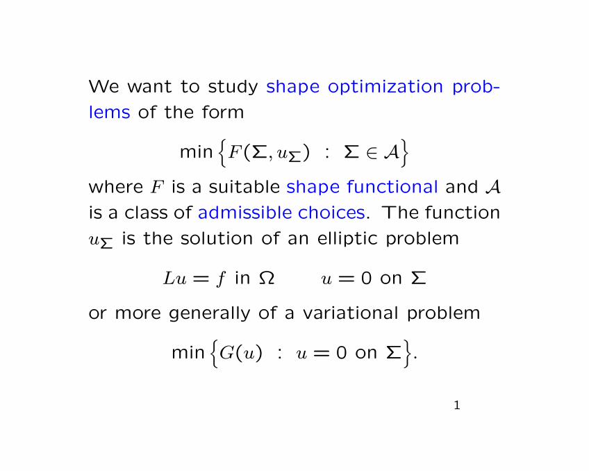
We want to study shape optimization prob-

lems of the form

minF (Σ, uΣ) : Σ ∈ A

where F is a suitable shape functional and Ais a class of admissible choices. The function

uΣ is the solution of an elliptic problem

Lu = f in Ω u = 0 on Σ

or more generally of a variational problem

minG(u) : u = 0 on Σ

.

1

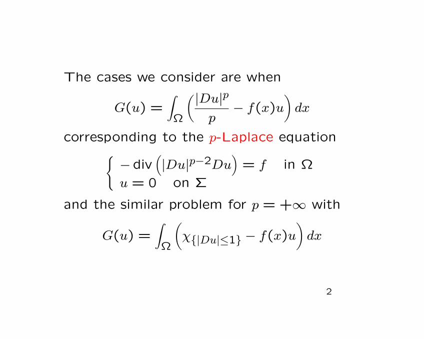
The cases we consider are when

G(u) =∫Ω

(|Du|p

p− f(x)u

)dx

corresponding to the p-Laplace equation−div

(|Du|p−2Du

)= f in Ω

u = 0 on Σ

and the similar problem for p = +∞ with

G(u) =∫Ω

(χ|Du|≤1 − f(x)u

)dx

2

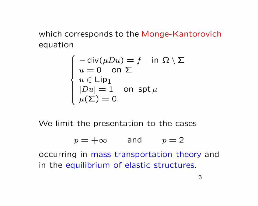
which corresponds to the Monge-Kantorovich

equation

−div(µDu) = f in Ω \Σu = 0 on Σu ∈ Lip1|Du| = 1 on sptµµ(Σ) = 0.

We limit the presentation to the cases

p = +∞ and p = 2

occurring in mass transportation theory and

in the equilibrium of elastic structures.

3

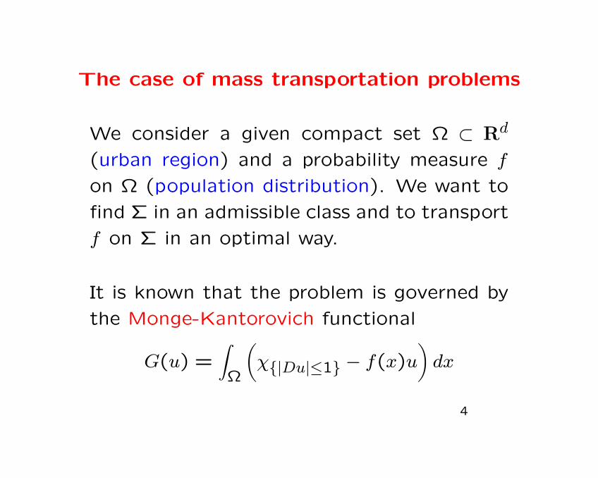
The case of mass transportation problems

We consider a given compact set Ω ⊂ Rd

(urban region) and a probability measure f

on Ω (population distribution). We want to

find Σ in an admissible class and to transport

f on Σ in an optimal way.

It is known that the problem is governed by

the Monge-Kantorovich functional

G(u) =∫Ω

(χ|Du|≤1 − f(x)u

)dx

4

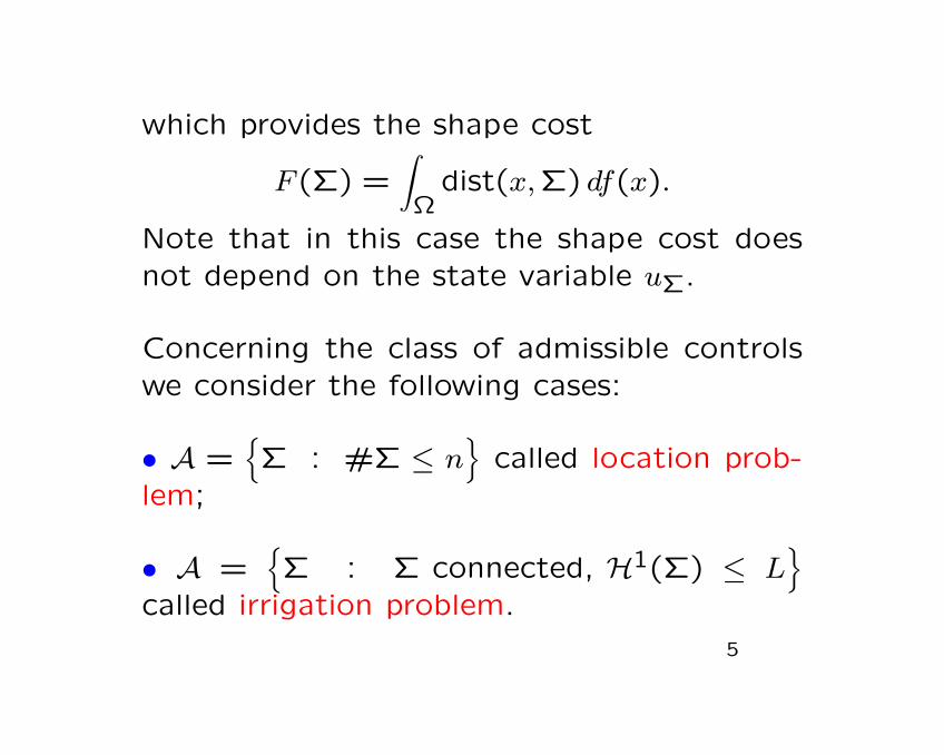
which provides the shape cost

F (Σ) =∫Ω

dist(x,Σ) df(x).

Note that in this case the shape cost doesnot depend on the state variable uΣ.

Concerning the class of admissible controlswe consider the following cases:

• A =Σ : #Σ ≤ n

called location prob-

lem;

• A =Σ : Σ connected, H1(Σ) ≤ L

called irrigation problem.

5

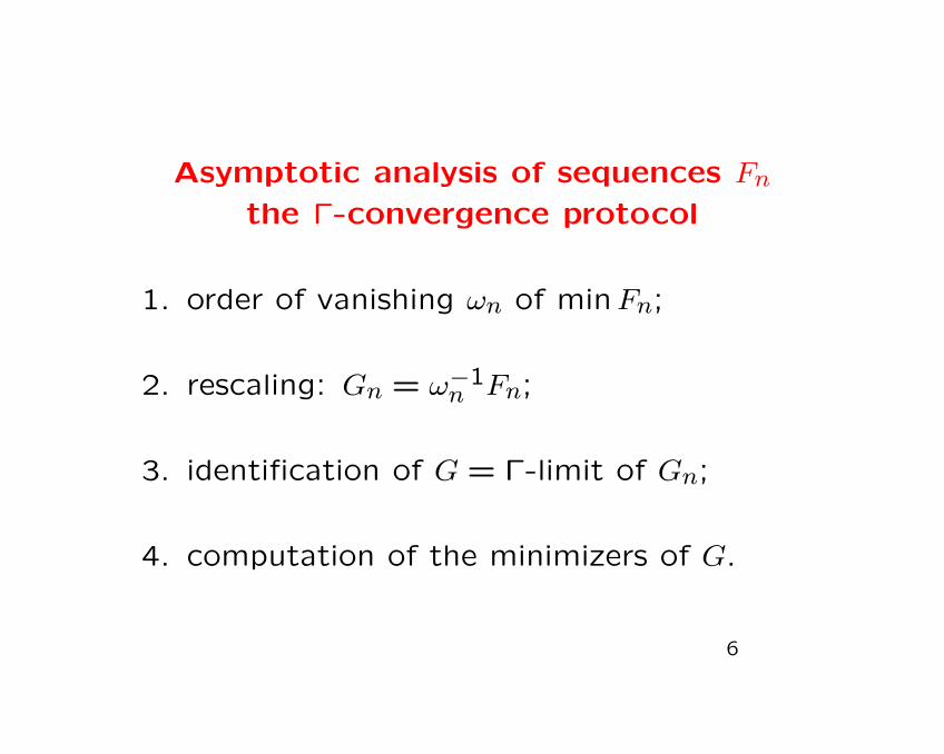
Asymptotic analysis of sequences Fn

the Γ-convergence protocol

1. order of vanishing ωn of minFn;

2. rescaling: Gn = ω−1n Fn;

3. identification of G = Γ-limit of Gn;

4. computation of the minimizers of G.

6

The location problem

We call optimal location problem the mini-mization problem

Ln = minF (Σ) : Σ ⊂ Ω, #Σ ≤ n

.

It has been extensively studied, see for in-stance

Suzuki, Asami, Okabe: Math. Program. 1991Suzuki, Drezner: Location Science 1996Buttazzo, Oudet, Stepanov: Birkhauser 2002Bouchitte, Jimenez, Rajesh: CRAS 2002Morgan, Bolton: Amer. Math. Monthly 2002. . . . . . . . .

7

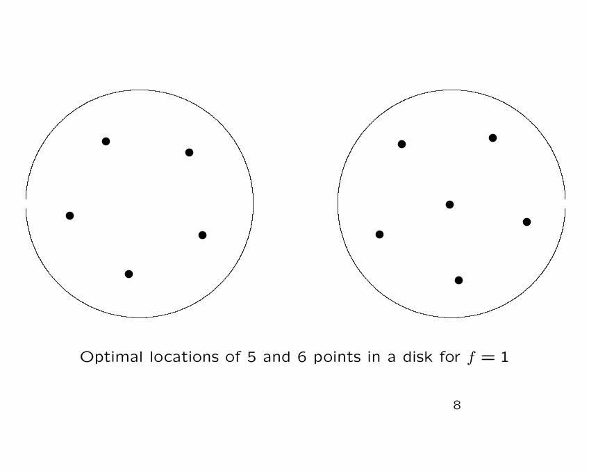
Optimal locations of 5 and 6 points in a disk for f = 1

8

We recall here the main known facts.

• Ln ≈ n−1/d as n → +∞;

• n1/dFn → Cd

∫Ω

µ−1/df(x) dx as n → +∞, in

the sense of Γ-convergence, where the limitfunctional is defined on probability measures;

• µopt = Kdfd/(1+d) hence the optimal con-

figurations Σn are asymptotically distributedin Ω as fd/(1+d) and not as f (for instanceas f2/3 in dimension two).

• in dimension two the optimal configurationapproaches the one given by the centers ofregular exagons.

9

• In dimension one we have C1 = 1/4.

• In dimension two we have

C2 =∫E|x| dx =

3 log3 + 4

6√

233/4≈ 0.377

where E is the regular hexagon of unit area

centered at the origin.

• If d ≥ 3 the value of Cd is not known.

• If d ≥ 3 the optimal asymptotical configu-

ration of the points is not known.

• The numerical computation of optimal con-

figurations is very heavy.

10

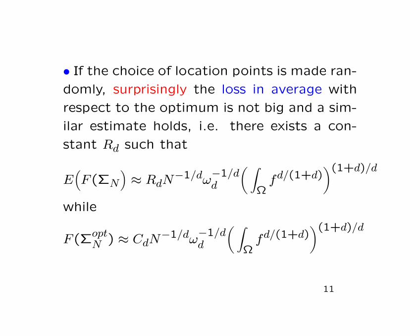
• If the choice of location points is made ran-

domly, surprisingly the loss in average with

respect to the optimum is not big and a sim-

ilar estimate holds, i.e. there exists a con-

stant Rd such that

E(F (ΣN

)≈ RdN

−1/dω−1/dd

( ∫Ω

fd/(1+d))(1+d)/d

while

F (ΣoptN ) ≈ CdN

−1/dω−1/dd

( ∫Ω

fd/(1+d))(1+d)/d

11

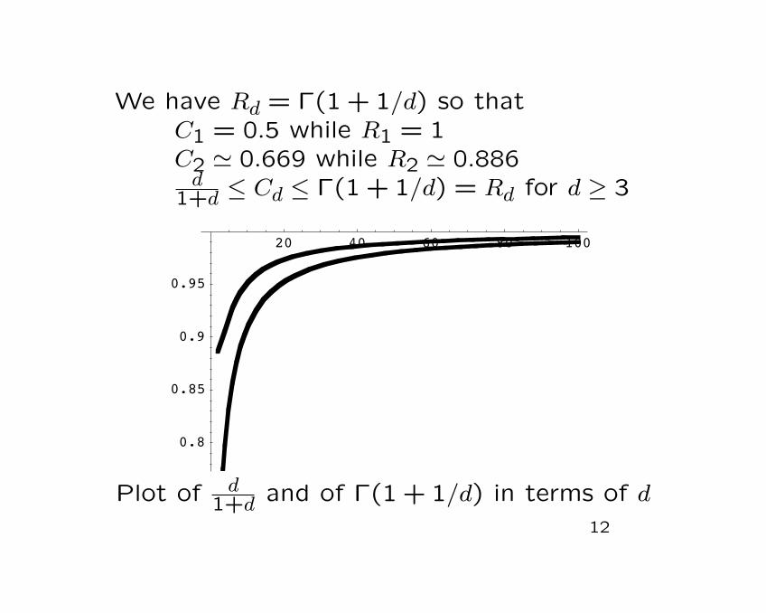
We have Rd = Γ(1 + 1/d) so thatC1 = 0.5 while R1 = 1C2 ' 0.669 while R2 ' 0.886

d1+d ≤ Cd ≤ Γ(1 + 1/d) = Rd for d ≥ 3

20 40 60 80 100

0.8

0.85

0.9

0.95

Untitled-1 1

Plot of d1+d and of Γ(1 + 1/d) in terms of d

12

The irrigation problem

Taking again the cost functional

F (Σ) :=∫Ω

dist(x,Σ) f(x) dx.

we consider the minimization problem

minF (Σ) : Σ connected, H1(Σ) ≤ `

Connected onedimensional subsets Σ of Ωare called networks.

Theorem For every ` > 0 there exists an op-timal network Σ` for the optimization prob-lem above.

13

Some necessary conditions of optimality on

Σ` have been derived:

Buttazzo-Oudet-Stepanov 2002,Buttazzo-Stepanov 2003,Santambrogio-Tilli 2005Mosconi-Tilli 2005.........

For instance the following facts have been

proved:

14

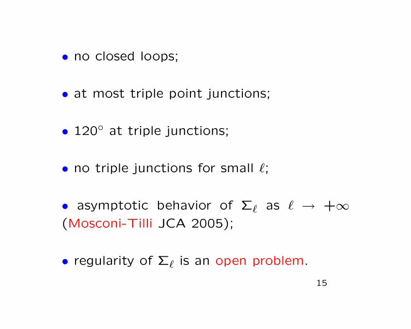
• no closed loops;

• at most triple point junctions;

• 120 at triple junctions;

• no triple junctions for small `;

• asymptotic behavior of Σ` as ` → +∞(Mosconi-Tilli JCA 2005);

• regularity of Σ` is an open problem.

15

Optimal sets of length 0.5 and 1 in a unit square with f = 1.

16

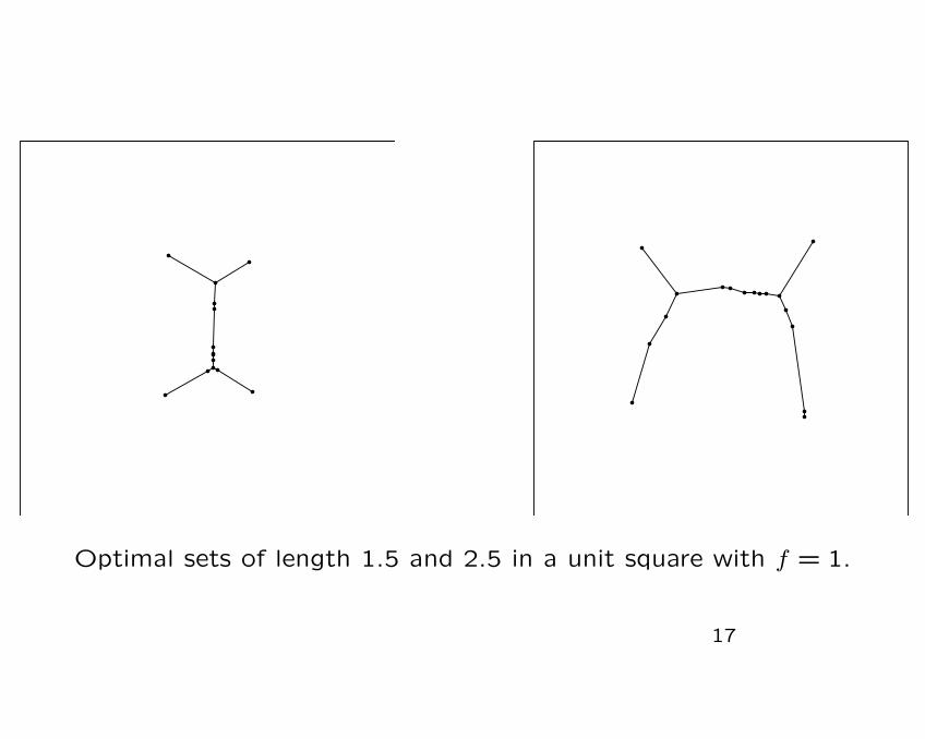
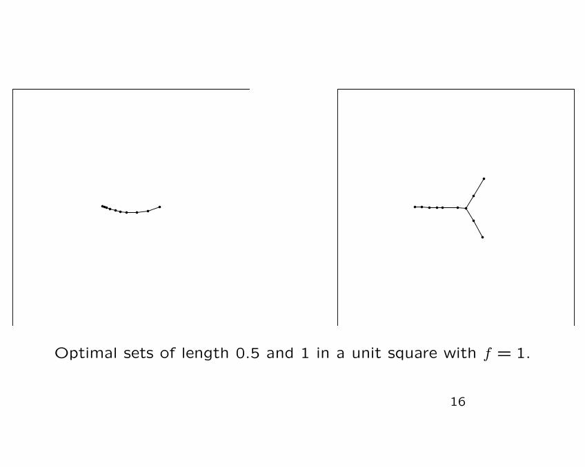
Optimal sets of length 1.5 and 2.5 in a unit square with f = 1.

17

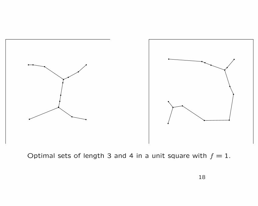
Optimal sets of length 3 and 4 in a unit square with f = 1.

18

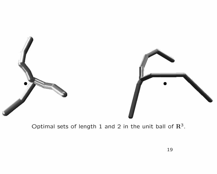
Optimal sets of length 1 and 2 in the unit ball of R3.

19

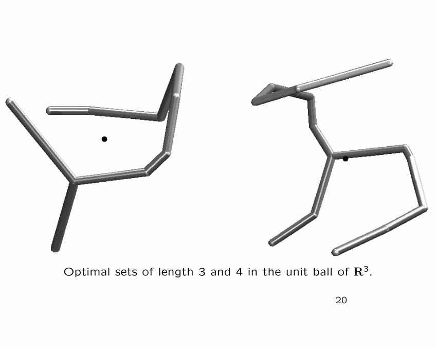
Optimal sets of length 3 and 4 in the unit ball of R3.

20

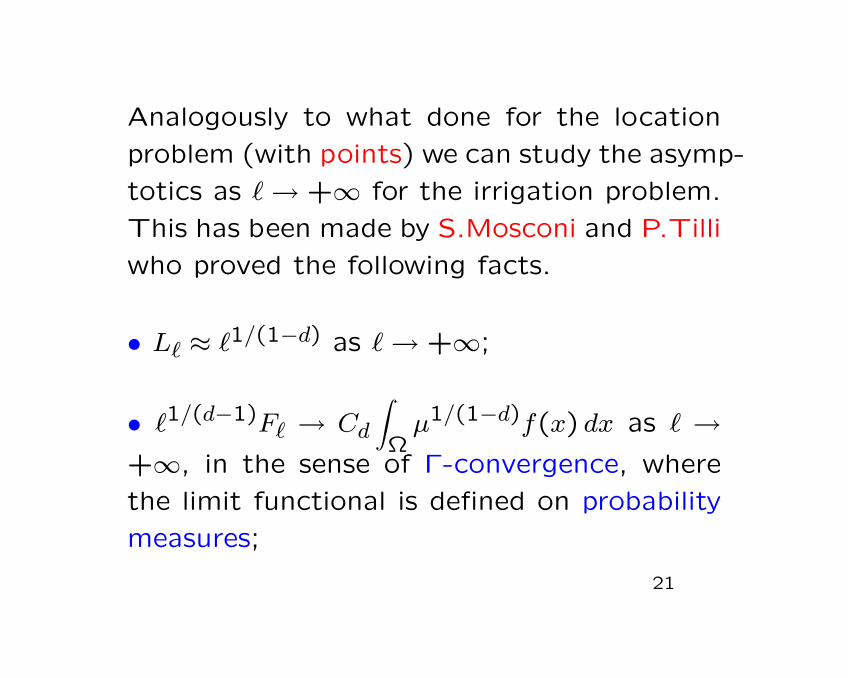
Analogously to what done for the location

problem (with points) we can study the asymp-

totics as ` → +∞ for the irrigation problem.

This has been made by S.Mosconi and P.Tilli

who proved the following facts.

• L` ≈ `1/(1−d) as ` → +∞;

• `1/(d−1)F` → Cd

∫Ω

µ1/(1−d)f(x) dx as ` →+∞, in the sense of Γ-convergence, where

the limit functional is defined on probability

measures;

21

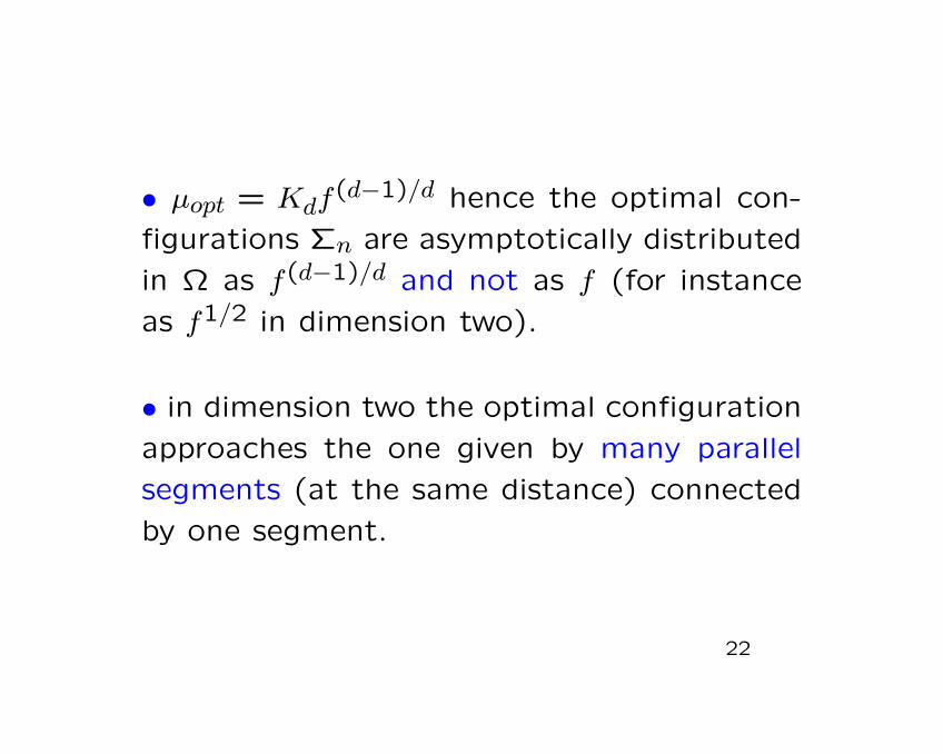
• µopt = Kdf(d−1)/d hence the optimal con-

figurations Σn are asymptotically distributed

in Ω as f(d−1)/d and not as f (for instance

as f1/2 in dimension two).

• in dimension two the optimal configuration

approaches the one given by many parallel

segments (at the same distance) connected

by one segment.

22

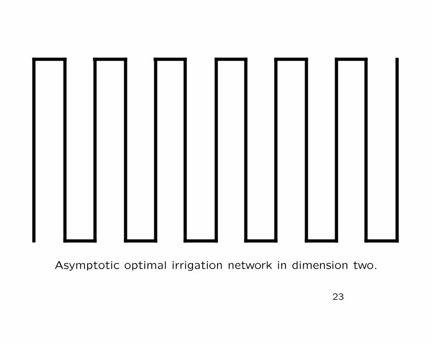
Asymptotic optimal irrigation network in dimension two.

23

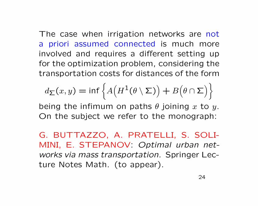
The case when irrigation networks are nota priori assumed connected is much moreinvolved and requires a different setting upfor the optimization problem, considering thetransportation costs for distances of the form

dΣ(x, y) = infA

(H1(θ \Σ)

)+ B

(θ ∩Σ

)being the infimum on paths θ joining x to y.On the subject we refer to the monograph:

G. BUTTAZZO, A. PRATELLI, S. SOLI-MINI, E. STEPANOV: Optimal urban net-works via mass transportation. Springer Lec-ture Notes Math. (to appear).

24

The case of elastic compliance

The goal is to study the configurations thatprovide the minimal compliance of a struc-ture. We want to find the optimal regionwhere to clamp a structure in order to ob-tain the highest rigidity.

The class of admissible choices may be, asin the case of mass transportation, a set ofpoints or a one-dimensional connected set.

Think for instance to the problem of locat-ing in an optimal way (for the elastic com-pliance) the six legs of a table, as below.

25

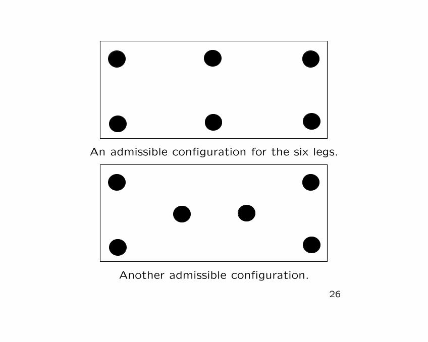
An admissible configuration for the six legs.

Another admissible configuration.

26

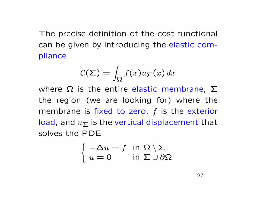
The precise definition of the cost functional

can be given by introducing the elastic com-

pliance

C(Σ) =∫Ω

f(x)uΣ(x) dx

where Ω is the entire elastic membrane, Σ

the region (we are looking for) where the

membrane is fixed to zero, f is the exterior

load, and uΣ is the vertical displacement that

solves the PDE−∆u = f in Ω \Σu = 0 in Σ ∪ ∂Ω

27

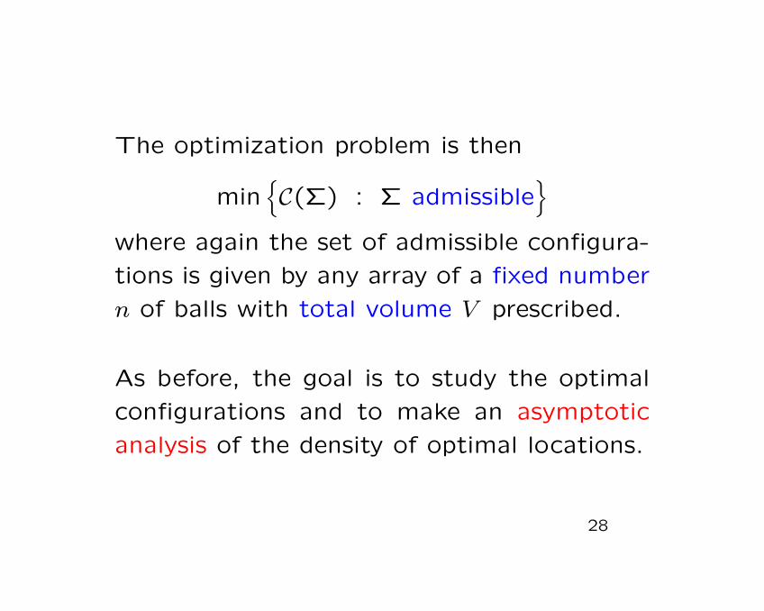
The optimization problem is then

minC(Σ) : Σ admissible

where again the set of admissible configura-

tions is given by any array of a fixed number

n of balls with total volume V prescribed.

As before, the goal is to study the optimal

configurations and to make an asymptotic

analysis of the density of optimal locations.

28

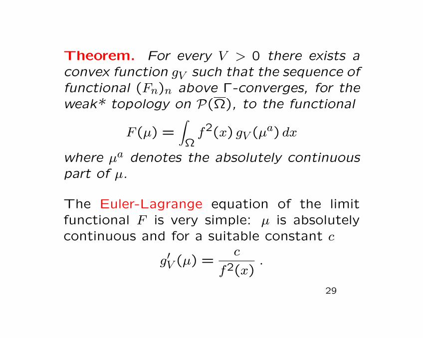
Theorem. For every V > 0 there exists aconvex function gV such that the sequence offunctional (Fn)n above Γ-converges, for theweak* topology on P(Ω), to the functional

F (µ) =∫Ω

f2(x) gV (µa) dx

where µa denotes the absolutely continuouspart of µ.

The Euler-Lagrange equation of the limitfunctional F is very simple: µ is absolutelycontinuous and for a suitable constant c

g′V (µ) =c

f2(x).

29

Open problems

• Exagonal tiling for f = 1?

• Non-circular regions Σ, where also the ori-

entation should appear in the limit.

• Computation of the limit function gV .

• Quasistatic evolution, when the points are

added one by one, without modifying the

ones that are already located.

30

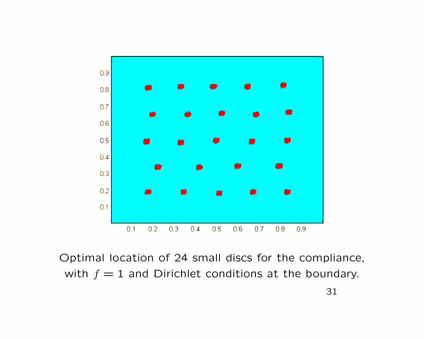
Optimal location of 24 small discs for the compliance,

with f = 1 and Dirichlet conditions at the boundary.

31

Optimal location of many small discs for the compliance,

with f = 1 and periodic conditions at the boundary.

32

Optimal compliance networks

We consider the problem of finding the bestlocation of a Dirichlet region Σ for a two-dimensional membrane Ω subjected to a givenvertical force f . The admissible Σ belong tothe class of all closed connected subsets ofΩ with H1(Σ) ≤ L.

The existence of an optimal configurationΣL for the optimization problem describedabove is well known; for instance it can beseen as a consequence of the Sverak com-pactness result.

33

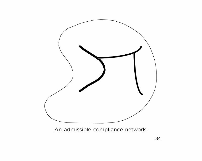
An admissible compliance network.

34

As in the previous situations we are inter-

ested in the asymptotic behaviour of ΣL as

L → +∞; more precisely our goal is to obtain

the limit distribution (density of lenght per

unit area) of ΣL as a limit probability mea-

sure that minimize the Γ-limit functional of

the suitably rescaled compliances.

To do this it is convenient to associate to

every Σ the probability measure

µΣ =H1xΣ

H1(Σ)

35

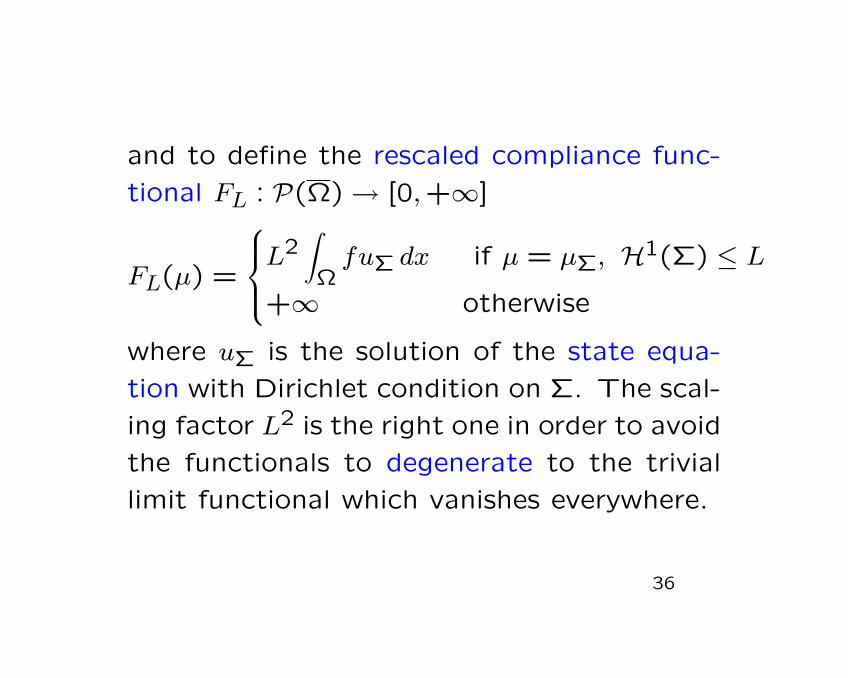
and to define the rescaled compliance func-

tional FL : P(Ω) → [0,+∞]

FL(µ) =

L2∫Ω

fuΣ dx if µ = µΣ, H1(Σ) ≤ L

+∞ otherwise

where uΣ is the solution of the state equa-

tion with Dirichlet condition on Σ. The scal-

ing factor L2 is the right one in order to avoid

the functionals to degenerate to the trivial

limit functional which vanishes everywhere.

36

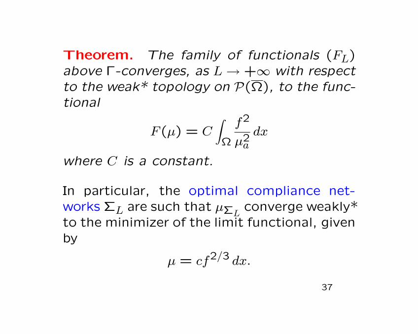
Theorem. The family of functionals (FL)above Γ-converges, as L → +∞ with respectto the weak* topology on P(Ω), to the func-tional

F (µ) = C∫Ω

f2

µ2a

dx

where C is a constant.

In particular, the optimal compliance net-works ΣL are such that µΣL

converge weakly*to the minimizer of the limit functional, givenby

µ = cf2/3 dx.

37

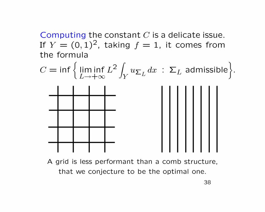
Computing the constant C is a delicate issue.If Y = (0,1)2, taking f = 1, it comes fromthe formula

C = inf

lim infL→+∞

L2∫Y

uΣLdx : ΣL admissible

.

A grid is less performant than a comb structure,

that we conjecture to be the optimal one.

38

Open problems

• Optimal periodic network for f = 1? Thiswould give the value of the constant C.

• Numerical computation of the optimal net-works ΣL.

• Quasistatic evolution, when the length in-creases with the time and ΣL also increaseswith respect to the inclusion (irreversibility).

• Same analysis with −∆p, and limit be-haviour as p → +∞, to see if the geometricproblem of average distance can be recov-ered.

39

References

G. Bouchitte, C. Jimenez, M. Rajesh CRAS

2002.

G. Buttazzo, F. Santambrogio, N. Varchon

COCV 2006, http://cvgmt.sns.it

F. Morgan, R. Bolton Amer. Math. Monthly

2002.

S. Mosconi, P. Tilli J. Conv. Anal. 2005,

http://cvgmt.sns.it

G. Buttazzo, F. Santambrogio NHM 2007,

http://cvgmt.sns.it.

40