CS340 Machine learningBayesian statistics 1

Fundamental principle of Bayesian statistics

• In Bayesian stats, everything that is uncertain (e.g., θ) is modeled with a probability distribution.

• We incorporate everything that is known (e.g., D) is by conditioning on it, using Bayes rule to update our prior beliefs into posterior beliefs.

p(θ|D) ∝ p(θ)p(D|θ)

In praise of Bayes

• Bayesian methods are conceptually simple and elegant, and can handle small sample sizes (e.g., one-shot learning) and complex hierarchical models without overfitting.

• They provide a single mechanism for answering all questions of interest; there is no need to choose between different estimators, hypothesis testing procedures, etc.

• They avoid various pathologies associated with orthodox statistics.

• They often enjoy good frequentist properties.

Why isn’t everyone a Bayesian?

• The need for a prior.

• Computational issues.

The need for a prior

• Bayes rule requires a prior, which is considered “subjective”.

• However, we know learning without assumptions is impossible (no free lunch theorem).

• Often we actually have informative prior knowledge.• If not, it is possible to create relatively

“uninformative” priors to represent prior ignorance.

• We can also estimate our priors from data (empirical Bayes).

• We can use posterior predictive checks to test goodness of fit of both prior and likelihood.

Computational issues

• Computing the normalization constant requires integrating over all the parameters

• Computing posterior expectations requires integrating over all the parameters

p(θ|D) =p(θ)p(D|θ)∫p(θ′)p(D|θ′)dθ′

Ef(Θ) =

∫f(θ)p(θ|D)dθ

Approximate inference

• We can evaluate posterior expectations using Monte Carlo integration

• Generating posterior samples can be tricky– Importance sampling– Particle filtering– Markov chain Monte Carlo (MCMC)

• There are also deterministic approximation methods– Laplace– Variational Bayes– Expectation Propagation

Ef(Θ) =

∫f(θ)p(θ|D)dθ ≈

1

N

N∑

s=1

f(θs) where θs ∼ p(θ|D)

Not on exam

Conjugate priors

• For simplicity, we will mostly focus on a special kind of prior which has nice mathematical properties.

• A prior p(θ) is said to be conjugate to a likelihood p(D|θ) if the corresponding posterior p(θ|D) has the same functional form as p(θ).

• This means the prior family is closed under Bayesian updating.

• So we can recursively apply the rule to update our beliefs as data streams in (online learning).

• A natural conjugate prior means p(θ) has the same functional form as p(D|θ).

Example: coin tossing

• Consider the problem of estimating the probability of heads θ from a sequence of N coin tosses, D = (X1, …, XN)

• First we define the likelihood function, then the prior, then compute the posterior. We will also consider different ways to predict the future.

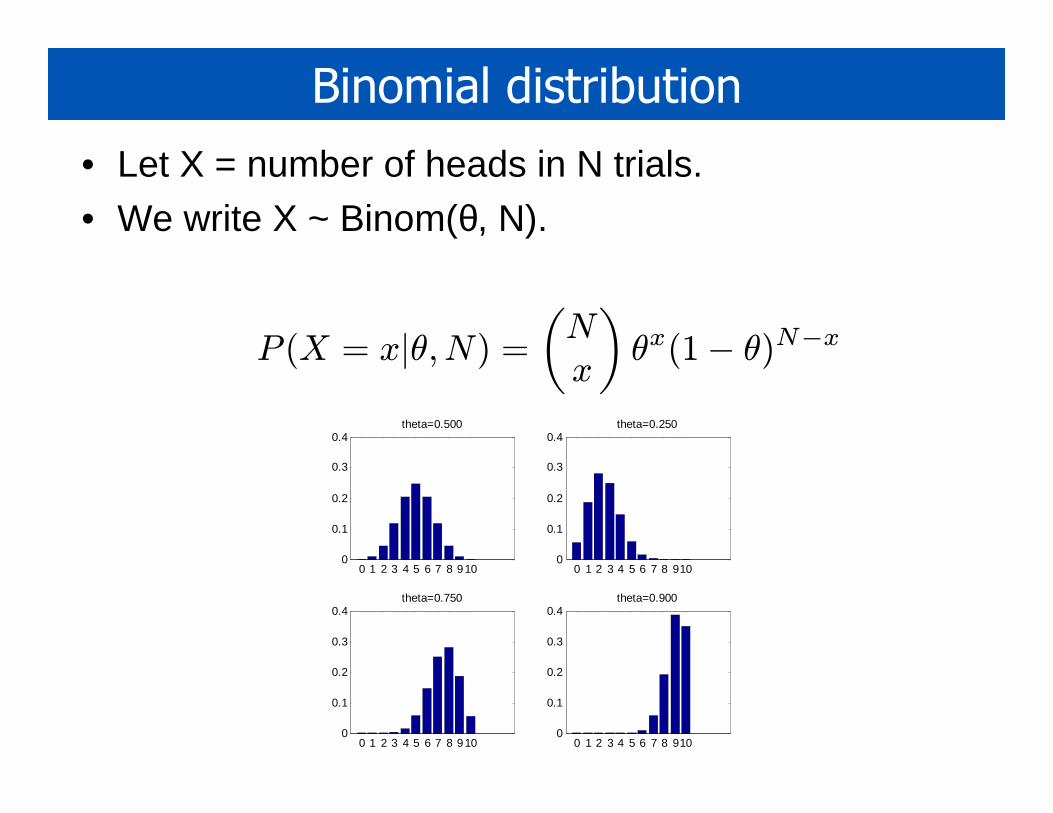
Binomial distribution

• Let X = number of heads in N trials.

• We write X ~ Binom(θ, N).

0 1 2 3 4 5 6 7 8 9100

0.1

0.2

0.3

0.4theta=0.500

0 1 2 3 4 5 6 7 8 9100

0.1

0.2

0.3

0.4theta=0.250

0 1 2 3 4 5 6 7 8 9100

0.1

0.2

0.3

0.4theta=0.750

0 1 2 3 4 5 6 7 8 9100

0.1

0.2

0.3

0.4theta=0.900

P (X = x|θ,N) =

(N

x

)θx(1− θ)N−x

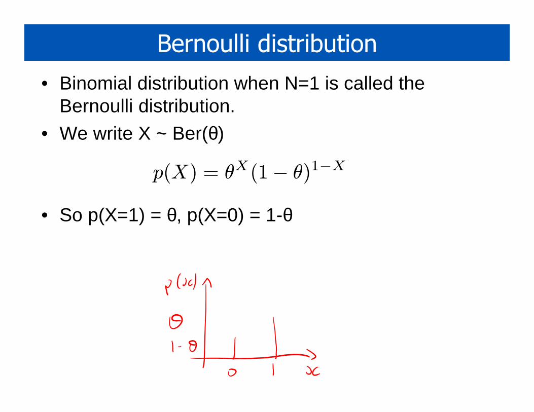
Bernoulli distribution

• Binomial distribution when N=1 is called the Bernoulli distribution.

• We write X ~ Ber(θ)

• So p(X=1) = θ, p(X=0) = 1-θ

p(X) = θX(1− θ)1−X

Fitting a Bernoulli distribution

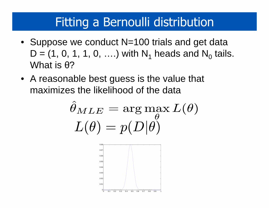
• Suppose we conduct N=100 trials and get data D = (1, 0, 1, 1, 0, ….) with N1 heads and N0 tails. What is θ?

• A reasonable best guess is the value that maximizes the likelihood of the data

0 0.1 0.2 0.3 0.4 0.5 0.6 0.7 0.8 0.9 10

0.01

0.02

0.03

0.04

0.05

0.06

0.07

0.08

θ̂MLE = argmaxθ

L(θ)

L(θ) = p(D|θ)

Bernoulli likelihood function

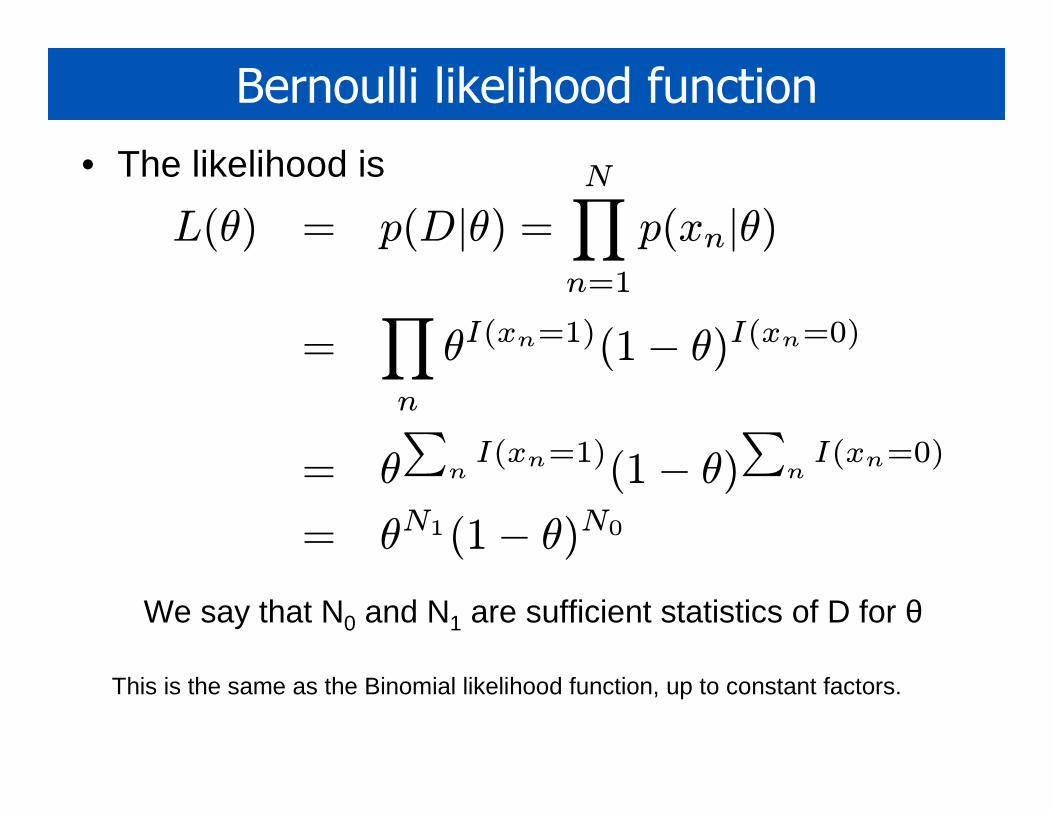
• The likelihood is

L(θ) = p(D|θ) =N∏

n=1

p(xn|θ)

=∏

n

θI(xn=1)(1− θ)I(xn=0)

= θ

∑nI(xn=1)(1− θ)

∑nI(xn=0)

= θN1(1− θ)N0

We say that N0 and N1 are sufficient statistics of D for θ

This is the same as the Binomial likelihood function, up to constant factors.

Bernoulli log-likelihood

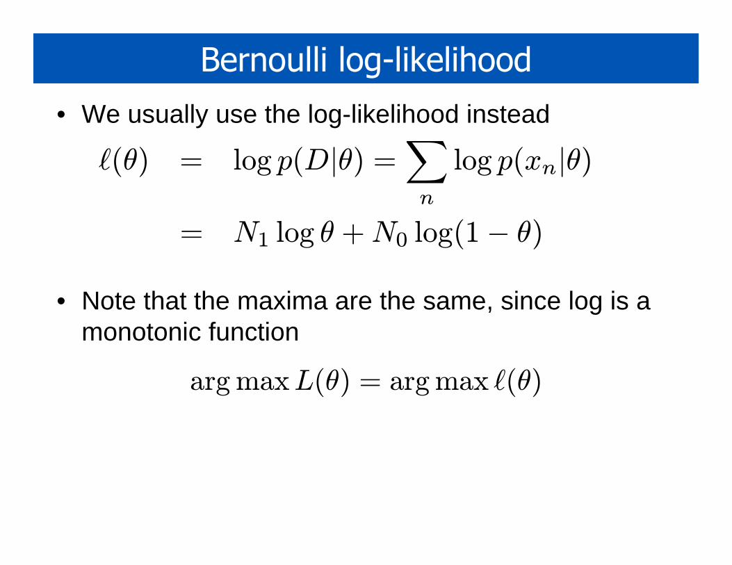
• We usually use the log-likelihood instead

• Note that the maxima are the same, since log is a monotonic function

argmaxL(θ) = argmax ℓ(θ)

ℓ(θ) = log p(D|θ) =∑

n

log p(xn|θ)

= N1 log θ +N0 log(1− θ)

Computing the Bernoulli MLE

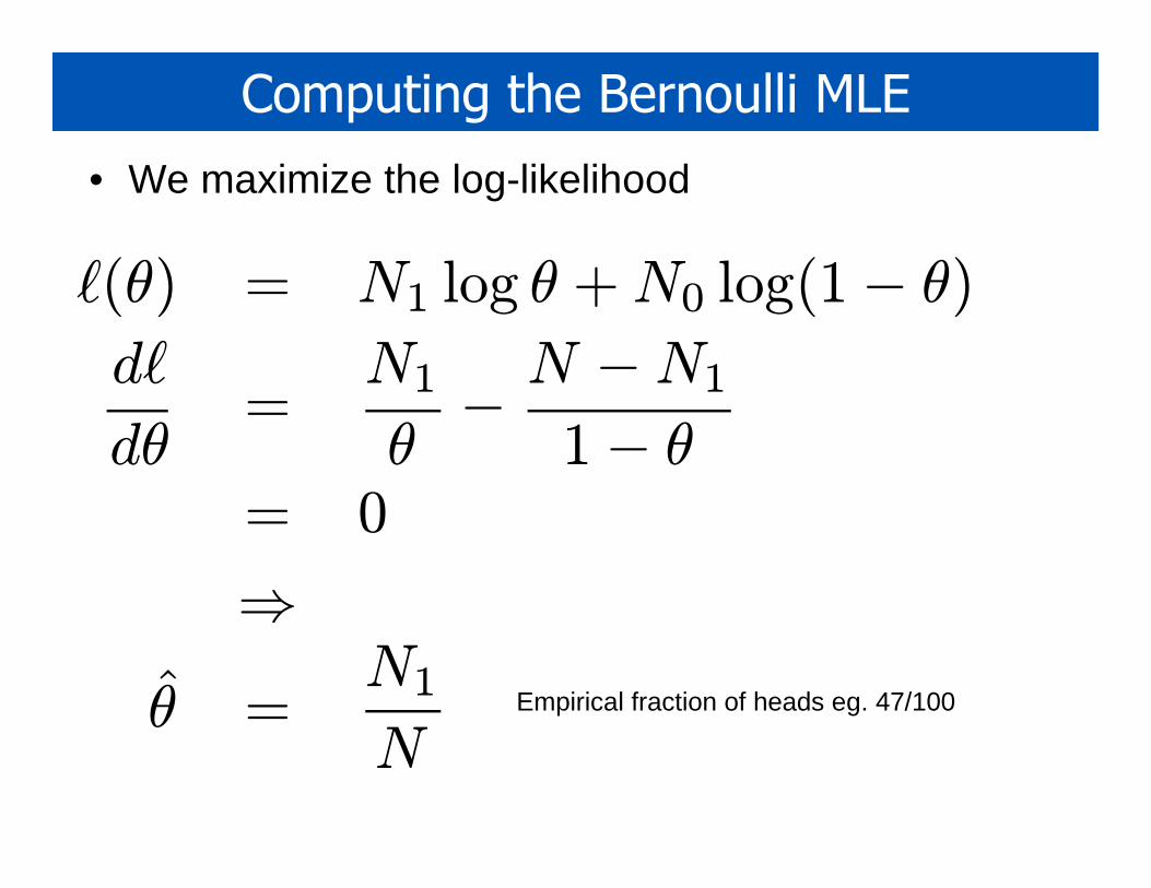
• We maximize the log-likelihood

ℓ(θ) = N1 log θ +N0 log(1− θ)

dℓ

dθ=

N1

θ−N −N11− θ

= 0

⇒

θ̂ =N1

NEmpirical fraction of heads eg. 47/100

Black swan paradox

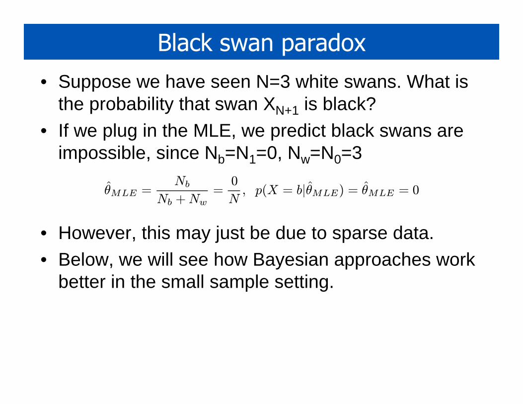
• Suppose we have seen N=3 white swans. What is the probability that swan XN+1 is black?

• If we plug in the MLE, we predict black swans are impossible, since Nb=N1=0, Nw=N0=3

• However, this may just be due to sparse data. • Below, we will see how Bayesian approaches work

better in the small sample setting.

θ̂MLE =Nb

Nb +Nw=0

N, p(X = b|θ̂MLE) = θ̂MLE = 0

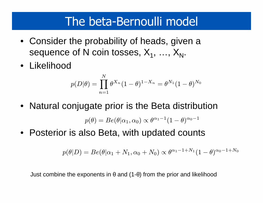
The beta-Bernoulli model

• Consider the probability of heads, given a sequence of N coin tosses, X1, …, XN.

• Likelihood

• Natural conjugate prior is the Beta distribution

• Posterior is also Beta, with updated counts

p(D|θ) =N∏

n=1

θXn(1− θ)1−Xn = θN1(1− θ)N0

p(θ) = Be(θ|α1, α0) ∝ θα1−1(1− θ)α0−1

p(θ|D) = Be(θ|α1 +N1, α0 +N0) ∝ θα1−1+N1(1− θ)α0−1+N0

Just combine the exponents in θ and (1-θ) from the prior and likelihood

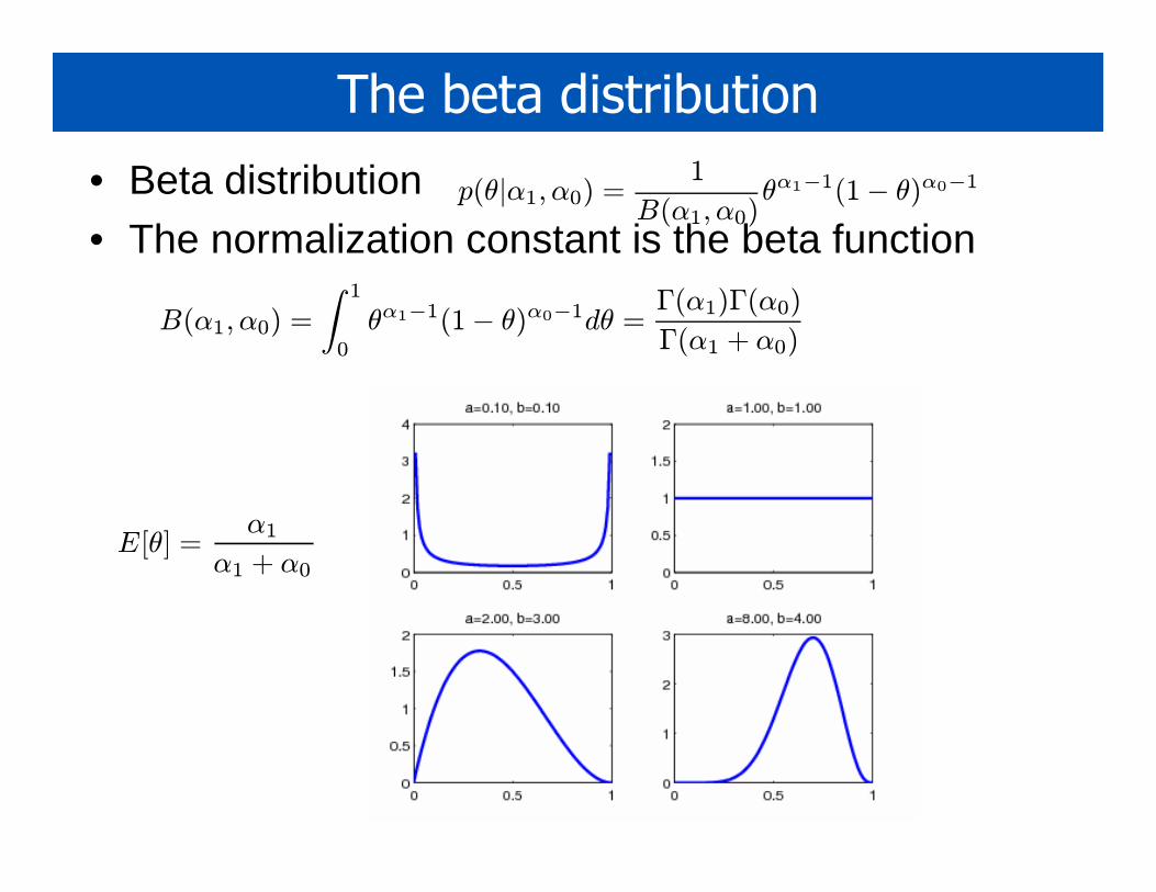
The beta distribution

• Beta distribution

• The normalization constant is the beta function p(θ|α1, α0) =

1

B(α1, α0)θα1−1(1− θ)α0−1

E[θ] =α1

α1 + α0

B(α1, α0) =

∫ 1

0

θα1−1(1− θ)α0−1dθ =Γ(α1)Γ(α0)

Γ(α1 + α0)

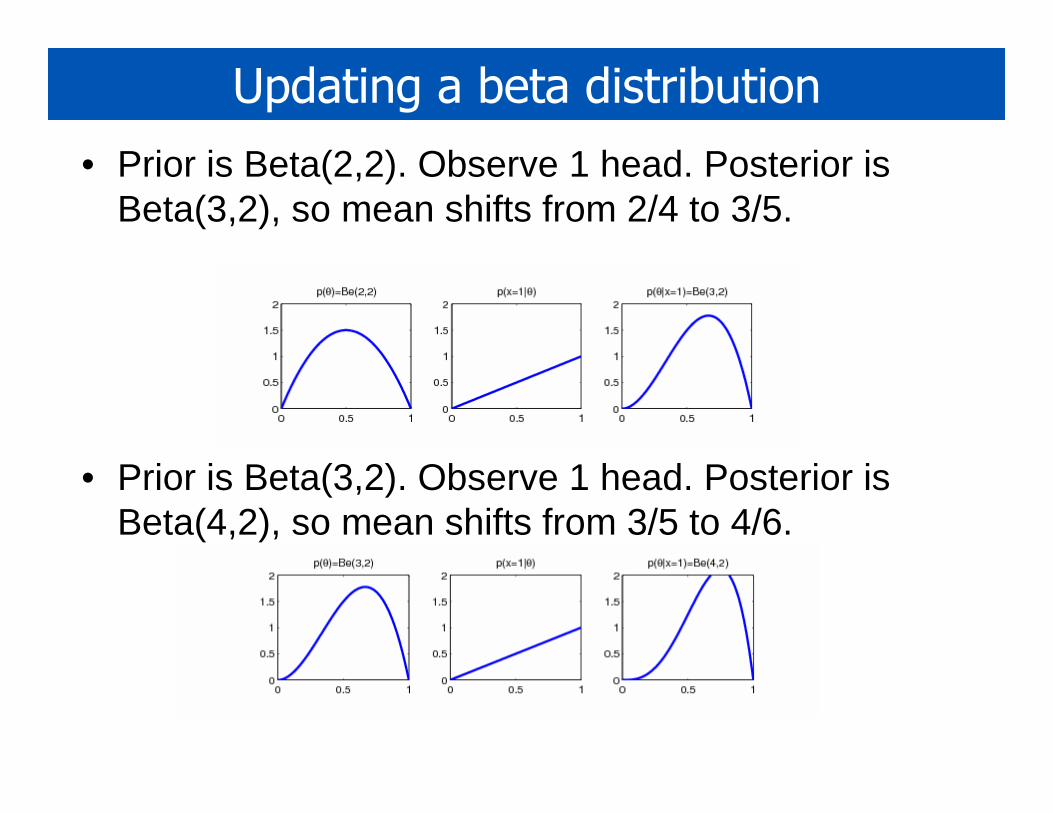
Updating a beta distribution

• Prior is Beta(2,2). Observe 1 head. Posterior is Beta(3,2), so mean shifts from 2/4 to 3/5.

• Prior is Beta(3,2). Observe 1 head. Posterior is Beta(4,2), so mean shifts from 3/5 to 4/6.

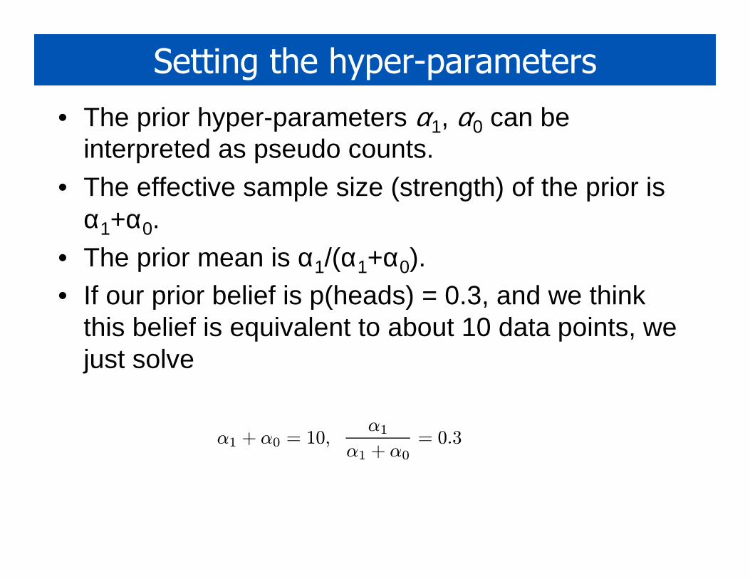
Setting the hyper-parameters

• The prior hyper-parameters α1, α0 can be interpreted as pseudo counts.

• The effective sample size (strength) of the prior is α1+α0.

• The prior mean is α1/(α1+α0).• If our prior belief is p(heads) = 0.3, and we think

this belief is equivalent to about 10 data points, we just solve

α1 + α0 = 10,α1

α1 + α0= 0.3

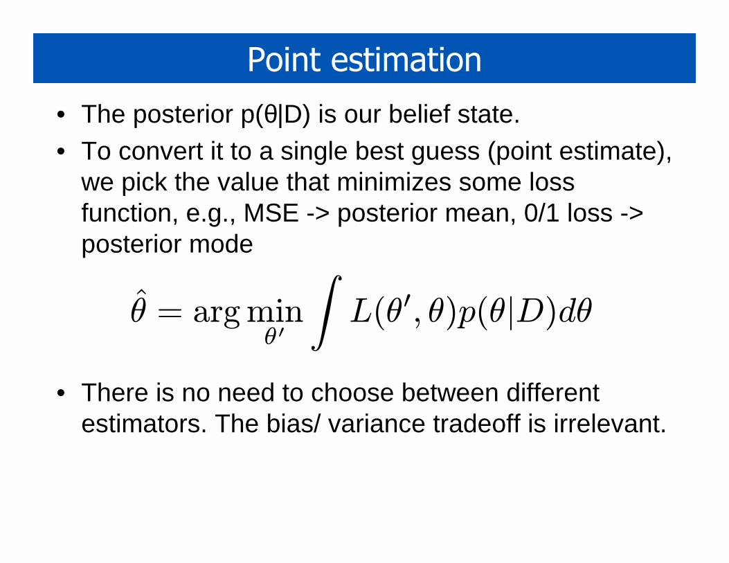
Point estimation

• The posterior p(θ|D) is our belief state.• To convert it to a single best guess (point estimate),

we pick the value that minimizes some loss function, e.g., MSE -> posterior mean, 0/1 loss -> posterior mode

• There is no need to choose between different estimators. The bias/ variance tradeoff is irrelevant.

θ̂ = argminθ′

∫L(θ′, θ)p(θ|D)dθ

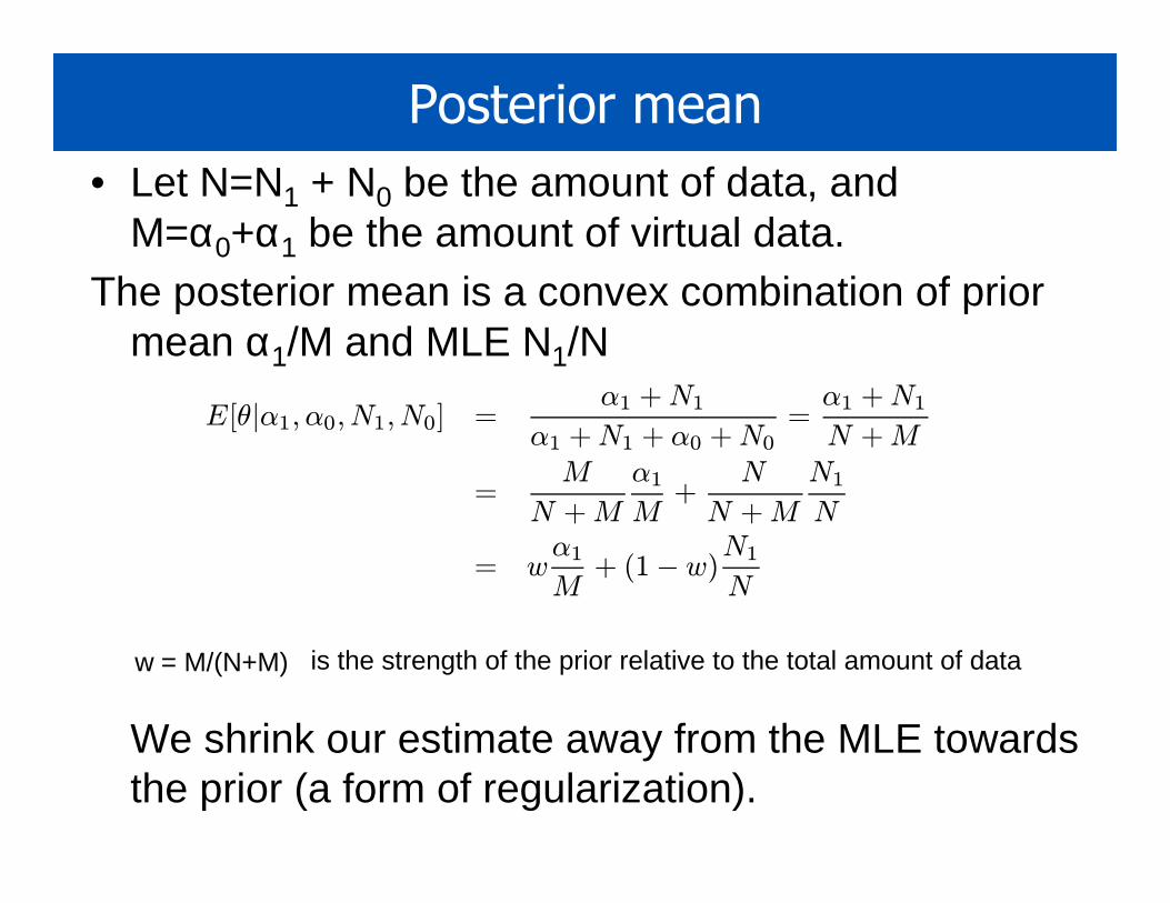
Posterior mean

• Let N=N1 + N0 be the amount of data, andM=α0+α1 be the amount of virtual data.

The posterior mean is a convex combination of prior mean α1/M and MLE N1/N

We shrink our estimate away from the MLE towards the prior (a form of regularization).

w = M/(N+M) is the strength of the prior relative to the total amount of data

E[θ|α1, α0, N1, N0] =α1 +N1

α1 +N1 + α0 +N0=α1 +N1N +M

=M

N +M

α1

M+

N

N +M

N1

N

= wα1

M+ (1− w)

N1

N

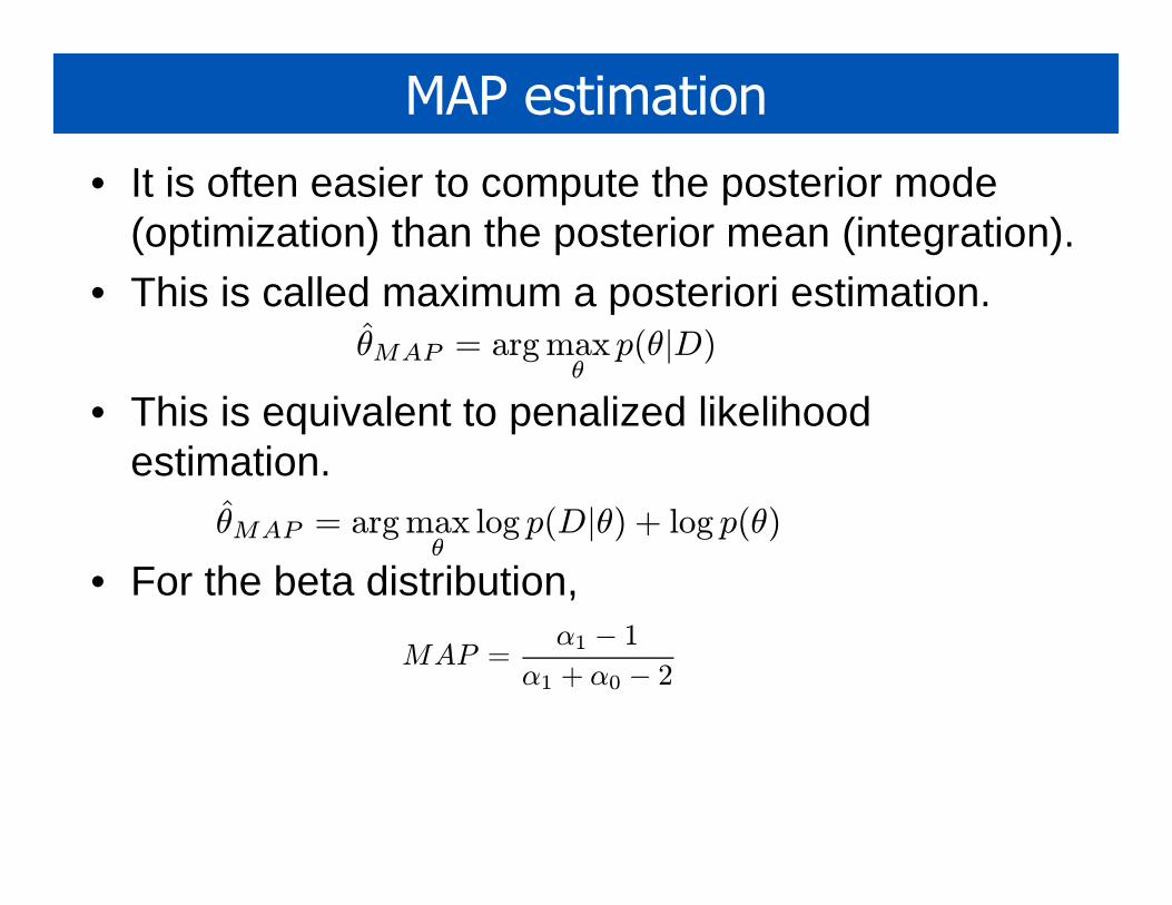
MAP estimation

• It is often easier to compute the posterior mode (optimization) than the posterior mean (integration).

• This is called maximum a posteriori estimation.

• This is equivalent to penalized likelihood estimation.

• For the beta distribution,

θ̂MAP = argmaxθ

p(θ|D)

θ̂MAP = argmaxθ

log p(D|θ) + log p(θ)

MAP =α1 − 1

α1 + α0 − 2

Posterior predictive distribution

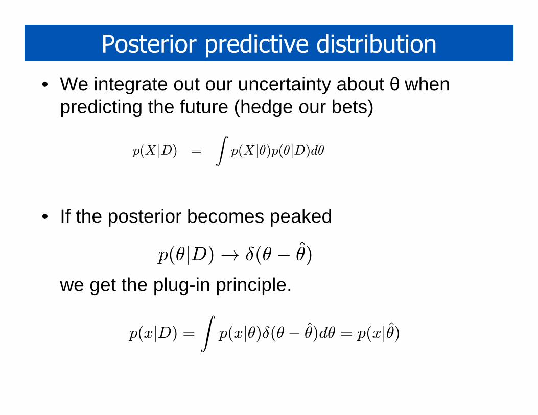
• We integrate out our uncertainty about θ when predicting the future (hedge our bets)

• If the posterior becomes peaked

we get the plug-in principle.

p(θ|D)→ δ(θ − θ̂)

p(X|D) =

∫p(X|θ)p(θ|D)dθ

p(x|D) =

∫p(x|θ)δ(θ − θ̂)dθ = p(x|θ̂)

Posterior predictive distribution

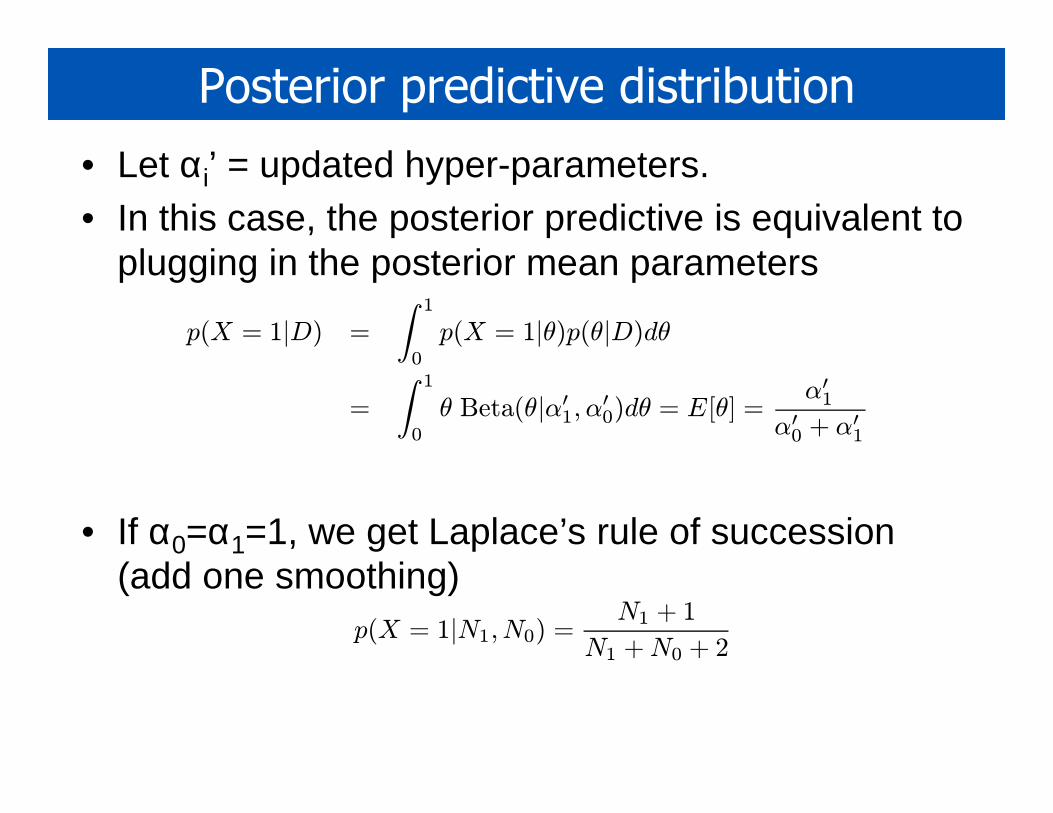
• Let αi’ = updated hyper-parameters.• In this case, the posterior predictive is equivalent to

plugging in the posterior mean parameters

• If α0=α1=1, we get Laplace’s rule of succession(add one smoothing)

p(X = 1|D) =

∫ 1

0

p(X = 1|θ)p(θ|D)dθ

=

∫ 1

0

θ Beta(θ|α′1, α′

0)dθ = E[θ] =α′1

α′0 + α′

1

p(X = 1|N1, N0) =N1 + 1

N1 +N0 + 2

Solution to black swan paradox

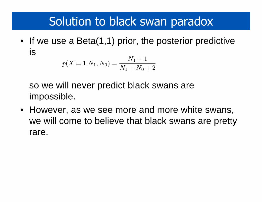
• If we use a Beta(1,1) prior, the posterior predictive is

so we will never predict black swans are impossible.

• However, as we see more and more white swans, we will come to believe that black swans are pretty rare.

p(X = 1|N1, N0) =N1 + 1

N1 +N0 + 2