
EXCEL DECISION MAKING TOOLS BASIC FORMULAE - REGRESSION - GOAL SEEK - SOLVER.
date post
21-Dec-2015Category
view
237download
1
Decision making as a model
6. A little bit of Bayesian statistics
0
0,1
0,2
0,3
0,4
0,5
0,6
0,7
0,8
0,9
1
0 0,2 0,4 0,6 0,8 1
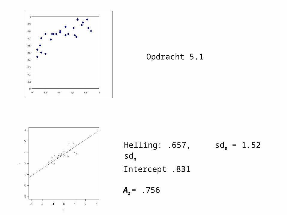
Helling: .657, sds = 1.52 sdn
Intercept .831
Az = .756
Opdracht 5.1

Opdracht 5.2
0
0,1
0,2
0,3
0,4
0,5
0,6
0,7
0,8
0,9
1
0 0,2 0,4 0,6 0,8 1
slope .643
Intercept 1.267
Az = .857
A B C D E
Prev. .75 .60 .25 .10 .06
d' 1.28 1.50 1.77 1.90 1.85
c -.44 -.19 .36 .70 .93
β .57 .76 1.89 3.75 5.57
βuneq .37 .49 1.22 2.41 3.58
LRopt .15 .31 1.37 4.11 7.16

N.B. a course on Bayesians statistics is impossible in one lecture
You might study:
-Bolstad, W.M. (2007). Introduction to Bayesian statistics, 2nd ed. Hoboken N.J. : Wiley.
-Gill, J. (2002). Bayesian methods: A social and behavioral approach. Boca Raton Fl: Chapman & Hall.
Or consult Herbert Hoijtink Irene Klugkist (M&T)
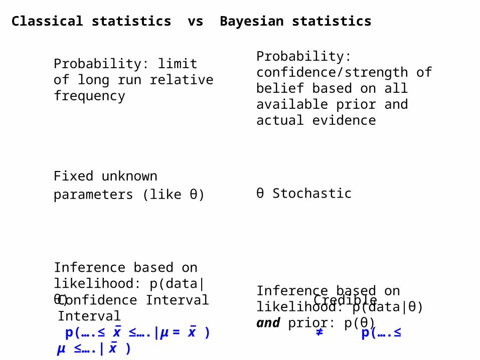
Classical statistics vs Bayesian statistics
Probability: limit of long run relative frequency
Fixed unknown parameters (like θ)
Inference based on likelihood: p(data|θ)
Probability: confidence/strength of belief based on all available prior and actual evidence
θ Stochastic
Inference based on likelihood: p(data|θ) and prior: p(θ)
Confidence Interval Credible Interval p(….≤ x̅� ≤….|μ = x̅� ) ≠ p(….≤ μ ≤….| x̅� )
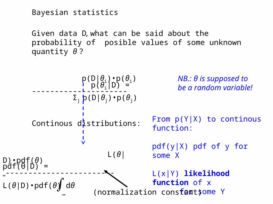
Given data D, what can be said about the probability of posible values of some unknown quantity θ ?
p(D|θi)•p(θi) p(θi|D) = ---------------------
Σj p(D|θj)•p(θj)
Continous distributions:
NB.: θ is supposed to be a random variable!
L(θ|D)•pdf(θ) pdf(θ|D) = ∞------------------------ L(θ|D)•pdf(θ) dθ
-∞
∫
Bayesian statistics
From p(Y|X) to continous function:
pdf(y|X) pdf of y for some X
L(x|Y) likelihood function of xfor some Y
(normalization constant)
0 0,1 0,2 0,3 0,4 0,5 0,6 0,7 0,8 0,9 1
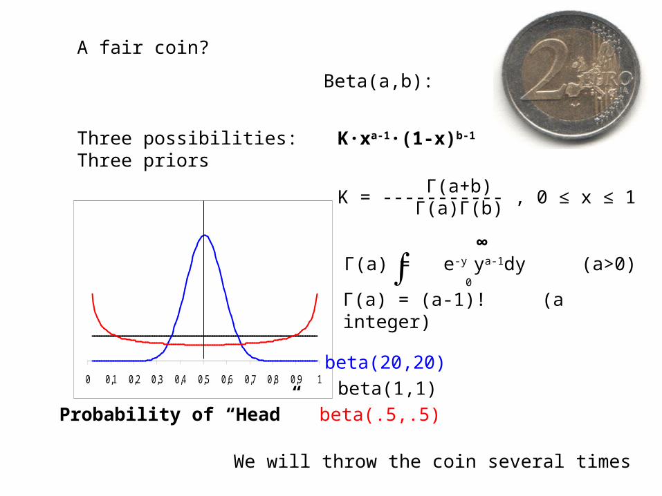
Probability of “Head”
Three possibilities:Three priors
A fair coin?
We will throw the coin several times
beta(20,20)
beta(1,1)
beta(.5,.5)
Beta(a,b):
K∙xa-1∙(1-x)b-1
Γ(a+b)K = ----------- , 0 ≤ x ≤ 1 Γ(a)Γ(b)
∞Γ(a) = e-y ya-1dy (a>0) 0∫Γ(a) = (a-1)! (a integer)
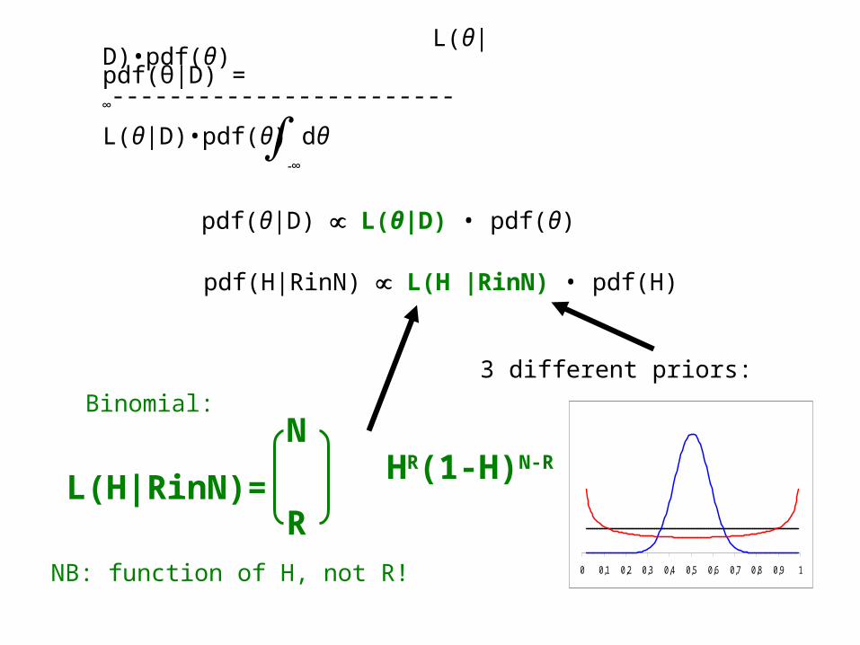
pdf(θ|D) L(θ|D) • pdf(θ)
N HR(1-H)N-R
R L(H|RinN)=
Binomial:
3 different priors:
0 0,1 0,2 0,3 0,4 0,5 0,6 0,7 0,8 0,9 1NB: function of H, not R!
pdf(H|RinN) L(H |RinN) • pdf(H)
L(θ|D)•pdf(θ) pdf(θ|D) = ∞------------------------ L(θ|D)•pdf(θ) dθ
-∞
∫
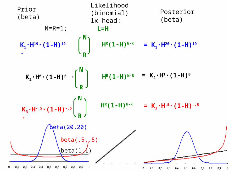
N HR(1-H)N-R
R
N HR(1-H)N-R
R
N HR(1-H)N-R
R
K1∙H19∙(1-H)19
∙
K2∙H0∙(1-H)0 ∙
K3∙H-.5∙(1-H)-.5 ∙
Prior (beta)Likelihood(binomial)
1x head: N=R=1; Posterior(beta)
= K1∙H20∙(1-H)19
= K2∙H1∙(1-H)0
= K3∙H.5∙(1-H)-.5
L=H
beta(20,20)
beta(.5,.5)
beta(1,1)
0 0,1 0,2 0,3 0,4 0,5 0,6 0,7 0,8 0,9 1
0 20 40 60 80 100
0 0,1 0,2 0,3 0,4 0,5 0,6 0,7 0,8 0,9 1
0 20 40 60 80 100
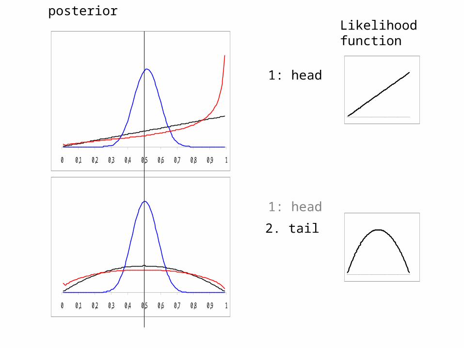
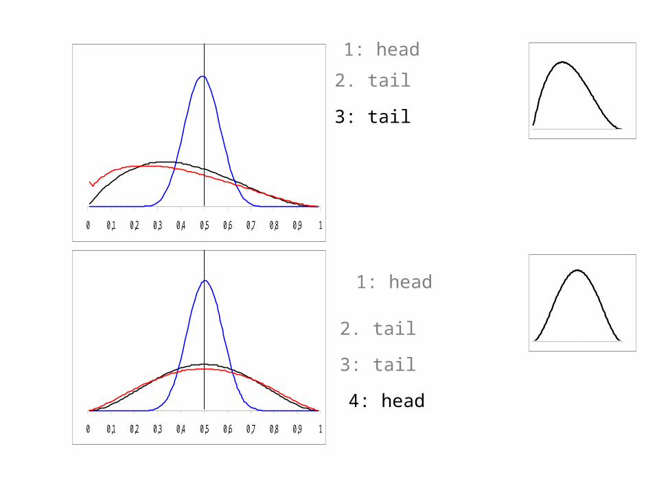
1: head
2. tail
Likelihoodfunction
posterior
1: head
0 0,1 0,2 0,3 0,4 0,5 0,6 0,7 0,8 0,9 1
0 20 40 60 80 100
0 0,1 0,2 0,3 0,4 0,5 0,6 0,7 0,8 0,9 1
0 20 40 60 80 100
3: tail
4: head
2. tail
1: head
3: tail
2. tail
1: head
0 0,1 0,2 0,3 0,4 0,5 0,6 0,7 0,8 0,9 1
0 20 40 60 80 100
0 0,1 0,2 0,3 0,4 0,5 0,6 0,7 0,8 0,9 1
0 20 40 60 80 100
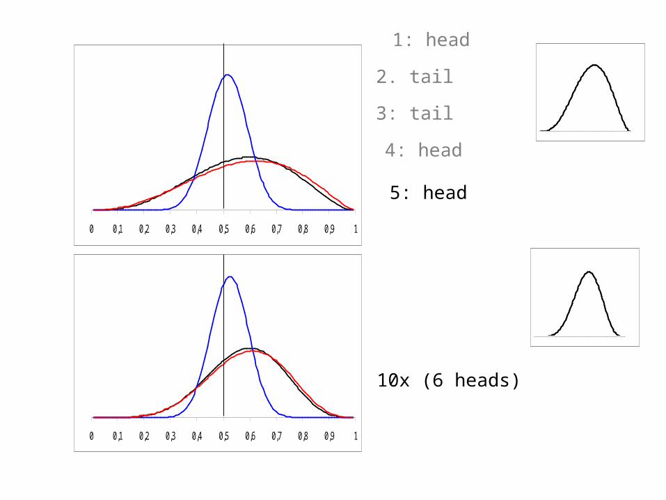
5: head
10x (6 heads)
4: head
3: tail
2. tail
1: head
0 0,1 0,2 0,3 0,4 0,5 0,6 0,7 0,8 0,9 1
0 20 40 60 80 100
0 0,1 0,2 0,3 0,4 0,5 0,6 0,7 0,8 0,9 1
0 20 40 60 80 100
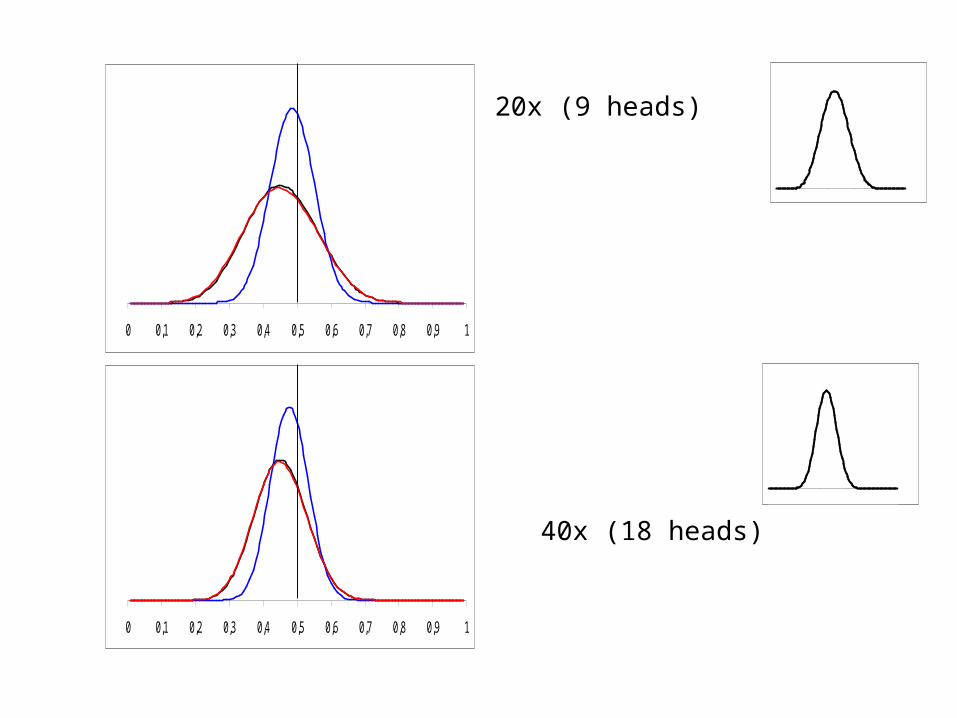
20x (9 heads)
40x (18 heads)
0 0,1 0,2 0,3 0,4 0,5 0,6 0,7 0,8 0,9 10 20 40 60 80 100
0 0,1 0,2 0,3 0,4 0,5 0,6 0,7 0,8 0,9 1
0 20 40 60 80 100
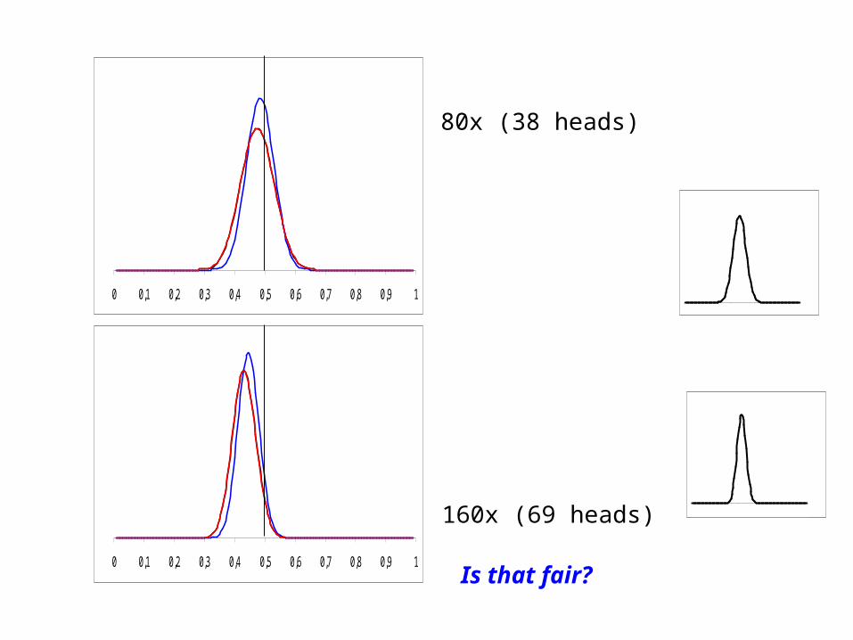
80x (38 heads)
160x (69 heads)
Is that fair?
0 0,1 0,2 0,3 0,4 0,5 0,6 0,7 0,8 0,9 1
0 20 40 60 80 100
0 0,1 0,2 0,3 0,4 0,5 0,6 0,7 0,8 0,9 1
0 20 40 60 80 100
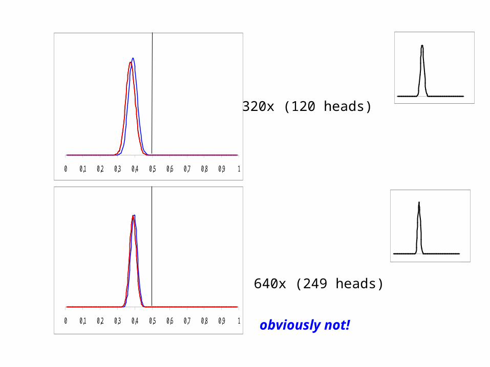
320x (120 heads)
640x (249 heads)
obviously not!
With lots of data the prior distribution does not make much difference anymore (although narrow priors retain their influence longer)
With fewer data the prior distribution does make a lot of difference, so you have to have good reasons for your prior distribution
This was an untypical case: the blue line prior was quite reasonable for coin-like objects, but this “coin” was a computer simulation (with H=.40)
Narrow priors distributions have strong influence on the posterior distribution
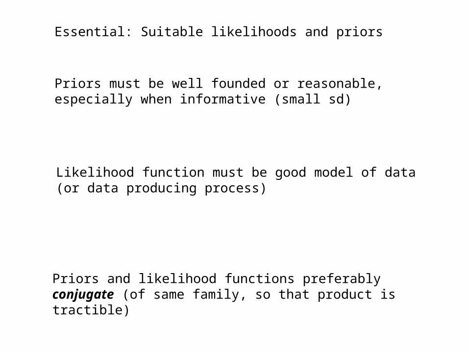
Essential: Suitable likelihoods and priors
Priors must be well founded or reasonable, especially when informative (small sd)
Likelihood function must be good model of data (or data producing process)
Priors and likelihood functions preferably conjugate (of same family, so that product is tractible)
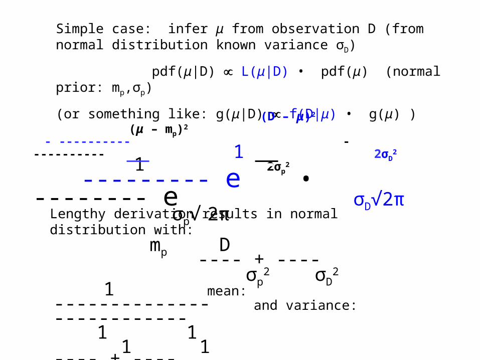
Simple case: infer μ from observation D (from normal distribution known variance σD)
pdf(μ|D) L(μ|D) • pdf(μ) (normal prior: mp,σp)
(or something like: g(μ|D) f(D|μ) • g(μ) )
Lengthy derivation results in normal distribution with:
(D – μ)2 (μ – mp)2
- ---------- - ---------- 1 2σD
2 1 2σp2
--------- e • -------- e σD√2π σp√ 2π
mp D ---- + ----σp
2 σD2 1
mean: -------------- and variance: ------------ 1 1 1 1
---- + ---- ---- + ---- σp
2 σD2 σp
2 σD
2
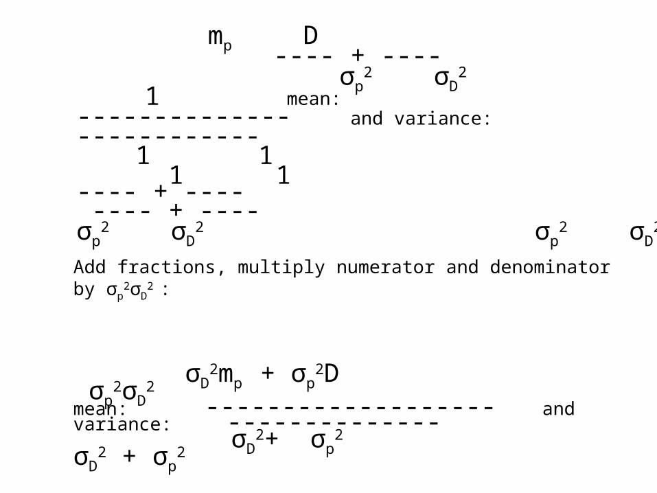
mp D ---- + ----σp
2 σD2 1
mean: -------------- and variance: ------------ 1 1 1 1
---- + ---- ---- + ---- σp
2 σD2 σp
2 σD
2
Add fractions, multiply numerator and denominator by σp2σD
2 :
σD2mp + σp
2D σp2σD
2 mean: ------------------- and variance: --------------
σD2+ σp
2 σD2 + σp
2
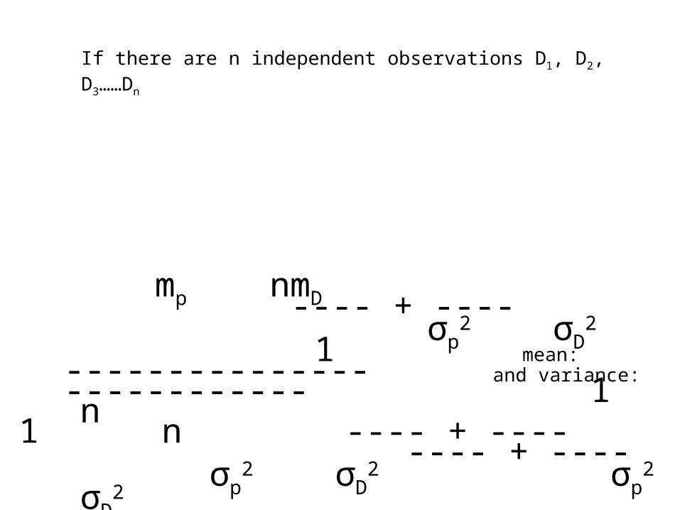
If there are n independent observations D1, D2, D3……Dn
mp nmD ---- + ----σp
2 σD2 1
mean: --------------- and variance: ------------ 1 n 1 n ---- + ---- ---- + ---- σp
2 σD2 σp
2 σD2
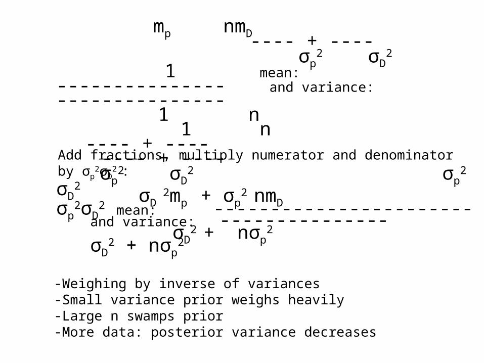
Add fractions, multiply numerator and denominator by σp2σD
2 :
σD 2mp + σp
2 nmD σp
2σD2
mean: ----------------------- and variance: --------------- σD
2 + nσp
2 σD2 + nσp
2
mp nmD ---- + ----σp
2 σD2 1
mean: --------------- and variance: --------------- 1 n 1 n
---- + ---- ---- + ---- σp
2 σD2 σp
2 σD
2
-Weighing by inverse of variances -Small variance prior weighs heavily-Large n swamps prior -More data: posterior variance decreases
Example ofBayesian statistics at UU(approach Hoijtink c.s.)
Bayesian “AN(C)OVA”In stead of: “is there a significant difference between groups – and if so which? ”
“how much support from data to specific informative models?”
Global description! For more information see:
Klugkist,I., Laudy,O. & Hoijtink, H. (2005). Inequality constrained analysis of variance: A Bayesian approach. Psychological Methods, 10, 477-493.
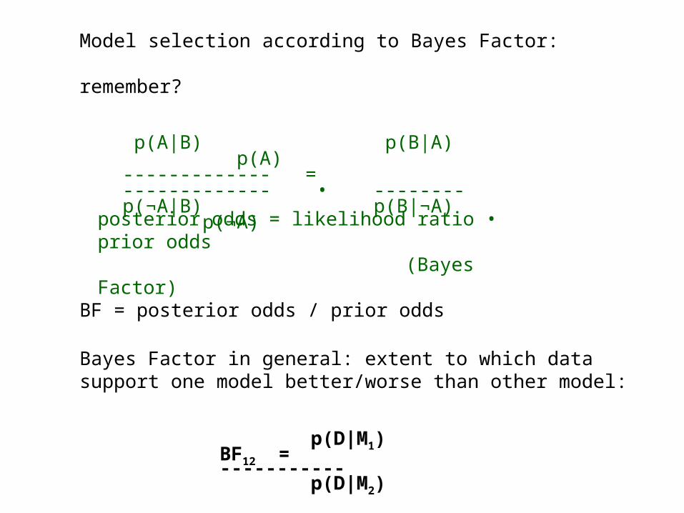
p(A|B) p(B|A) p(A) ------------- = ------------- • -------- p(¬A|B) p(B|¬A) p(¬A)
posterior odds = likelihood ratio • prior odds (Bayes Factor)
Model selection according to Bayes Factor:
remember?
BF = posterior odds / prior odds
Bayes Factor in general: extent to which data support one model better/worse than other model:
p(D|M1)BF12 = -----------
p(D|M2)
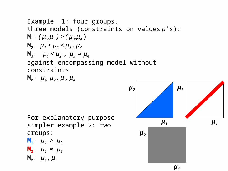
Example 1: four groups.three models (constraints on values μ’s): M1: ( μ1,μ2 ) > ( μ3,μ4 )
M2: μ1 < μ2 < μ3 , μ4 M3: μ1 < μ2 , μ3 ≈ μ4
against encompassing model without constraints:M0: μ1, μ2 , μ3, μ4
For explanatory purpose simpler example 2: two groups:M1: μ1 > μ2
M2: μ1 ≈ μ2
M0: μ1 , μ2
μ2
μ1
μ2
μ1
μ2
μ1

Compute posterior (≈likelihood) for encompassing model (M0)-given data
specify diffuse prior for M0
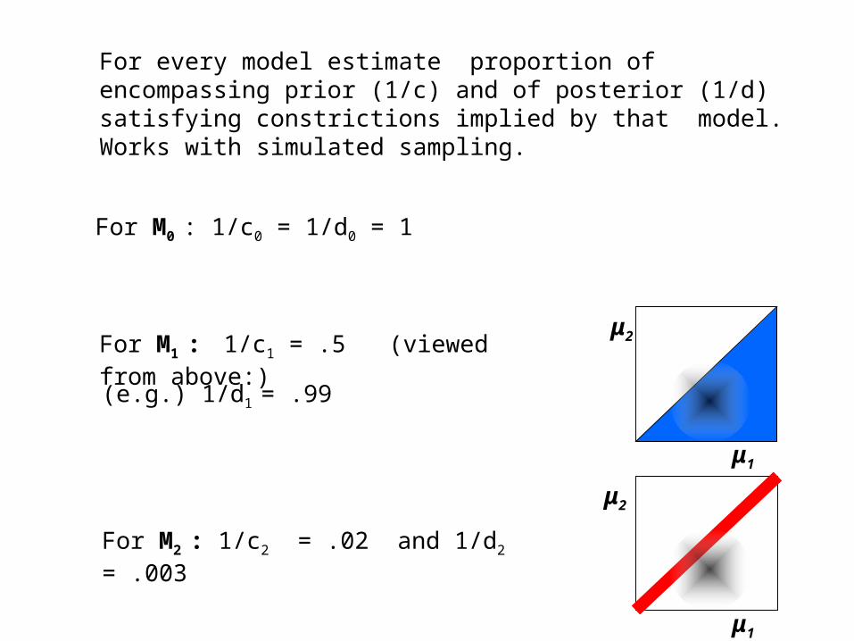
For every model estimate proportion of encompassing prior (1/c) and of posterior (1/d) satisfying constrictions implied by that model. Works with simulated sampling.
For M0 : 1/c0 = 1/d0 = 1
For M1 : 1/c1 = .5 (viewed from above:)μ2
μ1
(e.g.) 1/d1 = .99
μ2
μ1
For M2 : 1/c2 = .02 and 1/d2 = .003
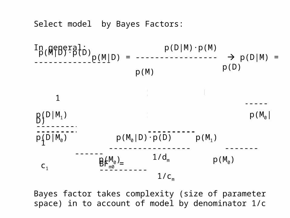
Select model by Bayes Factors:
In general: p(D|M)∙p(M) p(M|D)∙p(D)p(M|D) = ----------------- p(D|M) = ----------------
p(D) p(M)
p(M1|D)∙p(D) p(M1|D) 1 ------------------ ---------- ------
p(D|M1) p(M1) p(M0|D) d1----------- = ------------------------ = ----------------- = -------------p(D|M0) p(M0|D)∙p(D) p(M1) 1
----------------- ------- ------ p(M0) p(M0) c1
1/dmBFm0 = ----------
1/cm
Bayes factor takes complexity (size of parameter space) in to account of model by denominator 1/c
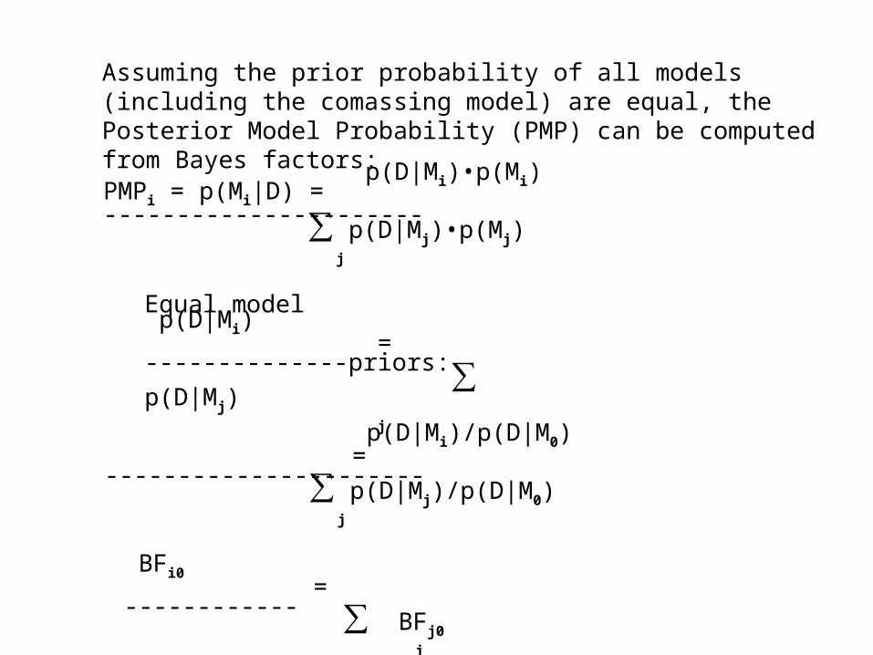
Assuming the prior probability of all models (including the comassing model) are equal, the Posterior Model Probability (PMP) can be computed from Bayes factors:
p(D|Mi)•p(Mi)PMPi = p(Mi|D) = ---------------------- ∑ p(D|Mj)•p(Mj) j
Equal model p(D|Mi) = --------------
priors: ∑ p(D|Mj) j
p(D|Mi)/p(D|M0) = ----------------------
∑ p(D|Mj)/p(D|M0) j
BFi0 = ------------
∑ BFj0 j
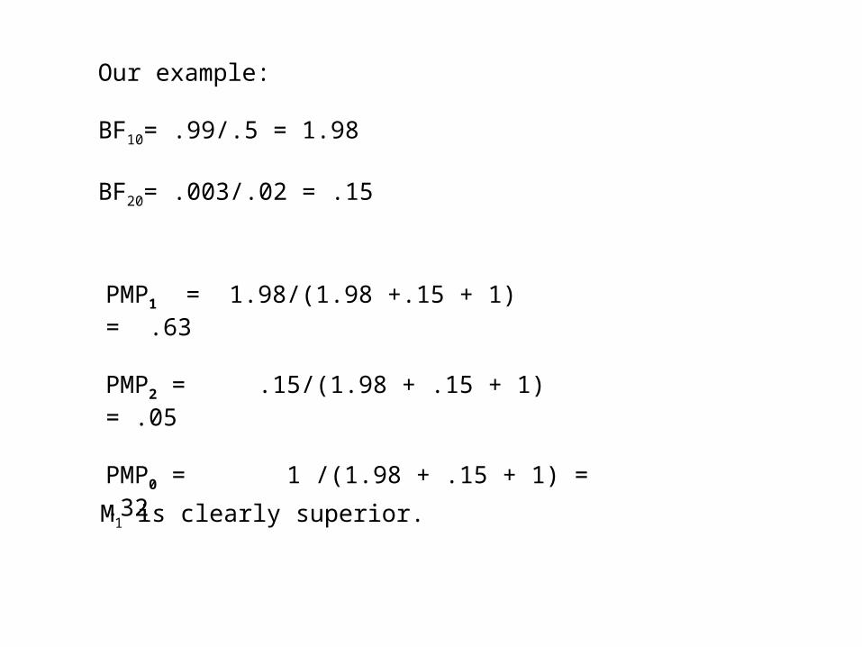
Our example:
BF10= .99/.5 = 1.98
BF20= .003/.02 = .15
M1 is clearly superior.
PMP1 = 1.98/(1.98 +.15 + 1) = .63
PMP2 = .15/(1.98 + .15 + 1) = .05
PMP0 = 1 /(1.98 + .15 + 1) = .32
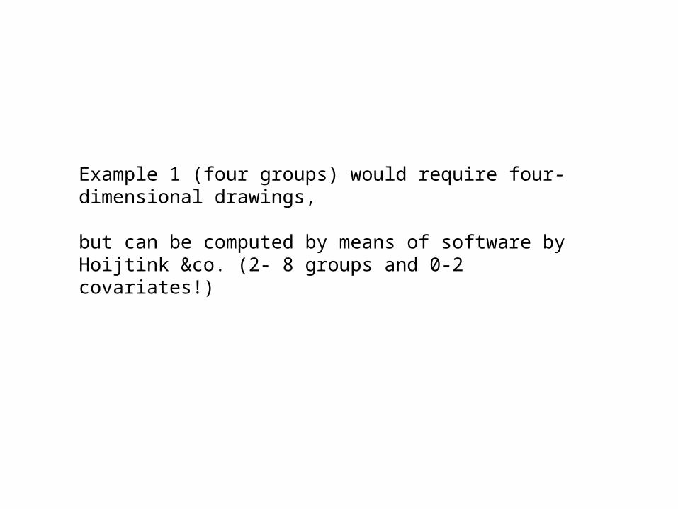
Example 1 (four groups) would require four-dimensional drawings,
but can be computed by means of software by Hoijtink &co. (2- 8 groups and 0-2 covariates!)


![Decision making. Blaise Pascal 1623 - 1662 Probability in games of chance How much should I bet on ’20’? E[gain] = Σgain(x) Pr(x)](https://static.fdocument.org/doc/165x107/56649d565503460f94a34f31/decision-making-blaise-pascal-1623-1662-probability-in-games-of-chance.jpg)