Bayesian Inference for Normal Mean - University of Torontonosedal/sta313/sta313-normal-mean.pdf ·...

Bayesian Inference for Normal Mean

Al Nosedal.University of Toronto.

November 18, 2015

Al Nosedal. University of Toronto. Bayesian Inference for Normal Mean

Likelihood of Single Observation

The conditional observation distribution of y |µ is Normal withmean µ and variance σ2, which is known. Its density is

f (y |µ) =1√2πσ

exp

(− 1

2σ2(y − µ)2

).


Likelihood of Single Observation

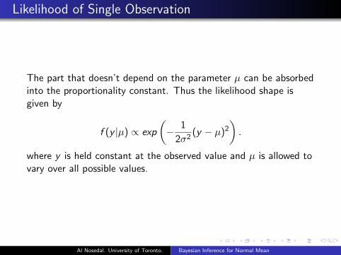
The part that doesn’t depend on the parameter µ can be absorbedinto the proportionality constant. Thus the likelihood shape isgiven by

f (y |µ) ∝ exp

(− 1

2σ2(y − µ)2

).

where y is held constant at the observed value and µ is allowed tovary over all possible values.


Likelihood for a Random Sample of Normal Observations

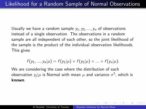
Usually we have a random sample y1, y2, ..., yn of observationsinstead of a single observation. The observations in a randomsample are all independent of each other, so the joint likelihood ofthe sample is the product of the individual observation likelihoods.This gives

f (y1, ..., yn|µ) = f (y1|µ)× f (y2|µ)× ...× f (yn|µ).

We are considering the case where the distribution of eachobservation yj |µ is Normal with mean µ and variance σ2, which isknown.


Finding the posterior probabilities analyzing the sample allat once

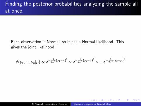
Each observation is Normal, so it has a Normal likelihood. Thisgives the joint likelihood

f (y1, ..., yn|µ) ∝ e−1

2σ2 (y1−µ)2

× e−1

2σ2 (y2−µ)2

× ...e−1

2σ2 (yn−µ)2


Finding the posterior probabilities analyzing the sample allat once

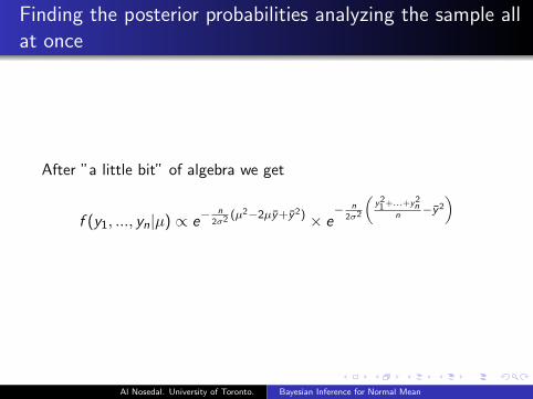
After ”a little bit” of algebra we get

f (y1, ..., yn|µ) ∝ e−n

2σ2 (µ2−2µy+y2) × e− n

2σ2

(y21 +...+y2

nn

−y2

)


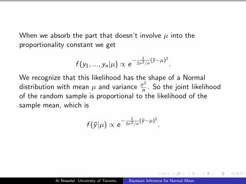
When we absorb the part that doesn’t involve µ into theproportionality constant we get

f (y1, ..., yn|µ) ∝ e− 1

2σ2/n(y−µ)2

.

We recognize that this likelihood has the shape of a Normaldistribution with mean µ and variance σ2

n . So the joint likelihoodof the random sample is proportional to the likelihood of thesample mean, which is

f (y |µ) ∝ e− 1

2σ2/n(y−µ)2

.


Flat Prior Density for µ

The flat prior gives each possible value of µ equal weight. It doesnot favor any value over any other value, g(µ) = 1. The flat prioris not really a proper prior distribution since −∞ < µ <∞, so itcan’t integrate to 1. Nevertheless, this improper prior works outall right. Even though the prior is improper, the posterior willintegrate to 1, so it is proper.


A single Normal observation y

Let y be a Normally distributed observation with mean µ andknown variance σ2. The likelihood

f (y |µ) ∝ e−1

2σ2 (y−µ)2

,

if we ignore the constant of proportionality.


A single Normal observation y (cont.)

Since the prior always equals 1, the posterior is proportional tothis. Rewrite it as

g(µ|y) ∝ e−1

2σ2 (y−µ)2

.

We recognize from this shape that the posterior is a Normaldistribution with mean y and variance σ2.


Normal Prior Density for µ

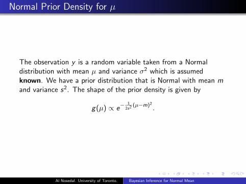
The observation y is a random variable taken from a Normaldistribution with mean µ and variance σ2 which is assumedknown. We have a prior distribution that is Normal with mean mand variance s2. The shape of the prior density is given by

g(µ) ∝ e−1

2s2 (µ−m)2

.


Posterior

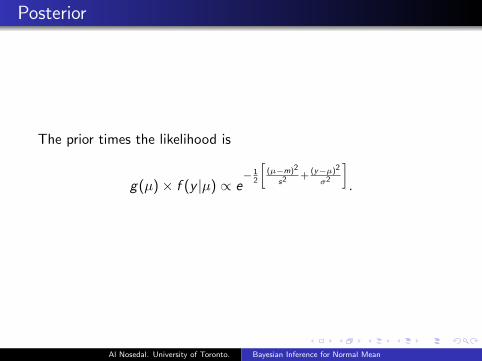
The prior times the likelihood is

g(µ)× f (y |µ) ∝ e− 1

2

[(µ−m)2

s2 + (y−µ)2

σ2

].


Posterior (cont.)

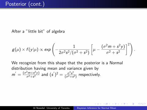
After a ”little bit” of algebra

g(µ)× f (y |µ) ∝ exp

(− 1

2σ2s2/(σ2 + s2)

[µ− (σ2m + s2y)

σ2 + s2

]2).

We recognize from this shape that the posterior is a Normaldistribution having mean and variance given by

m′

= (σ2m+s2y)σ2+s2 and (s

′)2 = σ2s2

(σ2+s2)respectively.


Simple updating rule for Normal family

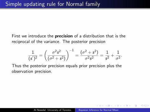
First we introduce the precision of a distribution that is thereciprocal of the variance. The posterior precision

1

(s ′)2=

(σ2s2

(σ2 + s2)

)−1

=(σ2 + s2)

σ2s2=

1

s2+

1

σ2.

Thus the posterior precision equals prior precision plus theobservation precision.


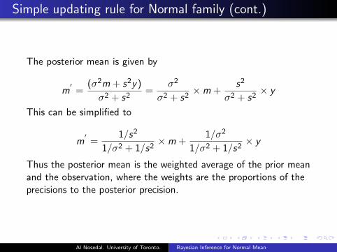
Simple updating rule for Normal family (cont.)

The posterior mean is given by

m′

=(σ2m + s2y)

σ2 + s2=

σ2

σ2 + s2×m +

s2

σ2 + s2× y

This can be simplified to

m′

=1/s2

1/σ2 + 1/s2×m +

1/σ2

1/σ2 + 1/s2× y

Thus the posterior mean is the weighted average of the prior meanand the observation, where the weights are the proportions of theprecisions to the posterior precision.


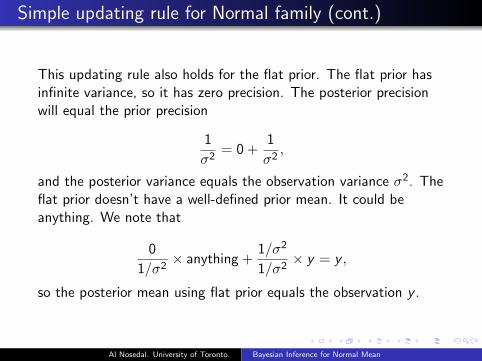
Simple updating rule for Normal family (cont.)

This updating rule also holds for the flat prior. The flat prior hasinfinite variance, so it has zero precision. The posterior precisionwill equal the prior precision

1

σ2= 0 +

1

σ2,

and the posterior variance equals the observation variance σ2. Theflat prior doesn’t have a well-defined prior mean. It could beanything. We note that

0

1/σ2× anything +

1/σ2

1/σ2× y = y ,

so the posterior mean using flat prior equals the observation y .


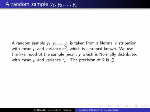
A random sample y1, y2, ..., yn

A random sample y1, y2, ..., yn is taken from a Normal distributionwith mean µ and variance σ2, which is assumed known. We usethe likelihood of the sample mean, y which is Normally distributedwith mean µ and variance σ2

n . The precision of y is nσ2 .


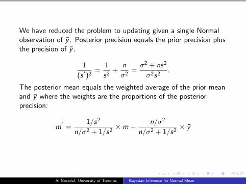
We have reduced the problem to updating given a single Normalobservation of y . Posterior precision equals the prior precision plusthe precision of y .

1

(s ′)2=

1

s2+

n

σ2=σ2 + ns2

σ2s2.

The posterior mean equals the weighted average of the prior meanand y where the weights are the proportions of the posteriorprecision:

m′

=1/s2

n/σ2 + 1/s2×m +

n/σ2

n/σ2 + 1/s2× y


Equivalent Prior Sample Size

A useful check on your prior is to consider the ”equivalent samplesize”. Set your prior variance s2 = σ2

neqand solve for neq. This

relates your prior precision to the precision from a sample. Yourbelief is of equal importance to a sample of size neq.


Specifying Prior Parameters

We already saw that there were many strategies for picking theparameter values for a beta prior to go with a binomial likelihood.Similar approaches work for specifying the parameters of a normalprior for a normal mean. Often we will have some degree ofknowledge about where the normal population is centered, sochoosing the mean of the prior distribution for µ usually is lessdifficult than picking the prior variance (or precision). Workablestrategies include:

Graph normal densities with different variances until you findone that matches your prior information.

Identify an interval which you believe has 95% probability oftrapping the true value of µ, and find the normal density thatproduces it.

Quantify your degree of certainty about the value of µ interms of equivalent prior sample size.


Example

Arnie and Barb are going to estimate the mean length ofone-year-old rainbow trout in a stream. Previous studies in otherstreams have shown the length of yearling rainbow trout to beNormally distributed with known standard deviation of 2 cm. Arniedecides his prior mean is 30 cm. He decides that he doesn’t believeit is possible for a yearling rainbow to be less than 18 cm or greaterthan 42 cm. Thus his prior standard deviation is 4 cm. Thus hewill use a Normal(30, 4) prior. Barb doesn’t know anything abouttrout, so she decides to use the ”flat” prior.


Example (cont.)

They take a random sample of 12 yearling trout from the streamand find the sample mean y = 32 cm. Arnie and Barb find theirposterior distributions using the simple updating rules for theNormal conjugate family.


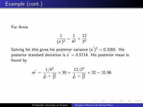
Example (cont.)

For Arnie

1

(s ′)2=

1

42+

12

22

Solving for this gives his posterior variance (s′)2 = 0.3265. His

posterior standard deviation is s′

= 0.5714. His posterior mean isfound by

m′

=1/42

142 + 12

22

× 30 +12/22

142 + 12

22

× 32 = 31.96


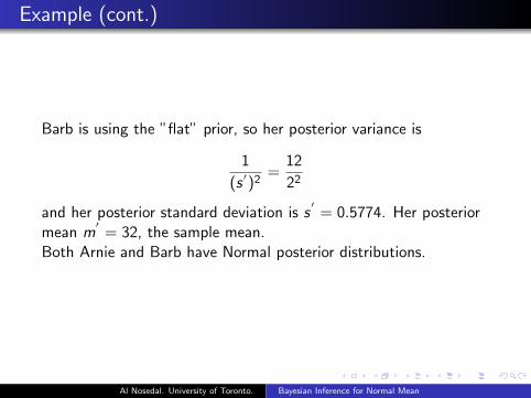
Example (cont.)

Barb is using the ”flat” prior, so her posterior variance is

1

(s ′)2=

12

22

and her posterior standard deviation is s′

= 0.5774. Her posteriormean m

′= 32, the sample mean.

Both Arnie and Barb have Normal posterior distributions.


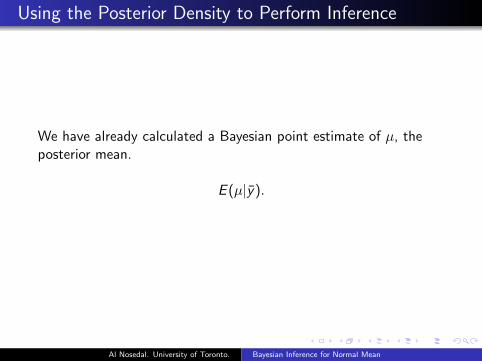
Using the Posterior Density to Perform Inference

We have already calculated a Bayesian point estimate of µ, theposterior mean.

E (µ|y).


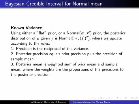
Bayesian Credible Interval for Normal mean

Known VarianceUsing either a ”flat” prior, or a Normal(m, s2) prior, the posteriordistribution of µ given y is Normal(m

′, (s′)2), where we update

according to the rules:1. Precision is the reciprocal of the variance.2. Posterior precision equals prior precision plus the precision ofsample mean.3. Posterior mean is weighted sum of prior mean and samplemean, where the weights are the proportions of the precisions tothe posterior precision.



Our (1− α)× 100% Bayesian Credible Interval for µ is

m′ ± zα/2 × s

′,

where the z-value is found in the standard Normal table. Since theposterior distribution is Normal and thus symmetric, the credibleinterval found is the shortest, as well as having equal tailprobabilities.



Unknown VarianceIf we don’t know the variance, we don’t know the precision, so wecan’t use the updating rules directly. The obvious thing to do is tocalculate the sample variance

σ2 =1

n − 1

n∑i=1

(yi − y)2

from the data. Then we use our equations to find (s′)2 and m

′

where we use the sample variance σ2 in place of the unknownvariance σ2.


Bayesian Credible Interval for Normal mean (cont.)

Unknown VarianceThere is extra uncertainty here, the uncertainty in estimating σ2.We should widen the credible interval to account for this addeduncertainty. We do this by taking the values from the Student’s ttable instead of the Standard Normal table. The correct Bayesiancredible interval is

m′ ± tα/2 × s

′.

The t value is taken from the row labelled df = n − 1 (degrees offreedom equals number of observations minus 1)∗.


∗ The resulting Bayesian credible interval is exactly the same onethat we would find if we did the full Bayesian analysis with σ2 as anuisance parameter, using the joint prior distribution for µ and σ2

made up of the same prior for µ|σ2 that we used before (”flat” orNormal(m, s2)) times the prior for σ2 given by g(σ2) ∝ (σ2)−1.We would find the joint posterior by Bayes’ Theorem. We wouldfind the marginal posterior distribution of µ by marginalizing outσ2. We would get the same Bayesian credible interval usingStudent’s t critical values.


Example

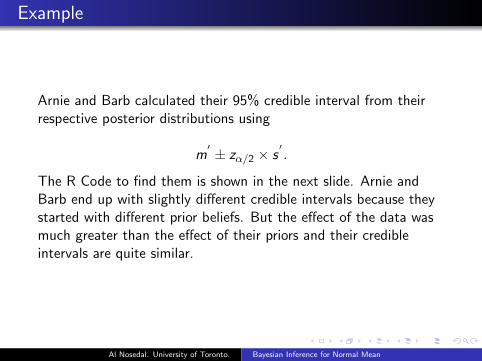
Arnie and Barb calculated their 95% credible interval from theirrespective posterior distributions using

m′ ± zα/2 × s

′.

The R Code to find them is shown in the next slide. Arnie andBarb end up with slightly different credible intervals because theystarted with different prior beliefs. But the effect of the data wasmuch greater than the effect of their priors and their credibleintervals are quite similar.


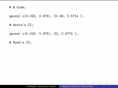
# R Code;

qnorm( c(0.025, 0.975), 31.96, 0.5714 );

# Arnie’s CI;

qnorm( c(0.025, 0.975), 32, 0.5774 );

# Barb’s CI;


Predictive Density for next observation

Let yn+1 be the next random variable drawn after the randomsample y1, y2, ..., yn. The predictive density of yn+1|y1, y2, ..., yn isthe conditional density

f (yn+1|y1, y2, ..., yn).



The conditional distribution we want is found by integrating µ outof the joint posterior distribution.

f (yn+1|y1, y2, ..., yn) =

∫f (yn+1|µ)× g(µ|y1, y2, ..., yn)dµ.



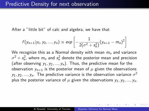
After a ”little bit” of calc and algebra, we have that

f (yn+1|y1, y2, ..., yn) ∝ exp

[− 1

2(σ2 + s2n)

(yn+1 −mn)2

]We recognize this as a Normal density with mean mn and varianceσ2 + s2

n , where mn and s2n denote the posterior mean and precision

(after observing y1, y2, ..., yn). Thus, the predictive mean for theobservation yn+1 is the posterior mean of µ given the observationsy1, y2, ..., yn. The predictive variance is the observation variance σ2

plus the posterior variance of µ given the observations y1, y2, ..., yn.


Bayesian One-sided Hypothesis Test about µ

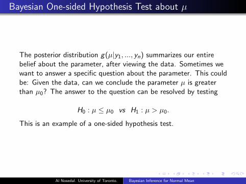
The posterior distribution g(µ|y1, ..., yn) summarizes our entirebelief about the parameter, after viewing the data. Sometimes wewant to answer a specific question about the parameter. This couldbe: Given the data, can we conclude the parameter µ is greaterthan µ0? The answer to the question can be resolved by testing

H0 : µ ≤ µ0 vs H1 : µ > µ0.

This is an example of a one-sided hypothesis test.


Bayesian One-sided Hypothesis Test about µ

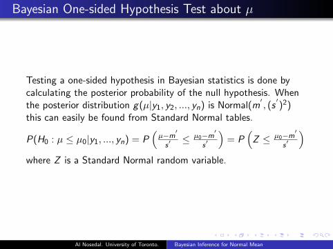
Testing a one-sided hypothesis in Bayesian statistics is done bycalculating the posterior probability of the null hypothesis. Whenthe posterior distribution g(µ|y1, y2, ..., yn) is Normal(m

′, (s′)2)

this can easily be found from Standard Normal tables.

P(H0 : µ ≤ µ0|y1, ..., yn) = P(µ−m

′

s′≤ µ0−m

′

s′

)= P

(Z ≤ µ0−m

′

s′

)where Z is a Standard Normal random variable.


Example

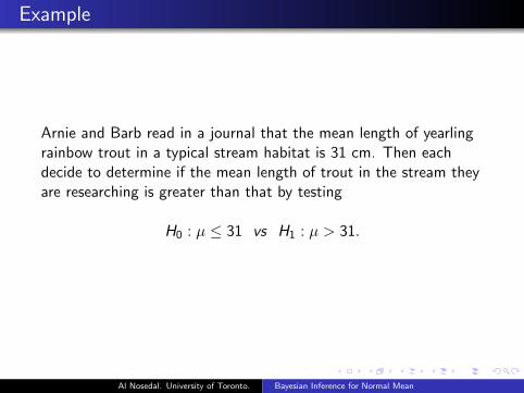
Arnie and Barb read in a journal that the mean length of yearlingrainbow trout in a typical stream habitat is 31 cm. Then eachdecide to determine if the mean length of trout in the stream theyare researching is greater than that by testing

H0 : µ ≤ 31 vs H1 : µ > 31.


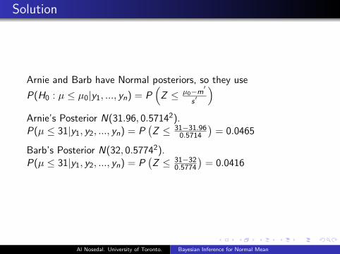
Solution

Arnie and Barb have Normal posteriors, so they use

P(H0 : µ ≤ µ0|y1, ..., yn) = P(Z ≤ µ0−m

′

s′

)Arnie’s Posterior N(31.96, 0.57142).P(µ ≤ 31|y1, y2, ..., yn) = P

(Z ≤ 31−31.96

0.5714

)= 0.0465

Barb’s Posterior N(32, 0.57742).P(µ ≤ 31|y1, y2, ..., yn) = P

(Z ≤ 31−32

0.5774

)= 0.0416


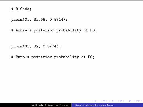
# R Code;

pnorm(31, 31.96, 0.5714);

# Arnie’s posterior probability of H0;

pnorm(31, 32, 0.5774);

# Barb’s posterior probability of H0;


Bayesian Two-sided Hypothesis Test about µ

Sometimes the question we want to have answered is: Is the meanfor the new population µ, the same as the mean for the standardpopulation which we know equals µ0? A two-sided hypothesis testattempts to answer this question. We set this up as

H0 : µ = µ0 vs Ha : µ 6= µ0.


Bayesian Two-Sided Hypothesis Test about µ

If we wish to test the two-sided hypothesis

H0 : µ = µ0 vs Ha : µ 6= µ0.

in a Bayesian manner, and we have a continuous prior, we can’tcalculate the posterior probability of the null hypothesis as we didfor the one-sided hypothesis. We know that the probability of anyspecific value of a continuous random variable always equals 0.The posterior probability of the null hypothesis H0 : µ = µ0 willequal zero.


Bayesian Two-Sided Hypothesis Test about µ

Instead, we calculate a (1−α)× 100% credible interval for µ usingour posterior distribution. If µ0 lies inside the credible interval, weconclude that µ0 still has credibility as a possible value. In thatcase we will not reject the null hypothesis H0 : µ = µ0.


Bayesian Inference for Normal Mean - University of Torontonosedal/sta313/sta313-normal-mean.pdf ·...

Documents

Transcript of Bayesian Inference for Normal Mean - University of Torontonosedal/sta313/sta313-normal-mean.pdf ·...