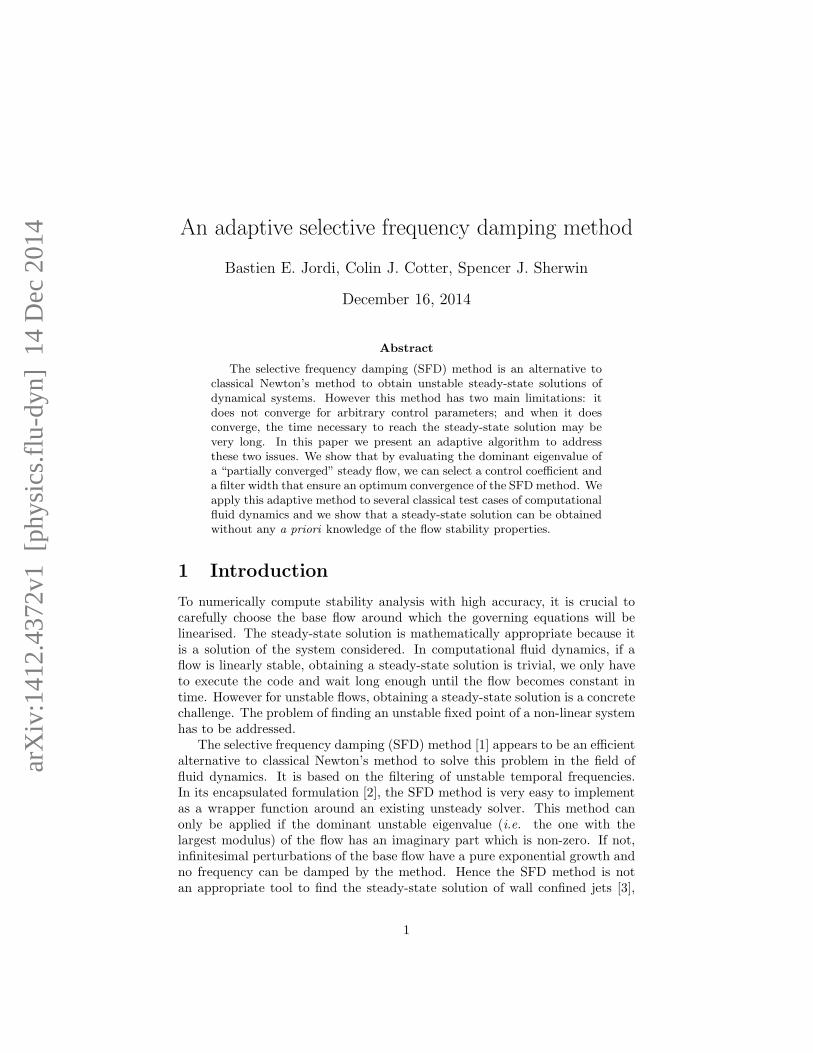
arX

iv:1

412.

4372

v1 [

phys

ics.

flu-

dyn]

14

Dec

201

4 An adaptive selective frequency damping method

Bastien E. Jordi, Colin J. Cotter, Spencer J. Sherwin

December 16, 2014

Abstract

The selective frequency damping (SFD) method is an alternative toclassical Newton’s method to obtain unstable steady-state solutions ofdynamical systems. However this method has two main limitations: itdoes not converge for arbitrary control parameters; and when it doesconverge, the time necessary to reach the steady-state solution may bevery long. In this paper we present an adaptive algorithm to addressthese two issues. We show that by evaluating the dominant eigenvalue ofa “partially converged” steady flow, we can select a control coefficient anda filter width that ensure an optimum convergence of the SFD method. Weapply this adaptive method to several classical test cases of computationalfluid dynamics and we show that a steady-state solution can be obtainedwithout any a priori knowledge of the flow stability properties.

1 Introduction

To numerically compute stability analysis with high accuracy, it is crucial tocarefully choose the base flow around which the governing equations will belinearised. The steady-state solution is mathematically appropriate because itis a solution of the system considered. In computational fluid dynamics, if aflow is linearly stable, obtaining a steady-state solution is trivial, we only haveto execute the code and wait long enough until the flow becomes constant intime. However for unstable flows, obtaining a steady-state solution is a concretechallenge. The problem of finding an unstable fixed point of a non-linear systemhas to be addressed.

The selective frequency damping (SFD) method [1] appears to be an efficientalternative to classical Newton’s method to solve this problem in the field offluid dynamics. It is based on the filtering of unstable temporal frequencies.In its encapsulated formulation [2], the SFD method is very easy to implementas a wrapper function around an existing unsteady solver. This method canonly be applied if the dominant unstable eigenvalue (i.e. the one with thelargest modulus) of the flow has an imaginary part which is non-zero. If not,infinitesimal perturbations of the base flow have a pure exponential growth andno frequency can be damped by the method. Hence the SFD method is notan appropriate tool to find the steady-state solution of wall confined jets [3],

1

for example. However the SFD method can be used to obtain the steady-statesolutions of flows with oscillatory growth of the instabilities.

The convergence of the SFD method is governed by two parameters, whichare the control coefficient χ and the filter width ∆. For arbitrary choice ofthese parameters, the method may not be able to control the evolution of theinstabilities within the flow. Hence the method does not always converge. Evenwhen a steady-state solution can be found, convergence may be very slow. Theselection of the parameters χ and ∆ is central for users of the SFD method. Weintend to address this issue in this study.

We present an adaptive procedure that couples the SFD method and a globalstability analysis method. The idea is to approximate the dominant eigenvalueof the flow studied during the execution of the solver implementing the SFDmethod. This approximation is used to tune χ and ∆ by using a simple one-dimensional model. The strength of this procedure is that it does not requireany knowledge of the flow behaviour before executing the code.

In Sec. 2 we summarise the properties of the encapsulated formulation ofthe SFD method. In Sec. 3 we present the main aspects of global stabilityanalysis and recall a modified Arnoldi iteration method [4] that evaluates thedominant eigenvalue of a given base flow. In Sec. 4 we show how optimumparameters of the SFD method can be selected when the dominant eigenvalueof the system studied is known. In Sec. 5 we present an adaptive procedureto automatically select parameters that ensure an optimum convergence of theSFD method. Finally in Sec. 6 we show that this procedure can be successfullyapplied to obtain unstable steady-state solutions of several classical test casesof computational fluid dynamics. This set of test cases aims to validate theadaptive method prior to its application to more challenging flows.

2 Encapsulated SFD method

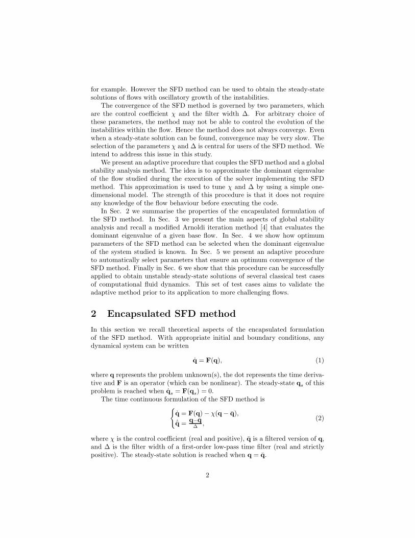
In this section we recall theoretical aspects of the encapsulated formulationof the SFD method. With appropriate initial and boundary conditions, anydynamical system can be written

q = F(q), (1)

where q represents the problem unknown(s), the dot represents the time deriva-tive and F is an operator (which can be nonlinear). The steady-state qs of thisproblem is reached when qs = F(qs) = 0.

The time continuous formulation of the SFD method is{

q = F(q)− χ(q− q),

˙q =q−q∆

,(2)

where χ is the control coefficient (real and positive), q is a filtered version of q,and ∆ is the filter width of a first-order low-pass time filter (real and strictlypositive). The steady-state solution is reached when q = q.

2

For a given space and time discretization of (1), we define Φ as the functionreading qn+1 and qn+1 i.e.

qn+1 = Φ(qn). (3)

To implement the encapsulated formulation of the SFD method, system (2)is divided into two smaller (simpler) subproblems using the framework of first-order splitting methods [5]. The first subproblem is simply (1) and the secondsubproblem is linear and models the influence of the feedback control and thelow-pass time filter (i.e. its expression is identical to (2) without the term F(q)).Hence at step (n+ 1), the solution of the controlled system is given by

(qn+1

qn+1

)

= eL∆t

(Φ(qn)qn

)

, (4)

where ∆t is the time-step used within the solver Φ and, if we note I is theidentity matrix, the linear operator L is such that

L =

(−χI χII/∆ −I/∆

)

. (5)

This method is called encapsulated because the existing unsteady time-stepper Φ does not need to be modified. This solver is simply treated as a“black box” and the method can be implemented as a wrapper function aroundit. The action of this wrapper is only to apply the linear operator eL∆t to theoutput of Φ and to the filtered quantity qn at every time step.

System (4) does not converge towards the steady-state solution of (1) forarbitrary control coefficient χ and filter width ∆. These parameters have tobe carefully chosen to control the evolution of the least stable mode of (1). InSec. 3 we present a method to evaluate this least stable mode. Then in Sec. 4we show how optimum parameters χ and ∆ can be selected once the dominanteigenvalue of (1) is known.

3 Global stability analysis using time-stepping

In this section we present an overview of the main aspects of global stabilityproblems in fluid dynamics. System (1) models any dynamical system, but herewe only focus on the incompressible Navier-Stokes equations

{

∂tu = − (u · ∇)u−∇p+Re−1∇2u,

∇ · u = 0,(6)

where u is the fluid velocity and p is the modified (or kinematic) pressure.Re = u∞L/ν is the Reynolds number where u∞ is the mean velocity, L is thecharacteristic length and ν is the kinematic viscosity. Appropriate initial andboundary conditions must also be defined.

The starting point of linear stability analysis is to define a base flow U whichis a solution of (6). This base flow can be time-dependent (e.g. Floquet stability

3

analysis requires a time-periodic base flow) but in this study, we are interestedin steady base flows. In this section, we assume that a steady-state solution of(6) is known.

Subject to appropriate initial and boundary conditions, the evolution ofinfinitesimal perturbations u′ of the base flow U is governed by the linearisedNavier-Stokes equations

{

∂tu′ = − (U · ∇)u′ − (u′ · ∇)U−∇p′ +Re−1∇2u′,

∇ · u′ = 0.(7)

A linear evolution operator A can be defined from Eq. (7). Hence an initialperturbation u′(0) evolves forward in time such that

u′(t) = A(t)u′(0). (8)

Note that to correctly set up system (8), the inflow boundary conditions ofthe non-linear problem have to be modified to be homogeneous Dirichlet.

We are interested in normal mode solutions of the form u′(x, t)=exp(µjt)uj(x) + c.c., where uj are the eigenmodes and µj are the eigenvalues (both are,in general, complex). We can define the growth rate σj and the frequency fjsuch that µj = σj + ifj. We also define the time TArnoldi as being the length ofan Arnoldi iteration. TArnoldi has to be large enough to allow the perturbationto evolve because large times increase the spectral gap of A(TArnoldi), whichincreases the convergence rate of the method. For a given time TArnoldi, weobtain the eigenvalue problem

A(TArnoldi)uj = λjuj , with λj = exp(µjTArnoldi). (9)

Linear stability (or instability) of the base flow U is determined by thedominant eigenvalue of A(TArnoldi) (i.e. the one of largest modulus). If thereexists at least one λj such that |λj | > 1, then infinitesimal perturbations ofthe base flow exponentially grow in time. Hence U is said to be asymptoticallylinearly unstable. In opposition, if all the eigenvalues verify |λj | < 1, theninfinitesimal perturbations decay in time and the base flow is linearly stable.Most of the time |λj | = 1 indicates a bifurcation point. Note that instead ofevaluating the modulus of the eigenvalues λj , one can also look at the sign of thecorresponding growth rate σj . A negative growth rate corresponds to a linearlystable base flow and a positive growth rate, to an linearly unstable one.

To compute the eigenvalues of A(TArnoldi), the “time-stepper” approach [6, 4]is used. The idea is to perform stability analysis by adapting an existing Navier-Stokes code that solves (6). Note that in Sec. 2 a comparable strategy was used,where the encapsulated SFD method was presented as being easy to implementas a wrapper around an existing unsteady solver.

Dominant eigenvalues are obtained using the modified Arnoldi iterationmethod introduced by Barkley et al [4]. The mechanism of this algorithm isthat the operator A(TArnoldi) is applied several times to a random initial vectoru0 (which is non-zero). This generates a Krylov subspace and then an upper

4

Hessenberg matrix H. The dominant eigenvalue of H converges towards thedominant eigenvalue of A(TArnoldi) in a relatively limited number of iterations.The computational cost and memory requirements of this algorithm are low.The most demanding part is to compute A(TArnoldi) every Arnoldi iteration.

This algorithm has been recently implemented into the Nektar++ spec-tral/hp element framework [7]. Rocco [8] showed that the results agree verywell with ARPACK (ARnoldi PACKage [9]), the differences between the domi-nant eigenvalues obtained with the two methods were found to be smaller that10−5.

Note that, when an adjoint linearised system is implemented, this algorithmcan be adapted to compute transient growth analysis and evaluate the influenceof non-normal modes.

4 Evaluation of optimum parameters

Global stability analysis aims to determine if the largest eigenvalue of the linearoperator A(TArnoldi) has a modulus larger than one or not. When the SFDmethod is applied to a system, it aims to control the evolution of the leaststable eigenvalue of this system. Hence determining if the SFD method cancontrol a dynamical system may be narrowed down to: can the SFD methodcontrol the evolution of the dominant instability of this system?

At this stage, we assume the dominant eigenvalue (denoted λD) of the un-stable dynamical system studied is known. We introduce the one-dimensionalmodel

un+1 = λDun. (10)

For a given control coefficient χ and filter width ∆, if the SFD method isable to force (10) to evolve towards its steady-state (which is u = u = 0), itmeans that it is able to control the instabilities related to λD. Then the sameparameters can be used in the SFD method applied to an unstable fluid systemwhich has λD for dominant eigenvalue. The encapsulated formulation of theSFD method is applied to (10), is such that

(un+1

un+1

)

= eL1D

(λDun

un

)

= eL1D

(λD 00 1

)

︸ ︷︷ ︸

M

(un

un

)

, (11)

where L1D is similar to (5), with I replaced by 1, and M is the iteration matrixtransforming (un, un) into (un+1, un+1). M depends on λD, χ and ∆.

The convergence of (11) is only governed by the two eigenvalues ofM. If theyboth have a modulus strictly smaller than one, then system (11) is stable andconverges towards its steady-state solution. Otherwise, the system is unstableand the steady-state can not be reached.

As M is a 2 by 2 matrix, evaluating the modulus of its eigenvalues is simple.For a fixed λD, we can manually select a control coefficient χ and a filter width ∆that ensure both eigenvalues ofM to be smaller than one. Then the instabilities

5

are controlled by the SFD method and convergence of (11) towards its steady-state is guaranteed. However, this convergence may be slow.

The fastest convergence of (11) is achieved when the modulus of the dom-inant eigenvalue of M is minimum. As we can evaluate the eigenvalues of Mfor every χ > 0 and every ∆ > 0 (for a fixed λD), a basic line search algorithmcan be implemented to obtain the optimum parameters χopt and ∆opt that givethe minimum of the modulus of the dominant eigenvalue of M. Then theseparameters can be used in the SFD method applied to a flow which has λD fordominant eigenvalue.

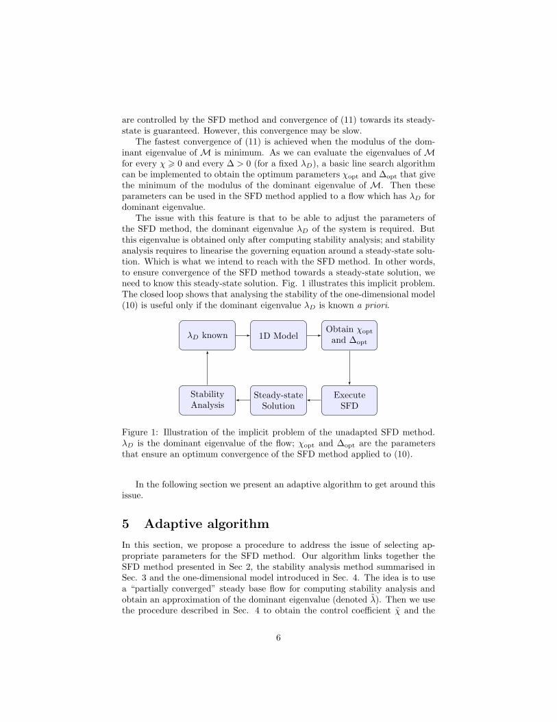
The issue with this feature is that to be able to adjust the parameters ofthe SFD method, the dominant eigenvalue λD of the system is required. Butthis eigenvalue is obtained only after computing stability analysis; and stabilityanalysis requires to linearise the governing equation around a steady-state solu-tion. Which is what we intend to reach with the SFD method. In other words,to ensure convergence of the SFD method towards a steady-state solution, weneed to know this steady-state solution. Fig. 1 illustrates this implicit problem.The closed loop shows that analysing the stability of the one-dimensional model(10) is useful only if the dominant eigenvalue λD is known a priori.

λD known 1D ModelObtain χopt

and ∆opt

ExecuteSFD

Steady-stateSolution

StabilityAnalysis

Figure 1: Illustration of the implicit problem of the unadapted SFD method.λD is the dominant eigenvalue of the flow; χopt and ∆opt are the parametersthat ensure an optimum convergence of the SFD method applied to (10).

In the following section we present an adaptive algorithm to get around thisissue.

5 Adaptive algorithm

In this section, we propose a procedure to address the issue of selecting ap-propriate parameters for the SFD method. Our algorithm links together theSFD method presented in Sec 2, the stability analysis method summarised inSec. 3 and the one-dimensional model introduced in Sec. 4. The idea is to usea “partially converged” steady base flow for computing stability analysis andobtain an approximation of the dominant eigenvalue (denoted λ). Then we usethe procedure described in Sec. 4 to obtain the control coefficient χ and the

6

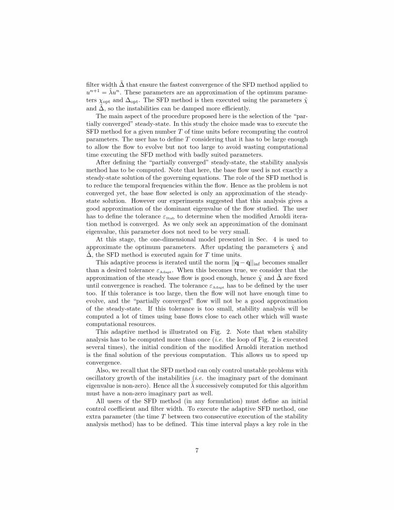
filter width ∆ that ensure the fastest convergence of the SFD method applied toun+1 = λun. These parameters are an approximation of the optimum parame-ters χopt and ∆opt. The SFD method is then executed using the parameters χ

and ∆, so the instabilities can be damped more efficiently.The main aspect of the procedure proposed here is the selection of the “par-

tially converged” steady-state. In this study the choice made was to execute theSFD method for a given number T of time units before recomputing the controlparameters. The user has to define T considering that it has to be large enoughto allow the flow to evolve but not too large to avoid wasting computationaltime executing the SFD method with badly suited parameters.

After defining the “partially converged” steady-state, the stability analysismethod has to be computed. Note that here, the base flow used is not exactly asteady-state solution of the governing equations. The role of the SFD method isto reduce the temporal frequencies within the flow. Hence as the problem is notconverged yet, the base flow selected is only an approximation of the steady-state solution. However our experiments suggested that this analysis gives agood approximation of the dominant eigenvalue of the flow studied. The userhas to define the tolerance εStab to determine when the modified Arnoldi itera-tion method is converged. As we only seek an approximation of the dominanteigenvalue, this parameter does not need to be very small.

At this stage, the one-dimensional model presented in Sec. 4 is used toapproximate the optimum parameters. After updating the parameters χ and∆, the SFD method is executed again for T time units.

This adaptive process is iterated until the norm ||q− q||inf becomes smallerthan a desired tolerance εAdapt. When this becomes true, we consider that theapproximation of the steady base flow is good enough, hence χ and ∆ are fixeduntil convergence is reached. The tolerance εAdapt has to be defined by the usertoo. If this tolerance is too large, then the flow will not have enough time toevolve, and the “partially converged” flow will not be a good approximationof the steady-state. If this tolerance is too small, stability analysis will becomputed a lot of times using base flows close to each other which will wastecomputational resources.

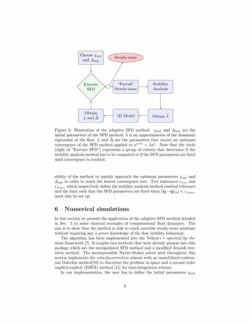
This adaptive method is illustrated on Fig. 2. Note that when stabilityanalysis has to be computed more than once (i.e. the loop of Fig. 2 is executedseveral times), the initial condition of the modified Arnoldi iteration methodis the final solution of the previous computation. This allows us to speed upconvergence.

Also, we recall that the SFD method can only control unstable problems withoscillatory growth of the instabilities (i.e. the imaginary part of the dominanteigenvalue is non-zero). Hence all the λ successively computed for this algorithmmust have a non-zero imaginary part as well.

All users of the SFD method (in any formulation) must define an initialcontrol coefficient and filter width. To execute the adaptive SFD method, oneextra parameter (the time T between two consecutive execution of the stabilityanalysis method) has to be defined. This time interval plays a key role in the

7

Choose χinit

and ∆init

ExecuteSFD

“Partial”Steady-state

Steady-state

StabilityAnalysis

Obtain λ1D ModelObtainχ and ∆

Figure 2: Illustration of the adaptive SFD method. χinit and ∆init are theinitial parameters of the SFD method; λ is an approximation of the dominanteigenvalue of the flow; χ and ∆ are the parameters that ensure an optimumconvergence of the SFD method applied to un+1 = λun. Note that the circle(right of “Execute SFD”) represents a group of criteria that determine if thestability analysis method has to be computed or if the SFD parameters are fixeduntil convergence is reached.

ability of the method to quickly approach the optimum parameters χopt and∆opt in order to reach the fastest convergence rate. Two tolerances εStab andεAdapt, which respectively define the stability analysis method residual toleranceand the limit such that the SFD parameters are fixed when ||q− q||inf < εAdapt,must also be set up.

6 Numerical simulations

In this section we present the application of the adaptive SFD method detailedin Sec. 5 to some classical examples of computational fluid dynamics. Theaim is to show that the method is able to reach unstable steady-state solutionswithout requiring any a priori knowledge of the flow stability behaviour.

The algorithm has been implemented into the Nektar++ spectral/hp ele-ment framework [7]. It couples two methods that were already present into thispackage which are the encapsulated SFD method and a modified Arnoldi iter-ation method. The incompressible Navier-Stokes solver used throughout thissection implements the velocity-correction scheme with an unstabilised continu-ous Galerkin method[10] to discretize the problem in space and a second orderimplicit-explicit (IMEX) method [11] for time-integration scheme.

In our implementation, the user has to define the initial parameters χinit

8

and ∆init, the time T for which the SFD method is executed before computingstability analysis, the tolerance εStab of the modified Arnoldi iteration methodand the tolerance εAdapt which determines when we stop adapting the controlcoefficient and the filter width. Throughout this section, we fix εStab = 10−3,εAdapt = 10−2 and we considered the problem to be converged when ||q−q||inf <10−8.

Also, we define the length of one Arnoldi iteration to be equal to one timeunit. Hence if the stability analysis converges in n iterations, the computationaltime will be approximately the same as executing the Navier-Stokes solver forn iterations.

Four two-dimensional simulations are presented in this section. In Sec. 6.1the behaviour of the adaptive SFD method is detailed for the incompressibleflow past a cylinder at Re = 100. Then in Sec. 6.2 we show that this case caneasily be extended to higher Reynolds numbers and present the case Re = 300.In Sec. 6.3, the incompressible flow past an ellipse at Re = 150 is also studied inorder to show that the adaptive SFD method works well on geometries that donot contain axial symmetries. Finally in Sec. 6.4 we consider the incompressibleflow past a rotating cylinder at Re = 100 and a rotation rate α = 5, and showthat the steady-state solution of the unstable mode II can be reached withoutrequiring the use of continuation methods.

6.1 Incompressible flow past a cylinder at Re = 100

The first test case presented is the two-dimensional incompressible flow pasta circular cylinder at Re = 100 (where the diameter of the cylinder is thecharacteristic length). At this Reynolds number, the flow is unstable and, if nocontrol method is used, vortex shedding occurs. It has been shown [2] that theSFD method is able to suppress the unsteady oscillations in the cylinder wakeand force the system to evolve towards its steady-state solution. In this sectionwe present the execution of the adaptive algorithm presented in Sec. 5 for twodifferent pairs of initial parameters: one for which the unadapted SFD methodis converging slowly and the other for which the unadapted SFD method isnot converging. Our goal is to show that, for both cases, with the adaptiveprocedure we can approach the optimum convergence rate of the SFD method.

Both cases presented in this section use the same computational domain.It is composed of 746 elements and its dimensions are −15 ≤ x ≤ 45 and−25 ≤ y ≤ 25. The mesh is made of structured curved quadrilaterals closeto the cylinder boundary and triangles elsewhere. No-slip boundary conditionsare imposed at the cylinder surface and Dirichlet boundary conditions (u, v) =(1, 0) are set at the left, top and bottom edges. An outflow boundary conditionis defined at the right edge of the domain. The initial conditions are such that(u0, v0) = (0, 0). As the solution is expected to be smooth, a polynomial orderof 7 is used and the time-step is ∆t = 0.01.

For the first test case, we execute the adaptive SFD method with initialparameters that ensure a slow convergence of the unadapted SFD method. Theinitial parameters of the SFD method are χinit = 1 and ∆init = 1. With these

9

Time Arnoldi method Dominant eigenvalue SFD parameters ||q− q||inf

t = 25 Conv. in 59 steps σ1 = 0.135; f1 = 0.908 χ1 = 0.548; ∆1 = 2.482 0.0399

t = 109 Conv. in 39 steps σ2 = 0.143; f2 = 0.823 χ2 = 0.506; ∆2 = 2.821 0.0355

t = 173 Conv. in 38 steps σ3 = 0.136; f3 = 0.785 χ3 = 0.481; ∆3 = 2.967 0.0180

t = 236 Conv. in 34 steps σ4 = 0.133; f4 = 0.766 χ4 = 0.468; ∆4 = 3.042 0.0158

t = 295 Conv. in 33 steps σ5 = 0.130; f5 = 0.755 χ5 = 0.461; ∆5 = 3.084 0.0122

t = 335 Conv. in 22 steps σ6 = 0.129; f6 = 0.753 χ6 = 0.459; ∆6 = 3.193 0.0099

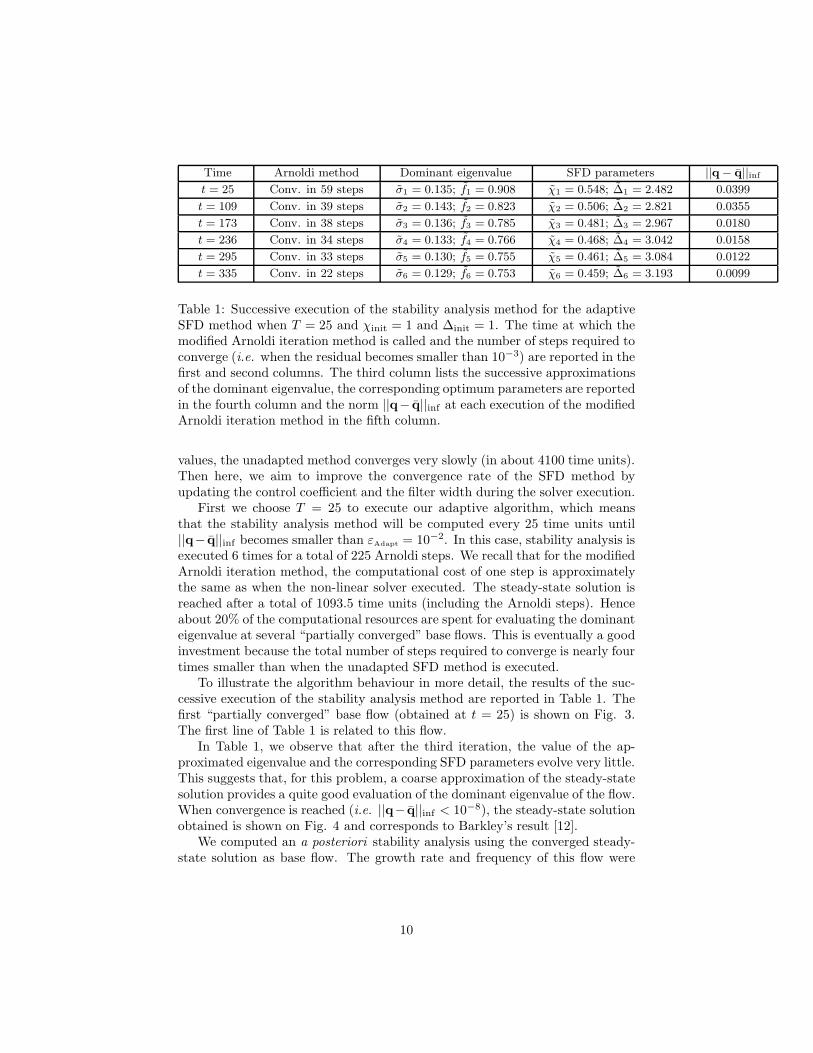
Table 1: Successive execution of the stability analysis method for the adaptiveSFD method when T = 25 and χinit = 1 and ∆init = 1. The time at which themodified Arnoldi iteration method is called and the number of steps required toconverge (i.e. when the residual becomes smaller than 10−3) are reported in thefirst and second columns. The third column lists the successive approximationsof the dominant eigenvalue, the corresponding optimum parameters are reportedin the fourth column and the norm ||q− q||inf at each execution of the modifiedArnoldi iteration method in the fifth column.

values, the unadapted method converges very slowly (in about 4100 time units).Then here, we aim to improve the convergence rate of the SFD method byupdating the control coefficient and the filter width during the solver execution.

First we choose T = 25 to execute our adaptive algorithm, which meansthat the stability analysis method will be computed every 25 time units until||q− q||inf becomes smaller than εAdapt = 10−2. In this case, stability analysis isexecuted 6 times for a total of 225 Arnoldi steps. We recall that for the modifiedArnoldi iteration method, the computational cost of one step is approximatelythe same as when the non-linear solver executed. The steady-state solution isreached after a total of 1093.5 time units (including the Arnoldi steps). Henceabout 20% of the computational resources are spent for evaluating the dominanteigenvalue at several “partially converged” base flows. This is eventually a goodinvestment because the total number of steps required to converge is nearly fourtimes smaller than when the unadapted SFD method is executed.

To illustrate the algorithm behaviour in more detail, the results of the suc-cessive execution of the stability analysis method are reported in Table 1. Thefirst “partially converged” base flow (obtained at t = 25) is shown on Fig. 3.The first line of Table 1 is related to this flow.

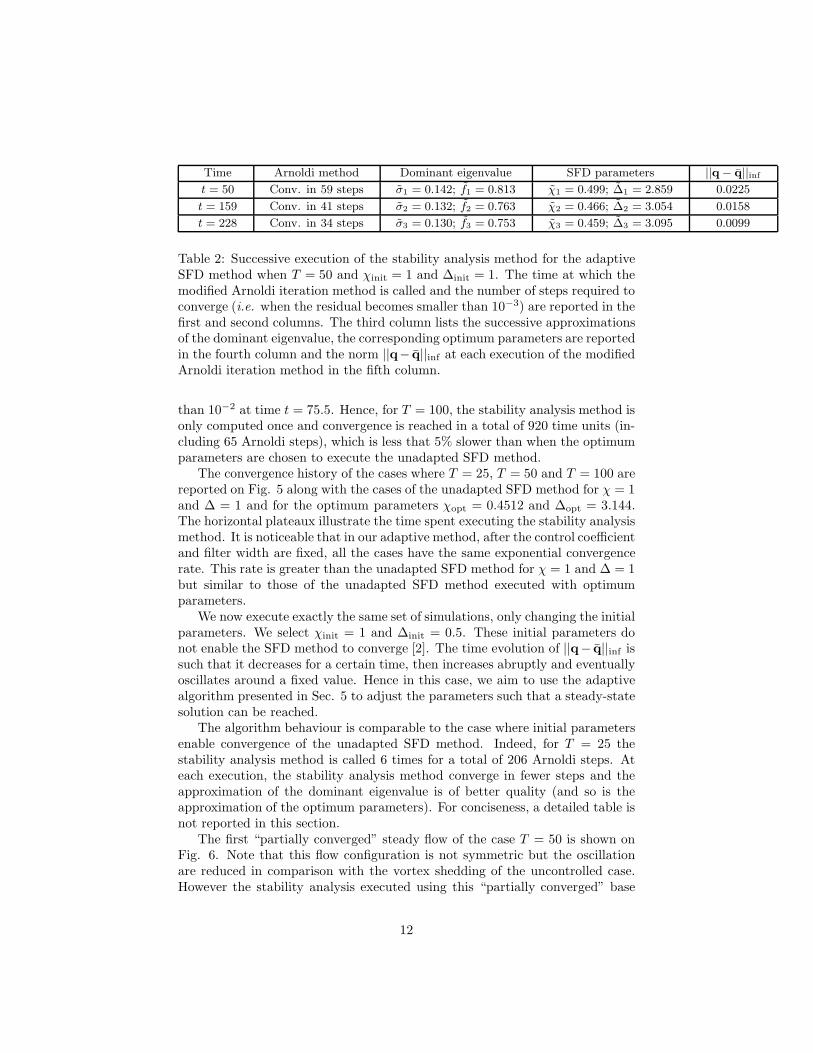
In Table 1, we observe that after the third iteration, the value of the ap-proximated eigenvalue and the corresponding SFD parameters evolve very little.This suggests that, for this problem, a coarse approximation of the steady-statesolution provides a quite good evaluation of the dominant eigenvalue of the flow.When convergence is reached (i.e. ||q− q||inf < 10−8), the steady-state solutionobtained is shown on Fig. 4 and corresponds to Barkley’s result [12].

We computed an a posteriori stability analysis using the converged steady-state solution as base flow. The growth rate and frequency of this flow were

10

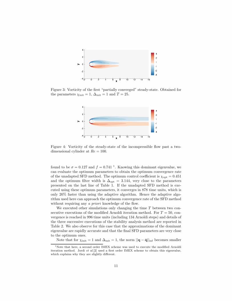
Figure 3: Vorticity of the first “partially converged” steady-state. Obtained forthe parameters χinit = 1, ∆init = 1 and T = 25.

Figure 4: Vorticity of the steady-state of the incompressible flow past a two-dimensional cylinder at Re = 100.

found to be σ = 0.127 and f = 0.741 1. Knowing this dominant eigenvalue, wecan evaluate the optimum parameters to obtain the optimum convergence rateof the unadapted SFD method. The optimum control coefficient is χopt = 0.451and the optimum filter width is ∆opt = 3.144, very close to the parameterspresented on the last line of Table 1. If the unadapted SFD method is exe-cuted using these optimum parameters, it converges in 878 time units, which isonly 20% faster than using the adaptive algorithm. Hence the adaptive algo-rithm used here can approach the optimum convergence rate of the SFD methodwithout requiring any a priori knowledge of the flow.

We executed other simulations only changing the time T between two con-secutive executions of the modified Arnoldi iteration method. For T = 50, con-vergence is reached in 996 time units (including 134 Arnoldi steps) and details ofthe three successive executions of the stability analysis method are reported inTable 2. We also observe for this case that the approximations of the dominanteigenvalue are rapidly accurate and that the final SFD parameters are very closeto the optimum ones.

Note that for χinit = 1 and ∆init = 1, the norm ||q− q||inf becomes smaller

1Note that here, a second order IMEX scheme was used to execute the modified Arnoldiiteration method. Jordi et al.[2] used a first order IMEX scheme to obtain this eigenvalue,which explains why they are slightly different.

11

Time Arnoldi method Dominant eigenvalue SFD parameters ||q− q||inf

t = 50 Conv. in 59 steps σ1 = 0.142; f1 = 0.813 χ1 = 0.499; ∆1 = 2.859 0.0225

t = 159 Conv. in 41 steps σ2 = 0.132; f2 = 0.763 χ2 = 0.466; ∆2 = 3.054 0.0158

t = 228 Conv. in 34 steps σ3 = 0.130; f3 = 0.753 χ3 = 0.459; ∆3 = 3.095 0.0099

Table 2: Successive execution of the stability analysis method for the adaptiveSFD method when T = 50 and χinit = 1 and ∆init = 1. The time at which themodified Arnoldi iteration method is called and the number of steps required toconverge (i.e. when the residual becomes smaller than 10−3) are reported in thefirst and second columns. The third column lists the successive approximationsof the dominant eigenvalue, the corresponding optimum parameters are reportedin the fourth column and the norm ||q− q||inf at each execution of the modifiedArnoldi iteration method in the fifth column.

than 10−2 at time t = 75.5. Hence, for T = 100, the stability analysis method isonly computed once and convergence is reached in a total of 920 time units (in-cluding 65 Arnoldi steps), which is less that 5% slower than when the optimumparameters are chosen to execute the unadapted SFD method.

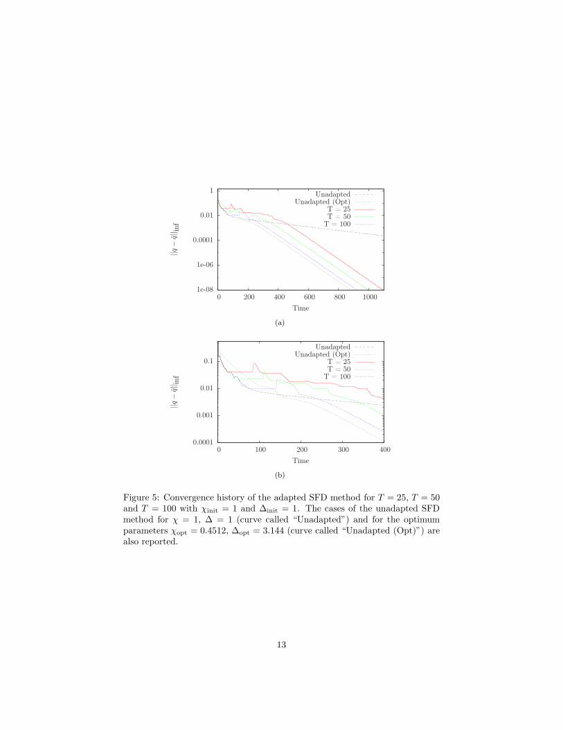
The convergence history of the cases where T = 25, T = 50 and T = 100 arereported on Fig. 5 along with the cases of the unadapted SFD method for χ = 1and ∆ = 1 and for the optimum parameters χopt = 0.4512 and ∆opt = 3.144.The horizontal plateaux illustrate the time spent executing the stability analysismethod. It is noticeable that in our adaptive method, after the control coefficientand filter width are fixed, all the cases have the same exponential convergencerate. This rate is greater than the unadapted SFD method for χ = 1 and ∆ = 1but similar to those of the unadapted SFD method executed with optimumparameters.

We now execute exactly the same set of simulations, only changing the initialparameters. We select χinit = 1 and ∆init = 0.5. These initial parameters donot enable the SFD method to converge [2]. The time evolution of ||q− q||inf issuch that it decreases for a certain time, then increases abruptly and eventuallyoscillates around a fixed value. Hence in this case, we aim to use the adaptivealgorithm presented in Sec. 5 to adjust the parameters such that a steady-statesolution can be reached.

The algorithm behaviour is comparable to the case where initial parametersenable convergence of the unadapted SFD method. Indeed, for T = 25 thestability analysis method is called 6 times for a total of 206 Arnoldi steps. Ateach execution, the stability analysis method converge in fewer steps and theapproximation of the dominant eigenvalue is of better quality (and so is theapproximation of the optimum parameters). For conciseness, a detailed table isnot reported in this section.

The first “partially converged” steady flow of the case T = 50 is shown onFig. 6. Note that this flow configuration is not symmetric but the oscillationare reduced in comparison with the vortex shedding of the uncontrolled case.However the stability analysis executed using this “partially converged” base

12

1e-08

1e-06

0.0001

0.01

1

0 200 400 600 800 1000

||q−

q|| inf

Time

UnadaptedUnadapted (Opt)

T = 25T = 50

T = 100

(a)

0.0001

0.001

0.01

0.1

0 100 200 300 400

||q−

q|| inf

Time

UnadaptedUnadapted (Opt)

T = 25T = 50

T = 100

(b)

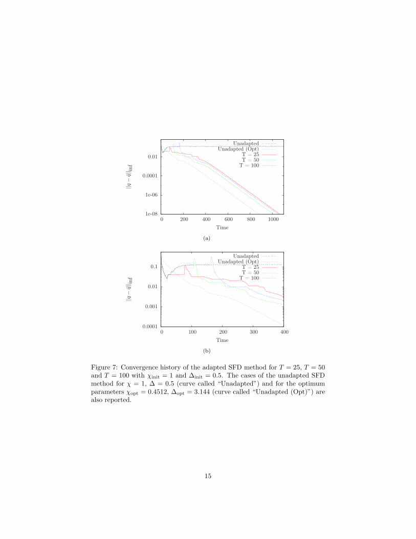
Figure 5: Convergence history of the adapted SFD method for T = 25, T = 50and T = 100 with χinit = 1 and ∆init = 1. The cases of the unadapted SFDmethod for χ = 1, ∆ = 1 (curve called “Unadapted”) and for the optimumparameters χopt = 0.4512, ∆opt = 3.144 (curve called “Unadapted (Opt)”) arealso reported.

13

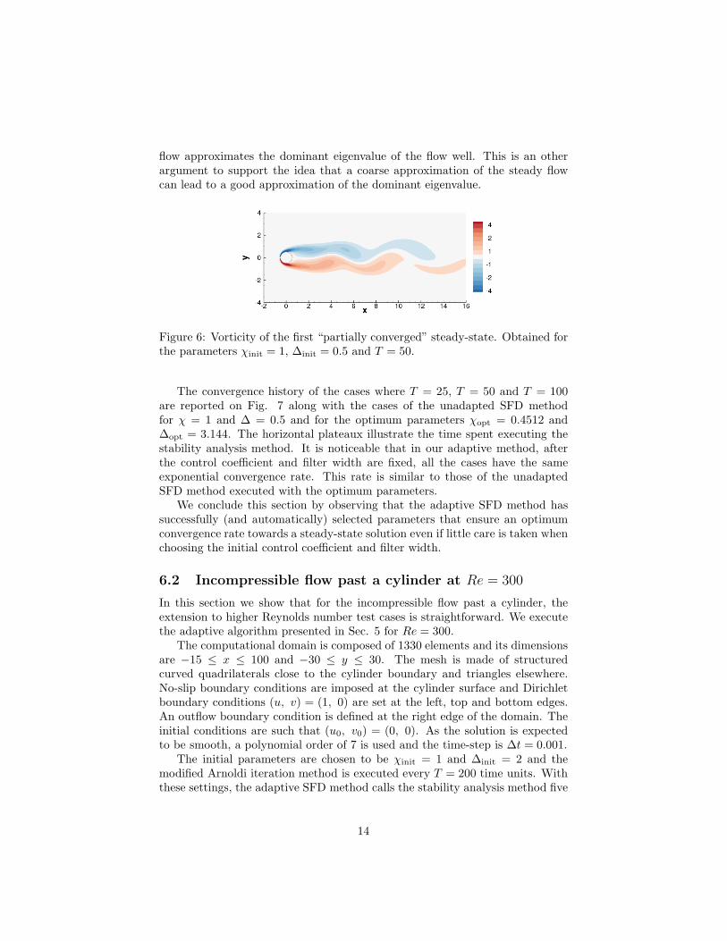
flow approximates the dominant eigenvalue of the flow well. This is an otherargument to support the idea that a coarse approximation of the steady flowcan lead to a good approximation of the dominant eigenvalue.

Figure 6: Vorticity of the first “partially converged” steady-state. Obtained forthe parameters χinit = 1, ∆init = 0.5 and T = 50.

The convergence history of the cases where T = 25, T = 50 and T = 100are reported on Fig. 7 along with the cases of the unadapted SFD methodfor χ = 1 and ∆ = 0.5 and for the optimum parameters χopt = 0.4512 and∆opt = 3.144. The horizontal plateaux illustrate the time spent executing thestability analysis method. It is noticeable that in our adaptive method, afterthe control coefficient and filter width are fixed, all the cases have the sameexponential convergence rate. This rate is similar to those of the unadaptedSFD method executed with the optimum parameters.

We conclude this section by observing that the adaptive SFD method hassuccessfully (and automatically) selected parameters that ensure an optimumconvergence rate towards a steady-state solution even if little care is taken whenchoosing the initial control coefficient and filter width.

6.2 Incompressible flow past a cylinder at Re = 300

In this section we show that for the incompressible flow past a cylinder, theextension to higher Reynolds number test cases is straightforward. We executethe adaptive algorithm presented in Sec. 5 for Re = 300.

The computational domain is composed of 1330 elements and its dimensionsare −15 ≤ x ≤ 100 and −30 ≤ y ≤ 30. The mesh is made of structuredcurved quadrilaterals close to the cylinder boundary and triangles elsewhere.No-slip boundary conditions are imposed at the cylinder surface and Dirichletboundary conditions (u, v) = (1, 0) are set at the left, top and bottom edges.An outflow boundary condition is defined at the right edge of the domain. Theinitial conditions are such that (u0, v0) = (0, 0). As the solution is expectedto be smooth, a polynomial order of 7 is used and the time-step is ∆t = 0.001.

The initial parameters are chosen to be χinit = 1 and ∆init = 2 and themodified Arnoldi iteration method is executed every T = 200 time units. Withthese settings, the adaptive SFD method calls the stability analysis method five

14

1e-08

1e-06

0.0001

0.01

0 200 400 600 800 1000

||q−

q|| inf

Time

UnadaptedUnadapted (Opt)

T = 25T = 50

T = 100

(a)

0.0001

0.001

0.01

0.1

0 100 200 300 400

||q−

q|| inf

Time

UnadaptedUnadapted (Opt)

T = 25T = 50

T = 100

(b)

Figure 7: Convergence history of the adapted SFD method for T = 25, T = 50and T = 100 with χinit = 1 and ∆init = 0.5. The cases of the unadapted SFDmethod for χ = 1, ∆ = 0.5 (curve called “Unadapted”) and for the optimumparameters χopt = 0.4512, ∆opt = 3.144 (curve called “Unadapted (Opt)”) arealso reported.

15

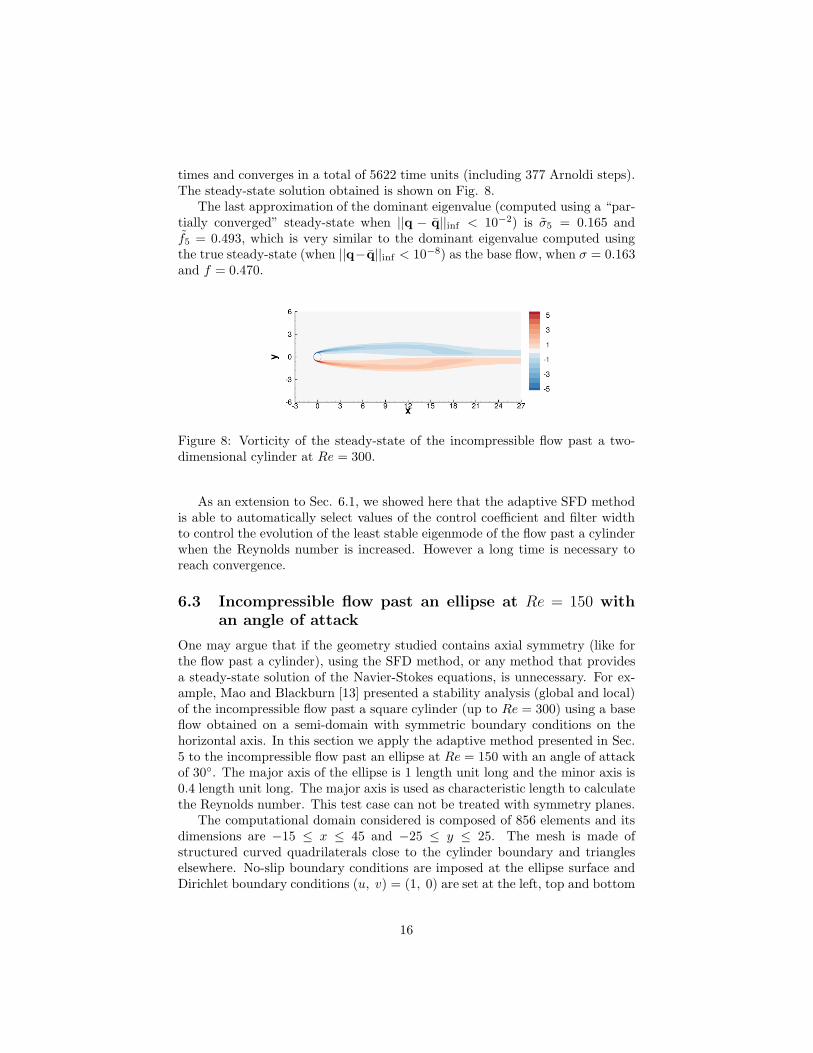
times and converges in a total of 5622 time units (including 377 Arnoldi steps).The steady-state solution obtained is shown on Fig. 8.

The last approximation of the dominant eigenvalue (computed using a “par-tially converged” steady-state when ||q − q||inf < 10−2) is σ5 = 0.165 andf5 = 0.493, which is very similar to the dominant eigenvalue computed usingthe true steady-state (when ||q−q||inf < 10−8) as the base flow, when σ = 0.163and f = 0.470.

Figure 8: Vorticity of the steady-state of the incompressible flow past a two-dimensional cylinder at Re = 300.

As an extension to Sec. 6.1, we showed here that the adaptive SFD methodis able to automatically select values of the control coefficient and filter widthto control the evolution of the least stable eigenmode of the flow past a cylinderwhen the Reynolds number is increased. However a long time is necessary toreach convergence.

6.3 Incompressible flow past an ellipse at Re = 150 with

an angle of attack

One may argue that if the geometry studied contains axial symmetry (like forthe flow past a cylinder), using the SFD method, or any method that providesa steady-state solution of the Navier-Stokes equations, is unnecessary. For ex-ample, Mao and Blackburn [13] presented a stability analysis (global and local)of the incompressible flow past a square cylinder (up to Re = 300) using a baseflow obtained on a semi-domain with symmetric boundary conditions on thehorizontal axis. In this section we apply the adaptive method presented in Sec.5 to the incompressible flow past an ellipse at Re = 150 with an angle of attackof 30◦. The major axis of the ellipse is 1 length unit long and the minor axis is0.4 length unit long. The major axis is used as characteristic length to calculatethe Reynolds number. This test case can not be treated with symmetry planes.

The computational domain considered is composed of 856 elements and itsdimensions are −15 ≤ x ≤ 45 and −25 ≤ y ≤ 25. The mesh is made ofstructured curved quadrilaterals close to the cylinder boundary and triangleselsewhere. No-slip boundary conditions are imposed at the ellipse surface andDirichlet boundary conditions (u, v) = (1, 0) are set at the left, top and bottom

16

edges. An outflow boundary condition is defined at the right edge of the domain.The initial conditions are such that (u0, v0) = (0, 0). A polynomial order of 7is used and the time-step is ∆t = 0.0025.

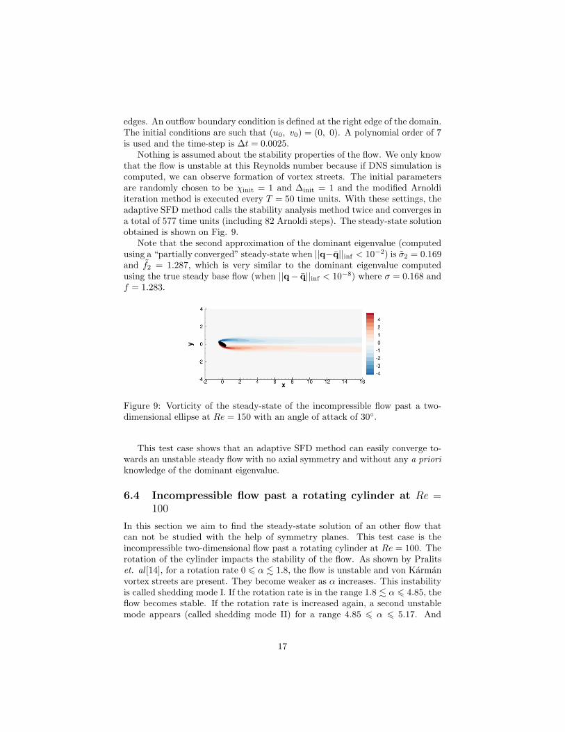
Nothing is assumed about the stability properties of the flow. We only knowthat the flow is unstable at this Reynolds number because if DNS simulation iscomputed, we can observe formation of vortex streets. The initial parametersare randomly chosen to be χinit = 1 and ∆init = 1 and the modified Arnoldiiteration method is executed every T = 50 time units. With these settings, theadaptive SFD method calls the stability analysis method twice and converges ina total of 577 time units (including 82 Arnoldi steps). The steady-state solutionobtained is shown on Fig. 9.

Note that the second approximation of the dominant eigenvalue (computedusing a “partially converged” steady-state when ||q−q||inf < 10−2) is σ2 = 0.169and f2 = 1.287, which is very similar to the dominant eigenvalue computedusing the true steady base flow (when ||q− q||inf < 10−8) where σ = 0.168 andf = 1.283.

Figure 9: Vorticity of the steady-state of the incompressible flow past a two-dimensional ellipse at Re = 150 with an angle of attack of 30◦.

This test case shows that an adaptive SFD method can easily converge to-wards an unstable steady flow with no axial symmetry and without any a prioriknowledge of the dominant eigenvalue.

6.4 Incompressible flow past a rotating cylinder at Re =

100

In this section we aim to find the steady-state solution of an other flow thatcan not be studied with the help of symmetry planes. This test case is theincompressible two-dimensional flow past a rotating cylinder at Re = 100. Therotation of the cylinder impacts the stability of the flow. As shown by Pralitset. al [14], for a rotation rate 0 6 α . 1.8, the flow is unstable and von Karmanvortex streets are present. They become weaker as α increases. This instabilityis called shedding mode I. If the rotation rate is in the range 1.8 . α 6 4.85, theflow becomes stable. If the rotation rate is increased again, a second unstablemode appears (called shedding mode II) for a range 4.85 6 α 6 5.17. And

17

eventually, for rotation rates above 5.17, the flow is stable. Note that thisbehaviour is only true in two-dimensions. In three-dimensions the presence ofshedding mode I and the range of shedding mode II depend on the spanwisewave number[15].

Here we are interested in finding a steady-state solution of the unstablemode II, hence we consider a rotation rate α = 5. The computational domainconsidered is composed of 1044 elements and its dimensions are −15 ≤ x ≤ 45and −25 ≤ y ≤ 25. The mesh is made of structured curved quadrilaterals closeto the cylinder boundary and triangles elsewhere. The mesh is fine close to thecylinder boundary because its rotation induces a strong velocity gradient. Also,the region on the right of the cylinder and for 0 ≤ y ≤ 8 is refined becausethat is where the shedding vortices appear when a DNS simulation is executed.Slip boundary conditions are imposed at the cylinder surface such that u·t =α and u·n = 0, where u is the velocity vector, t and n are the tangentialand normal vectors to the surface respectively. Dirichlet boundary conditions(u, v) = (1, 0) are set at the left, top and bottom edges. An outflow boundarycondition is defined at the right edge of the domain. The initial conditions aresuch that (u0, v0) = (0, 0). A polynomial order of 7 is used and the time-stepis ∆t = 0.0005.

To compute the adaptive method presented in Sec. 5, the initial controlcoefficient of the SFD method is randomly chosen to be χinit = 1. However somecare is taken to the selection of the initial filter width. When DNS simulationis executed, we observe that the frequency of the shedding mode II is very low.Thus the initial filter width of the SFD method must be chosen to be quite high,e.g. ∆init = 5. Larger filter widths enable us to control instabilities that arise ona larger time scale, but may require an impractically long time to converge. TheSFD method is well suited to obtain steady-state solutions of flows with highunstable frequencies. Hence the flow past a cylinder at the unstable sheddingmode II is challenging for the SFD method. For this test case the initial filterwidth is carefully chosen, but nothing is assumed about the dominant eigenvalueof the flow.

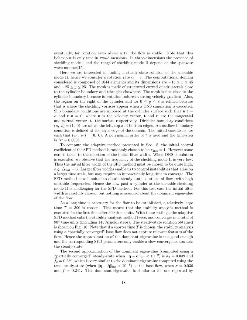
As a long time is necessary for the flow to be established, a relatively largetime T = 300 is chosen. This means that the stability analysis method isexecuted for the first time after 300 time units. With these settings, the adaptiveSFD method calls the stability analysis method twice, and converges in a total of907 time units (including 145 Arnoldi steps). The steady-state solution obtainedis shown on Fig. 10. Note that if a shorter time T is chosen, the stability analysisusing a “partially converged” base flow does not capture relevant features of theflow. Hence the approximation of the dominant eigenvalue is not good enoughand the corresponding SFD parameters only enable a slow convergence towardsthe steady-state.

The second approximation of the dominant eigenvalue (computed using a“partially converged” steady-state when ||q − q||inf < 10−2) is σ2 = 0.039 andf2 = 0.239, which is very similar to the dominant eigenvalue computed using thetrue steady-state (when ||q − q||inf < 10−8) as the base flow, when σ = 0.036and f = 0.241. This dominant eigenvalue is similar to the one reported by

18

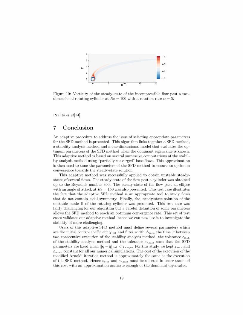
Figure 10: Vorticity of the steady-state of the incompressible flow past a two-dimensional rotating cylinder at Re = 100 with a rotation rate α = 5.

Pralits et al [14].

7 Conclusion

An adaptive procedure to address the issue of selecting appropriate parametersfor the SFD method is presented. This algorithm links together a SFD method,a stability analysis method and a one-dimensional model that evaluates the op-timum parameters of the SFD method when the dominant eigenvalue is known.This adaptive method is based on several successive computations of the stabil-ity analysis method using “partially converged” base flows. This approximationis then used to tune the parameters of the SFD method to ensure an optimumconvergence towards the steady-state solution.

This adaptive method was successfully applied to obtain unstable steady-states of several flows. The steady-state of the flow past a cylinder was obtainedup to the Reynolds number 300. The steady-state of the flow past an ellipsewith an angle of attack at Re = 150 was also presented. This test case illustratesthe fact that the adaptive SFD method is an appropriate tool to study flowsthat do not contain axial symmetry. Finally, the steady-state solution of theunstable mode II of the rotating cylinder was presented. This test case wasfairly challenging for our algorithm but a careful definition of some parametersallows the SFD method to reach an optimum convergence rate. This set of testcases validates our adaptive method, hence we can now use it to investigate thestability of more challenging.

Users of this adaptive SFD method must define several parameters whichare the initial control coefficient χinit and filter width ∆init, the time T betweentwo consecutive execution of the stability analysis method, the tolerance εStab

of the stability analysis method and the tolerance εAdapt such that the SFDparameters are fixed when ||q− q||inf < εAdapt. For this study we kept εStab andεAdapt constant for all our numerical simulations. The cost of the execution of themodified Arnoldi iteration method is approximately the same as the executionof the SFD method. Hence εStab and εAdapt must be selected in order trade-offthis cost with an approximation accurate enough of the dominant eigenvalue.

19

For all our simulations, the steady-state solution was found in several hun-dreds time units (several thousands for some cases). Even if the convergencerate of the SFD method is optimal, the time (and the computational cost) nec-essary to reach the steady-state solution may still be important. It may be thatthe adaptive SFD method could be then used as a global solver to find an initialguess of a Newton’s method. This might allow us to design algorithms capableof reaching unstable steady-state solutions in a limited number of iterations.

Acknowledgments

The authors would like to thank the Seventh Framework Programme of theEuropean Commission for their support to the ANADE project (Advances inNumerical and Analytical tools for DEtached flow prediction) under grant con-tract PITN-GA-289428.

References

[1] E. Akervik, L. Brandt, D. S. Henningson, J. Hœpffner, O. Marxen, andP. Schlatter. Steady solutions of the Navier-Stokes equations by selectivefrequency damping. Phys. Fluids, 18, 2006.

[2] B. E. Jordi, C. J. Cotter, and S. J. Sherwin. Encapsulated formulation ofthe selective frequency damping method. Phys. Fluids, 26, 2014.

[3] S. J. Sherwin and H. M. Blackburn. Three-dimensional instabilities andtransition of steady and pulsatile axisymmetric stenotic flows. J. FluidMech., 533:297–327, 2005.

[4] D. Barkley, H. M. Blackburn, and S. J. Sherwin. Direct optimal growthanalysis for timesteppers. Int. J. Numer. Meth. Fl., 57(9):1435–1458, 2008.

[5] I. Farago. Splitting methods and their application to the abstract Cauchyproblems. In Numerical Analysis and Its Applications, pages 35–45.Springer, 2005.

[6] L. Tuckerman and D. Barkley. Bifurcation analysis for timesteppers. Nu-merical methods for bifurcation problems and large-scale dynamical system,pages 453–566, 2000.

[7] Nektar++. http://www.nektar.info, 2014.

[8] Gabriele Rocco. Advanced Instability Methods using Spectral/hp Discretisa-tions and their Applications to Complex Geometries. PhD thesis, ImperialCollege London, 2014.

[9] R. B. Lehoucq, D. C. Sorensen, and C. Yang. ARPACK users’ guide:solution of large-scale eigenvalue problems with implicitly restarted Arnoldimethods, volume 6. Siam, 1998.

20

[10] G. E. Karniadakis and S. J. Sherwin. Spectral/hp Element Methods forCFD. Oxford University Press, second edition, 2005.

[11] U. M. Ascher, S. J. Ruuth, and B. T. R. Wetton. Implicit-explicit methodsfor time-dependent partial differential equations. SIAM J. Numer. Anal.,32(3):797–823, 1995.

[12] D. Barkley. Linear analysis of the cylinder wake mean flow. EPL (Euro-physics Letters), 75(12):750, 2006.

[13] X. Mao and H. M. Blackburn. The structure of primary instability modesin the steady wake and separation bubble of a square cylinder. Phys. Fluids,26(7):074103, 2014.

[14] J. O. Pralits, L. Brandt, and F. Giannetti. Instability and sensitivity ofthe flow around a rotating circular cylinder. J. Fluid Mech., 650:513–536,2010.

[15] J. O. Pralits, F. Giannetti, and L. Brandt. Three-dimensional instabilityof the flow around a rotating circular cylinder. J. Fluid Mech., 730:5–18,2013.

21