Regression Estimation - Least Squares andMaximum Likelihood

Dr. Frank Wood

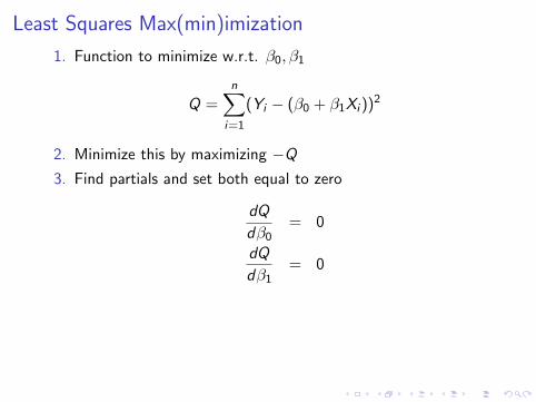
Least Squares Max(min)imization

1. Function to minimize w.r.t. β0, β1

Q =n∑

i=1

(Yi − (β0 + β1Xi ))2

2. Minimize this by maximizing −Q

3. Find partials and set both equal to zero

dQ

dβ0= 0

dQ

dβ1= 0

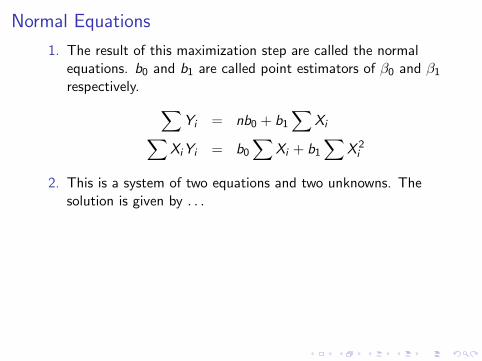
Normal Equations

1. The result of this maximization step are called the normalequations. b0 and b1 are called point estimators of β0 and β1

respectively. ∑Yi = nb0 + b1

∑Xi∑

XiYi = b0

∑Xi + b1

∑X 2

i

2. This is a system of two equations and two unknowns. Thesolution is given by . . .

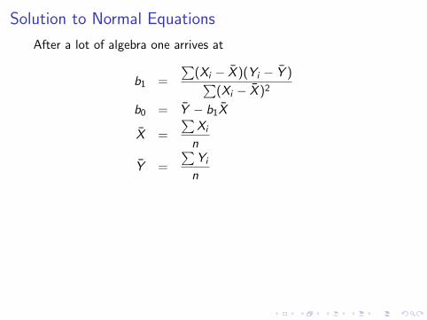
Solution to Normal Equations

After a lot of algebra one arrives at

b1 =

∑(Xi − X )(Yi − Y )∑

(Xi − X )2

b0 = Y − b1X

X =

∑Xi

n

Y =

∑Yi

n

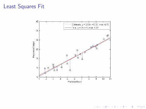
Least Squares Fit

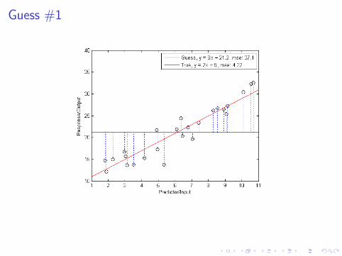
Guess #1

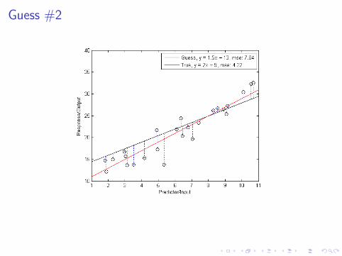
Guess #2

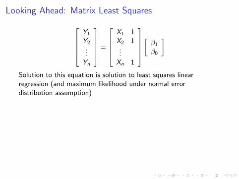
Looking Ahead: Matrix Least Squares

Y1

Y2...

Yn

=

X1 1X2 1...

Xn 1

[β1

β0

]

Solution to this equation is solution to least squares linearregression (and maximum likelihood under normal errordistribution assumption)

Questions to Ask

1. Is the relationship really linear?

2. What is the distribution of the of “errors”?

3. Is the fit good?

4. How much of the variability of the response is accounted forby including the predictor variable?

5. Is the chosen predictor variable the best one?

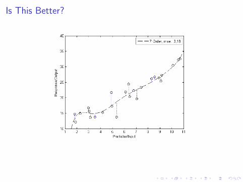
Is This Better?

Goals for First Half of Course

1. How to do linear regression

1.1 Self familiarization with software tools

2. How to interpret standard linear regression results

3. How to derive tests

4. How to assess and address deficiencies in regression models

Estimators for β0, β1, σ2

1. We want to establish properties of estimators for β0, β1, andσ2 so that we can construct hypothesis tests and so forth

2. We will start by establishing some properties of the regressionsolution.

Properties of Solution

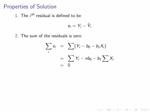
1. The i th residual is defined to be

ei = Yi − Yi

2. The sum of the residuals is zero:∑i

ei =∑

(Yi − b0 − b1Xi )

=∑

Yi − nb0 − b1

∑Xi

= 0

Properties of Solution

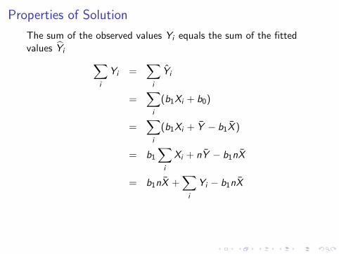
The sum of the observed values Yi equals the sum of the fittedvalues Yi ∑

i

Yi =∑

i

Yi

=∑

i

(b1Xi + b0)

=∑

i

(b1Xi + Y − b1X )

= b1

∑i

Xi + nY − b1nX

= b1nX +∑

i

Yi − b1nX

Properties of Solution

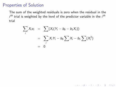
The sum of the weighted residuals is zero when the residual in thei th trial is weighted by the level of the predictor variable in the i th

trial ∑i

Xiei =∑

(Xi (Yi − b0 − b1Xi ))

=∑

i

XiYi − b0

∑Xi − b1

∑(X 2

i )

= 0

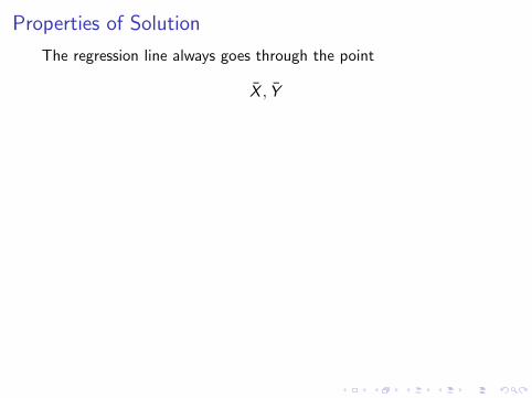
Properties of Solution

The regression line always goes through the point

X , Y

Estimating Error Term Variance σ2

1. Review estimation in non-regression setting.

2. Show estimation results for regression setting.

Estimation Review

1. An estimator is a rule that tells how to calculate the value ofan estimate based on the measurements contained in a sample

2. i.e. the sample mean

Y =1

n

n∑i=1

Yi

Point Estimators and Bias

1. Point estimatorθ = f ({Y1, . . . ,Yn})

2. Unknown quantity / parameter

θ

3. Definition: Bias of estimator

B(θ) = E(θ)− θ

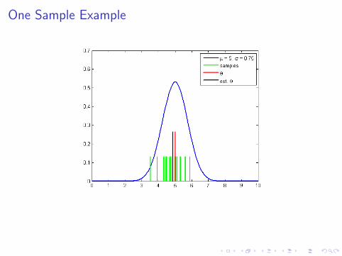
One Sample Example

Distribution of Estimator

1. If the estimator is a function of the samples and thedistribution of the samples is known then the distribution ofthe estimator can (often) be determined1.1 Methods

1.1.1 Distribution (CDF) functions1.1.2 Transformations1.1.3 Moment generating functions1.1.4 Jacobians (change of variable)

Example

1. Samples from a Normal(µ, σ2) distribution

Yi ∼ Normal(µ, σ2)

2. Estimate the population mean

θ = µ, θ = Y =1

n

n∑i=1

Yi

Sampling Distribution of the Estimator

1. First moment

E (θ) = E (1

n

n∑i=1

Yi )

=1

n

n∑i=1

E (Yi ) =nµ

n= θ

2. This is an example of an unbiased estimator

B(θ) = E (θ)− θ = 0

Variance of Estimator

1. Definition: Variance of estimator

V (θ) = E ([θ − E (θ)]2)

2. Remember:

V (cY ) = c2V (Y )

V (n∑

i=1

Yi ) =n∑

i=1

V (Yi )

Only if the Yi are independent with finite variance

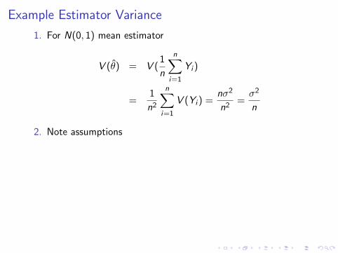
Example Estimator Variance

1. For N(0, 1) mean estimator

V (θ) = V (1

n

n∑i=1

Yi )

=1

n2

n∑i=1

V (Yi ) =nσ2

n2=σ2

n

2. Note assumptions

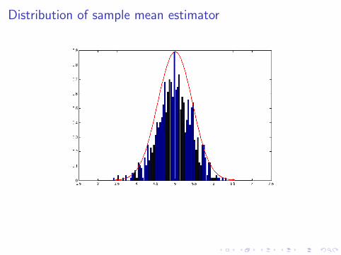
Distribution of sample mean estimator

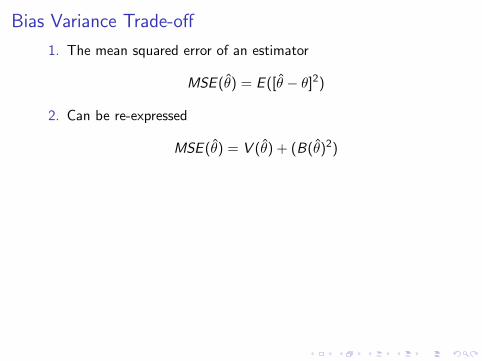
Bias Variance Trade-off

1. The mean squared error of an estimator

MSE (θ) = E ([θ − θ]2)

2. Can be re-expressed

MSE (θ) = V (θ) + (B(θ)2)

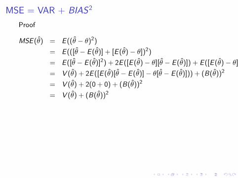
MSE = VAR + BIAS2

Proof

MSE (θ) = E ((θ − θ)2)

= E (([θ − E (θ)] + [E (θ)− θ])2)

= E ([θ − E (θ)]2) + 2E ([E (θ)− θ][θ − E (θ)]) + E ([E (θ)− θ]2)

= V (θ) + 2E ([E (θ)[θ − E (θ)]− θ[θ − E (θ)])) + (B(θ))2

= V (θ) + 2(0 + 0) + (B(θ))2

= V (θ) + (B(θ))2

Trade-off

1. Think of variance as confidence and bias as correctness.

1.1 Intuitions (largely) apply

2. Sometimes a biased estimator can produce lower MSE if itlowers the variance.

Estimating Error Term Variance σ2

1. Regression model

2. Variance of each observation Yi is σ2 (the same as for theerror term εi )

3. Each Yi comes from a different probability distribution withdifferent means that depend on the level Xi

4. The deviation of an observation Yi must be calculated aroundits own estimated mean.

s2 estimator for σ2

s2 = MSE =SSE

n − 2=

∑(Yi − Yi )

2

n − 2=

∑e2i

n − 2

1. MSE is an unbiased estimator of σ2

E (MSE ) = σ2

2. The sum of squares SSE has n-2 degrees of freedomassociated with it.

Normal Error Regression Model

1. No matter how the error terms εi are distributed, the leastsquares method provides unbiased point estimators of β0 andβ1

1.1 that also have minimum variance among all unbiased linearestimators

2. To set up interval estimates and make tests we need tospecify the distribution of the εi

3. We will assume that the εi are normally distributed.

Normal Error Regression Model

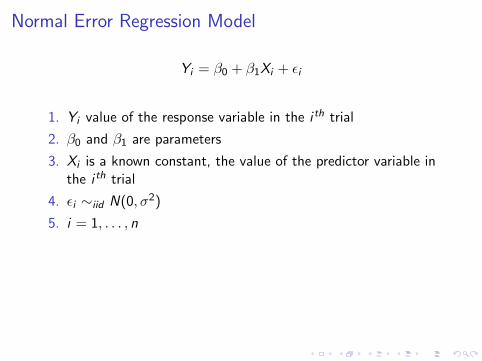
Yi = β0 + β1Xi + εi

1. Yi value of the response variable in the i th trial

2. β0 and β1 are parameters

3. Xi is a known constant, the value of the predictor variable inthe i th trial

4. εi ∼iid N(0, σ2)

5. i = 1, . . . , n

Notational Convention

1. When you see εi ∼iid N(0, σ2)

2. It is read as εi is distributed identically and independentlyaccording to a normal distribution with mean 0 and varianceσ2

3. Examples

3.1 θ ∼ Poisson(λ)3.2 z ∼ G (θ)

Maximum Likelihood Principle

The method of maximum likelihood chooses as estimates thosevalues of the parameters that are most consistent with the sampledata.

Likelihood Function

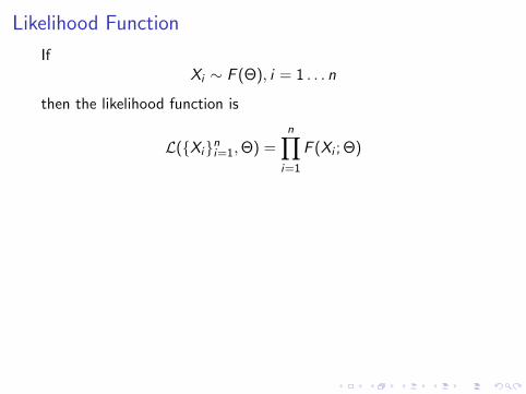
IfXi ∼ F (Θ), i = 1 . . . n

then the likelihood function is

L({Xi}ni=1,Θ) =n∏

i=1

F (Xi ; Θ)

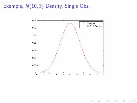
Example, N(10, 3) Density, Single Obs.

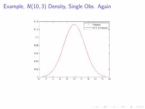
Example, N(10, 3) Density, Single Obs. Again

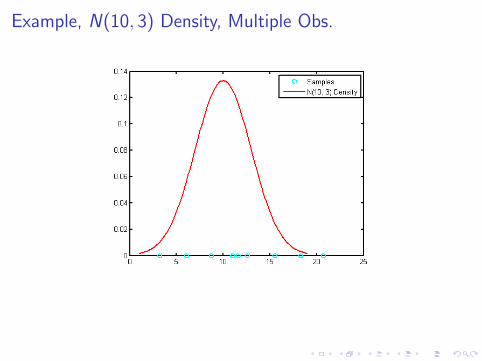
Example, N(10, 3) Density, Multiple Obs.

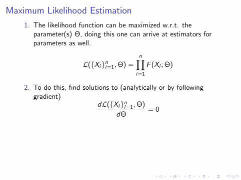
Maximum Likelihood Estimation

1. The likelihood function can be maximized w.r.t. theparameter(s) Θ, doing this one can arrive at estimators forparameters as well.

L({Xi}ni=1,Θ) =n∏

i=1

F (Xi ; Θ)

2. To do this, find solutions to (analytically or by followinggradient)

dL({Xi}ni=1,Θ)

dΘ= 0

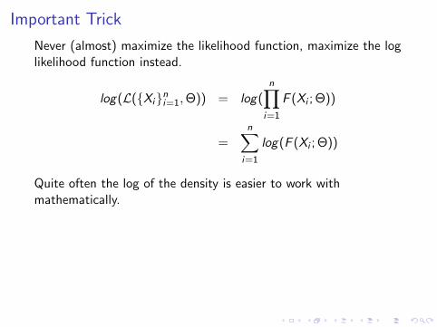
Important Trick

Never (almost) maximize the likelihood function, maximize the loglikelihood function instead.

log(L({Xi}ni=1,Θ)) = log(n∏

i=1

F (Xi ; Θ))

=n∑

i=1

log(F (Xi ; Θ))

Quite often the log of the density is easier to work withmathematically.

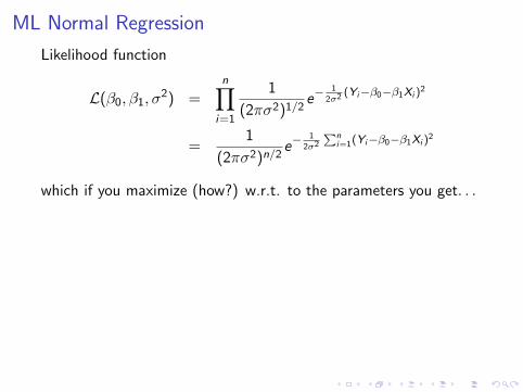
ML Normal Regression

Likelihood function

L(β0, β1, σ2) =

n∏i=1

1

(2πσ2)1/2e−

12σ2 (Yi−β0−β1Xi )

2

=1

(2πσ2)n/2e−

12σ2

Pni=1(Yi−β0−β1Xi )

2

which if you maximize (how?) w.r.t. to the parameters you get. . .

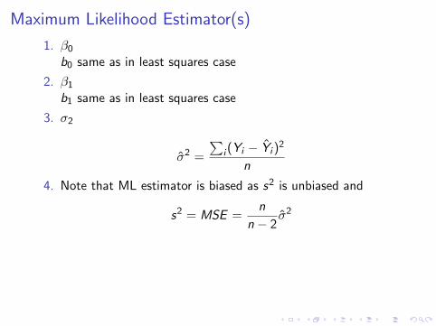
Maximum Likelihood Estimator(s)

1. β0

b0 same as in least squares case

2. β1

b1 same as in least squares case

3. σ2

σ2 =

∑i (Yi − Yi )

2

n

4. Note that ML estimator is biased as s2 is unbiased and

s2 = MSE =n

n − 2σ2

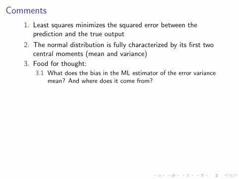
Comments

1. Least squares minimizes the squared error between theprediction and the true output

2. The normal distribution is fully characterized by its first twocentral moments (mean and variance)

3. Food for thought:

3.1 What does the bias in the ML estimator of the error variancemean? And where does it come from?