Online investors’ trading behaviour and performance:

Evidence from the Korean equity market

NATALIE Y OH* Ψ

University of New South Wales and SIRCA Limited

JERRY T PARWADA*

University of New South Wales and SIRCA Limited

TERRY S WALTER*

University of New South Wales and Capital Markets CRC Limited

Abstract This paper investigates the trading behaviour and performance of online equity investors in comparison to other investors on the Korean stock market. We find that online traders are noise traders who provide liquidity to other investors. We also show that the aggregate trading activity of all investor types largely fails to explain market returns. However, returns on the index have a significant positive impact in changing online investment flows, compared to the negative feedback trading we find for other domestic investor types. Volatility is apparently perceived as an opportunity, and like all other investors, online traders increase their trading during volatile periods. In periods when there is uncertainty about the future direction of the market online investors reduce purchases and sales indiscriminately. Although some market timing ability characterizes online buy trades, the long run performance of online investors’ trading decisions is below that of other investor types.

JEL classification: G10; G20; O33

Key words: Online trading, Performance, Investor Behaviour

*We thank the Securities Industry Research Centre of Asia Pacific for financial support and acknowledge Mr Youngjin Kim from KSDA for valuable comments. Mr Kilhyun Ahn from the Korean Stock Exchange gets special thanks for providing data. Ψ Corresponding author. Address for correspondence: SIRCA Research, PO Box H58 Australia Square, NSW 1215, Australia. Telephone: +61 2 9236 9118, Fax: +61 2 9231 5988 E-mail. natalie@sirca.org.au (Oh); jerry@sirca.org.au (Parwada); t.walter@unsw.edu.au (Walter)

1. Introduction

Recent developments in internet-based transaction technologies have allowed online

investing to become an important, if not controversial, feature of financial markets.1

Online trading has the potential to lower transaction costs and facilitate entry, resulting in

increased trading volumes (D’Avolio, Gildor, and Schleifer, 2002). Despite evidence

that internet-based stock trading now accounts for a large proportion of securities trading,

it is surprising that very few academic studies have been conducted of this rapidly

expanding form of trading. Choi, Laibson, and Metrick (2002) and Barber and Odean

(2002) are the exceptions. Choi et. al compare online traders with phone-based traders

using a sample of 100,000 members of two large US pension funds, and find that the

availability of internet trading increases transactions by 50 percent. Barber and Odean

document increased trading activity and a higher propensity to speculate amongst

investors who take up online trading. Importantly, these studies show that trading profits

quickly deteriorate (Barber and Odean) or are non-existent (Choi, Liabson and Metrick)

in the period after online trading is adopted.

Online investing research is of interest from at least two perspectives. First, by

demonstrating that online trading increases volume, these studies open up the possibility

that online investing may bring price pressure to bear in markets. Second, by analyzing

post trading performance, it can be deduced whether the phenomenal growth in volume is

driven by information or cognitive biases on the part of the investors.

1 See (Barber and Odean, 2002) for US data and examples of adverse press coverage of online trading.

1

In this paper we examine the behaviour and performance of online investors, and

compare this to other investor categories in the Korean equity market. We choose this

market because the level of online investing in Korea may be characterized as being

phenomenal. For example, online trading accounted for 65.3 percent of all stock trading

on Korean Stock Exchange (KSE) in April 2003. We examine the behaviour of

aggregated online trading to identify any systematic patterns that emerge relative to other

investors. To the best of our knowledge this paper represents the first substantive study

that directly compares online investors’ behaviour and performance to all other

participants in the equity market. The study closest to ours is Jackson (2003). He uses

individual client accounts at a sample of 56 Australian retail stockbroking firms,

including nine internet brokers, to investigate whether discernible flow-return patterns

exist for his dataset. The average trade size is $7,570 for internet brokerage clients, and

$10,080 for the full-service brokers, suggesting that Jackson’s study does not capture

much of the institutional trading on ASX.

We utilize a detailed database of daily trading volumes and values provided by the KSE.

Importantly this database links volumes and values to each of the categories of investors

originating the trades, including online investors, individual investors, foreign investors,

local institutional investors, securities houses and unclassified institutional investors.

Such data are not readily available in other markets. This makes our study a potentially

useful supplement to the studies that have used proprietary firm level data.2 Moreover,

2 Barber and Odean (2002) use a dataset consisting of clients of a discount brokerage firm; Choi, Laibson

and Metrick (2002) utilise data on two US pension funds.

2

the dataset splits trades into purchases and sales allowing us to augment our approach

with analysis based on trade imbalances, as aggregate trading activity could mask

interesting trading traits.

This paper is organized as follows. The next section summarizes the background to

online trading and the related literature and Section 3 describes the data and market

setting. Trading behaviour and performance are analyzed in Sections 4 and 5,

respectively. Section 6 concludes.

2. Background to perceptions of online investors

This section reviews the role of internet investing and the research literature relevant to

this paper.

The benefits for online trading have been documented in various industries. For

example, Brown and Goolsbee (2002) suggest that the internet may significantly reduce

search costs by enabling price comparisons online in the insurance market. However, it

is not clear that informational advantages translate into superior return performance in

equity markets. Barber and Odean (2002) investigate the performance of investors who

switched from phone-based trading to internet trading. While those traders who opted for

internet trading initially beat the market by about 2% prior to going online, their

performance decreased afterwards, resulting in performance 3% below the market. Choi,

Laibson and Metrick (2002) also report evidence of underperformance in the market

3

timing of online traders in a 401(k) plan.3 Thus, access to wider information sources on

the internet does not seem to imply higher return performance.

Whilst online investing facilities may have reduced the costs of trading, there is a

downside. First, the detrimental effects of high portfolio turnover have been shown to

reduce performance (Barber and Odean, 2000, 2002 and Choi Laibson and Metrick,

2002).4 In contrast, additional trading increases liquidity and this may induce even

higher volumes, possibly creating a “winner’s curse”. Second, trading volume “bubbles”

in online trading may result in another detrimental feature - low information revelation.

Third, online trading may also increase noise as information sources such as discussion

groups (dominated by unsophisticated investors) become an avenue for spreading

inaccurate information (Madhavan, 2000). According to D’Avolio, Gildor and Shleifer

(2001), “A well functioning securities market relies on the availability of accurate

information, a broad base of investors who can process this information, legal protection

of these investors’ rights, and a liquid secondary market unencumbered by excessive

transaction costs and constraints.”

The reliance of securities markets on a broad base of investors who can process

information has been considered questionable in the case of online investors. Are online

3 401(k) plans are the primary vehicle for retirement savings in the United States. According to Choi,

Laibson and Metrick (2002), in 1999, 401(k) plans held $1.6 trillion in assets, 72% of which represent

equity holdings.

4 See also Carhart (1997) on the negative relation between portfolio turnover and net returns in mutual

funds.

4

investors able to process information correctly and thus contribute to a well-functioning

market? Recently, online trading has been criticized in the financial press as being a

conduit for introducing unsophisticated individuals into the market, thus making the

market too speculative in ways synonymous with a gambling arena.5 The justification

behind this accusation is that it is believed the so-called inexperienced online traders have

access to an overwhelming amount of information through the internet, which creates an

illusion of knowledge and brings about overconfidence in trading (Barber and Odean,

2002). Further, lower transaction costs with online trading have allowed online investors

to engage in speculative trading more cheaply, thus creating speculative bubbles,

inducing higher volatility, asset mispricing and poor trading performance.6

It is surprising, given the contentious perceptions of online investors’ behaviour, that

there has not been any systematic analysis of the aggregate behaviour and trading returns

for online investors. We provide empirical evidence on these issues and, perhaps more

importantly, compare online investors’ behaviour with other investors to identify whether

internet-based traders indeed behave in a manner that warrants such criticism.

5 See for example, “Digital Manipulation” The Economist, 10th February 2001 (on the Korean market);

“Online Trading May Trigger New Dimension in Volatility” New Straits Times Press, 19th October 2000

(Malaysia); and “Technology Boom Keeps Volatility Ticking”; Australian Financial Review, 28th August

2000 (Australia).

6 See Barber and Odean (2001) for a review of the experimental economics literature on asset bubbles.

5

3. Data and market background

3.1. Data

This paper utilizes daily data on online trading volumes obtained from the KSE. The data

identify trading volume (number of shares traded) and value (Korean won) for both

purchases and sales over the 2001-2003 period. The sample period falls after the

worldwide “tech boom” which started in 1999 and the subsequent “tech bust” which

diminished in late 2000.

The dataset provides information on aggregate online trading activity that is not readily

available in other equity markets. The dataset also contains trading volumes and values

for other market participants. These include foreign investors (hereafter denoted

Foreigners), individual investors (Individuals), local institutional investors (Institutions),

securities houses (Securities) and unclassified institutions (Others).7 Institutions

comprise insurance, investment trust companies, commercial banks, merchant banks and

pension funds. Securities are the local securities companies that trade on their own

behalf (principal trading). Others in the dataset are mainly government agencies. We

exclude Others from this study because they trade infrequently. Others have also been 7 The foreign investor category includes both institutional and individual investors, but most trades are

from institutions. It is possible that trades we identify as foreign trades are actually trades by Korean

investors who set up a foreign nominee company to trade on the KSE. This limitation has also been

identified by Choe, Kho and Stultz (1999). Prior to May 1998, foreigners had limited access to ownership

of Korean stocks. The restrictions that remain for foreigners apply to the ownership of public corporations

that are deemed to be of national strategic importance, including electricity, telecommunications, and

airline companies.

6

excluded in the prior research due to insignificant trading (e.g. Choe, Kho and Stulz,

2004). In line with the notation adopted for identifying different investor types, we also

refer to online investors simply as “Online”.

The daily market data utilized in this study are also sourced from the KSE. The data

include the dividend yield, the 90-day commercial paper rate, the foreign exchange rate

(US dollar/Korean won), the 3-year government bond and the 3-year corporate bond rate.

3.2. Market structure and descriptive statistics

The KSE is an order driven market with trading facilitated by the Automated Trading

System (ATS). There are no designated market makers or specialists. Stock trade orders

are placed through stockbrokers. Whilst a few dedicated discount online brokers exist,

almost all the full service brokers also operate systems that facilitate online trading8.

Following the authorization of online trading in late 1997, internet-based trading was not

immediately popular and the onset of the Asian economic crisis further reduced

investors’ willingness to adopt the new technology. It was not until late 1998, when the

economy stabilized and the tech boom had swept the Korean market, that investors truly

embraced online trading, primarily due to heavily discounted online trading commissions

and the fierce competition between providers of the service that pushed the costs even

lower. The average commission rate of online trading in 1997 was 0.5 percent, the same

8 To date no foreign brokerage firms provide online trading services. All online trading is provided by

local brokerages.

7

level as for traditional methods, but in 1999 it dropped to 0.14 percent, further dropping

to 0.07 percent by 2001 (Byun, 2002). The new technology also brought speedy

information dissemination that made trading more accessible for existing and new

investors. A combination of lower transaction costs and easy access to information not

only encouraged new investors to enter the market but apparently also increased trading

frequency and the participation of day traders. According to Korean Securities and

Derivatives Association (KSDA) figures, in 2001 day trading was responsible for 46.6

percent of the total stock trading, an increase from 38.7 percent in 2000 (see KSDA,

2003).

The KSE is amongst the most actively traded exchanges in the Asia-Pacific region. The

total value of share trading on the KSE stood at US$597 billion in 2002, a considerable

amount when compared with the largest neighboring exchanges (e.g. Tokyo, US$1,66

trillion; Taiwan, US$541 billion; Australia, US$244 billion, and Shanghai, US$291

billion).9 As reported in Table 1, share trading in Korea is dominated by individual

investors. The trading frequency (volume) of individual investors is phenomenal in

comparison to most other equity markets, in which institutions are the dominant investor

category. Individual trading on average is above 90 percent for both purchases and sales

of KSE volumes. When total trading value is considered, individuals have a lower

presence but remain the dominant group, standing at 70 percent, whilst value of trading

for other investor types such as foreigners and institutions, are about 10 percent. The

correlation between individual investors and online investors is almost perfect, although

the percentage of trading done by individuals in volume and value terms outweighs 9 Data obtained from World Federation of Exchanges Annual Statistics 2002.

8

online investors (see Table 2). Because of this almost perfect correlation between

individuals and online traders, we exclude a comparison of individual investors and

online investors. As reported in Panel A of Table 1 mean and median online trading

volumes are 80 percent of total trading volume. Reports in the popular press suggest that

these volumes are all made up of small parcels with little information content, creating

bubbles or noise in the market place.

Figure 1 shows the extent of the increase in online trading since January 1998. Clearly,

the value of non-online investing has decreased. Total on-line trading (including stocks,

futures and options) increased 146 times from 22.5 trillion won in 1998 to 3,293 trillion

won in 2002.10 This signifies that many investors have switched from traditional

methods of transacting to online trading.

4. Stock market effects of the trading behaviour of online traders

This section investigates whether online investor flows move stock prices. If so, is this in

ways that are different from the impact of other investors’ trades? Studies beginning with

Kraus and Stoll (1972a, b) document temporary price pressures from trades. Dealing

with a homogeneous and dominant group of investors such as online investors may give

rise to expectations that aggregate flows from this section of the market can exert

pressure on market prices. We also consider whether shifts in returns earned by the

different investors are information driven, or a consequence of price pressure. If trades

10 On-line stock trading has been declining since 2002, but on-line derivatives trading shows a consistent

increase.

9

are information driven then they could be reasonably expected to result in high

performance; if trading is due to cognitive biases, poor performance would more likely

follow. To facilitate comparison between online and other investors, we investigate, for

each investor type, at an aggregate level, whether the demand curve for each investor

type is horizontal or downward sloping to understand the nature of online investors’

demand. This is done by examining the relationship between flow and return - whether

flow Granger causes return or vice versa. Further, if flow contains information above

market fundamentals, then there is price pressure being exerted by that investor type,

hence rejecting the traditional assumption that the demand curve is horizontal. The latter

issue is tested by adding market fundamentals to the estimated regression equations

following Cha and Lee (2001).

The relationship between flow and market return also enables the study to conclude

whether investors are in aggregate positive or negative feedback traders. Herding and

feedback trading have been extensively studied for many markets and for different

investor types. According to Grinblatt, Titman and Wermers (1995), a trade imbalance

by an investor type that is correlated with past returns can be considered feedback

trading. In many studies, large trading imbalances are interpreted to indicate investor

herding.11 Hence we investigate investor behaviour by calculating each day’s trade

imbalance for that investor group. We compute trade imbalance or Net Investment Flow

(NIF) as follows:

11 Herding is defined as a group of investors buying or selling during the same time interval (Nofsinger and

Sias, 1999).

10

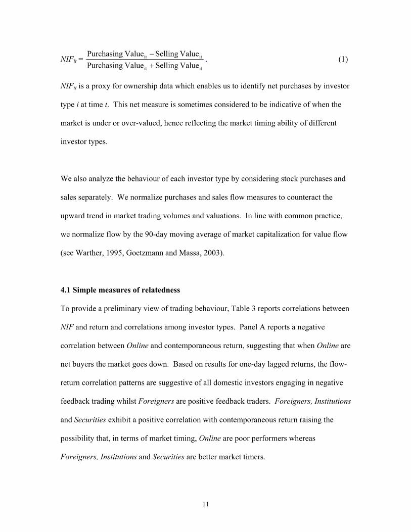
NIFit = itit

itit

Value SellingValue PurchasingValue SellingValue Purchasing

+−

. (1)

NIFit is a proxy for ownership data which enables us to identify net purchases by investor

type i at time t. This net measure is sometimes considered to be indicative of when the

market is under or over-valued, hence reflecting the market timing ability of different

investor types.

We also analyze the behaviour of each investor type by considering stock purchases and

sales separately. We normalize purchases and sales flow measures to counteract the

upward trend in market trading volumes and valuations. In line with common practice,

we normalize flow by the 90-day moving average of market capitalization for value flow

(see Warther, 1995, Goetzmann and Massa, 2003).

4.1 Simple measures of relatedness

To provide a preliminary view of trading behaviour, Table 3 reports correlations between

NIF and return and correlations among investor types. Panel A reports a negative

correlation between Online and contemporaneous return, suggesting that when Online are

net buyers the market goes down. Based on results for one-day lagged returns, the flow-

return correlation patterns are suggestive of all domestic investors engaging in negative

feedback trading whilst Foreigners are positive feedback traders. Foreigners, Institutions

and Securities exhibit a positive correlation with contemporaneous return raising the

possibility that, in terms of market timing, Online are poor performers whereas

Foreigners, Institutions and Securities are better market timers.

11

Panel B reports the relationship between investor types. Foreigners and all other investor

flows are negatively related. Combining this result with those of the flow return

correlations suggesting Foreigners are good market timers raises the specter that

domestic market participants, especially online investors, are liquidity providers to

foreigners. However, we regard these results as preliminary, and we conduct further tests

in which we control for other possible determinants in the sections below.

4.2 Detecting feedback trading

Feedback trading analysis based on correlations alone may give erroneous conclusions

due to possible multicollinearity. We use a bivariate vector autoregressive regression

(VAR) model to analyze whether online investors engage in feedback trading, following

Seasholes (2000) and Froot, O’Connell and Seasholes (2001). Econometrically, a VAR

model and its transformed representation constitute a useful tool which allows us to

effectively measure the impact of one variable on fluctuations of other variables in the

model.

The VAR model specification is:

t

p

jjtjt ZCZ ε+Φ+= ∑

=−

1 (2)

where Zt = C =

t

t

FR

F

R

αα

=Φ

pp

ppp

,2,2,2,1

,2,1,1,1

φφφφ

.

=

tF

tRt

,

,

εε

ε

Zt is a 2×1 matrix of return, Rt, and flow, Ft (Purchases, Sales or NIF) for day lag j, C is

the constant and εt is the 2×1 error matrix.

12

The VAR analysis constitutes estimates of reduced form equations with uniform sets of

lagged dependent variables from all equations as regressors. Using the Schwartz and

Alkaike criteria, we find that two lags of each variable are enough to capture the linear

interdependencies in the system. However, a five day lag is chosen to capture, and report

on, trading patterns over the preceding week.

Table 4 reports results from a bivariate VAR (5) model for all investors. Panel A, Part 1

reports the results for Online with Return as the dependent variable. All three flow types

(Purchases, Sales and NIF) and past returns fail to show any significant impact on

returns. This indicates that aggregate online flows do not move the market index. The

absence of a significant relationship between past returns and contemporaneous return

demonstrates that KSE is at least weak-form efficient. With Flow as a dependent variable

(Part 2), both market returns and past Online flows exhibit some significant relationship

to Online flows. For both Purchases and Sales flow measures, the market return impact

lasts up to four lags. It is interesting to observe that Purchases and Sales move in the

same direction. Yesterday’s return has a positive correlation with today’s flow for both

Purchases and Sales. Two day lagged returns are negatively correlated with both

Purchases and Sales. Hence, it is not surprising that we do not observe a significant

impact of market returns on NIF because it seems that Online as a group, do not share a

consensus on market movements and are likely to be just noise trading. It is therefore

hard to predict whether online investors are positive feedback traders (momentum

traders) or negative feedback traders (contrarians) at an aggregate level since there is no

distinct pattern of behaviour. The R2 value for Purchases and Sales is relatively high,

13

consistent with periods of boom and bust in trading levels, but low for NIF, consistent

with there being little information in the net opinion of online traders. Online exhibit

strong positive serial correlations in all three flows in that Online buys and sells tend to

lead other Online investors to buy and sell, demonstrating herding behaviour. This also

suggests that lagged online flow is a good indicator of contemporaneous flow.

Our results on Online flow’s relations with past returns differ from those of Jackson

(2003) who finds evidence of negative feedback trading by internet brokers driving the

overall observed relationships for a sample including full service brokers. Our results

also contrast with the findings on Finnish and US individual investors’ net flows by

Grinblatt and Keloharju (2001) and Odean (1998), respectively.

Similar to Online, results reported in Table 4 Panel B indicate that Foreigners past flows

and returns alike fail to explain changes in market return. However, past market returns

and flows do have some significant impacts for the three flows (Part 2). Unlike Online,

Foreigners do have a distinct pattern in their behaviour. Yesterday’s return has a

significant positive correlation on today’s Purchases but no significant impact for Sales,

a position confirmed by the significant positive impact on NIF. Similarly, returns posted

two days ago have no impact on today’s Purchases but are significantly positively

correlated to Sales, resulting in a significant negative relationship with NIF. This

illustrates that Foreigners as a group have more consensus (than Online) on the direction

of market movements. Part 2 also reports a significant sign reversal between one day

lagged returns and two day lagged returns for NIF flows. This may suggest that

14

Foreigners are profit seekers or bargain hunters who buy in up markets and sell the

following day, as it were to take profits. However, for a market that has been shown to

be at least weak form efficient, a more plausible interpretation is perhaps that foreigners,

as net sellers after market rises, are contrarians, and that gains posted in periods of

temporary price pressure reverse shortly afterwards due to the actions of other investors.

A significant positive coefficient is observed for Foreigners’ one day lagged flow and

current flow, which suggests that herding behaviour amongst Foreigners is also evident.

Table 4 Panel C (Part 1) reports results for Institutions with Return as the dependent

variable, and indicates that the coefficients on past returns are not significantly different

from zero. Unlike any other investors, Institutions two day lagged flows (NIF and Sales)

display a significant impact on returns suggesting the positive NIF impact on Return is

driven by negative Sales flow. In terms of results on Flow in Panel C (Part 2),

Institutions exhibit negative feedback trading. Yesterday’s return induces significantly

higher Sales and no clear impact on Purchases, thus leaving a negative NIF. The result

that Korean institutions are negative feedback traders contradicts findings for US

institutions which suggest positive feedback trading (Grinblatt, Titman and Wermers,

1995; Wermers, 1999; and Nofsinger and Sias, 1999) but portrays similarities to Japanese

institutions (Kim and Nofsinger, 2002). Since Institutions are net sellers and Foreigners

net buyers, it is possible that these two investor types interact. Positive serial correlation

is detected for up to a five day lag for Purchases and Sales but only up to a three day lag

15

for NIF. This result indicates possible herding behaviour by Institutions - yesterday’s

trading activity spurs other institutional investors to trade today.

Finally, Table 4 Panel D reports results for Securities. Analogous to Online, Foreigners,

and Institutions, past flows and returns for Securities display an insignificant impact on

Returns. However, both past returns and flows show some significant results for all three

flows. Securities exhibit significant net selling activity for one day lagged returns and net

buying activity for two day lagged returns which is the exact opposite of Foreigners

conduct, but in line with the behaviour of Institutions. This suggests that Securities, like

Institutions, interact with Foreigners. Positive serial correlation is evident for flows for

up to five days.

In summary, the R2 statistics reported for all investors in Table 4 indicate that past market

returns are an important variable in explaining flows whilst the explanatory power of past

flow measures on market returns is low. Past market returns do not have any significant

impact on current market returns. As well, significant positive serial correlations are

noted for Online, as with all other investor types, which suggest that there is significant

herding behaviour evident in the Korean market. All in all, online investors, like other

investor types, do not exhibit trading patterns that suggest particular skill in trading.

4.3 Is there information in flows?

Our analysis of the flow-return relationship is augmented in this section by further tests

of whether, beyond simply reacting to market returns, online investors’ flows contain any

16

information about market returns. The study by Cha and Lee (2001) conjectures that

flows may affect returns through either price pressure, or their effect on aggregate market

revisions of fundamentals about stock prices. Cha and Lee devise a method of

disentangling the price pressure and information effects of investor flows. Whilst it is

difficult to pinpoint the appropriate market fundamentals for purposes of our study, there

is reason to expect that, at the market level, dividends are important drivers of prices, as

too would be the risk premium. At the macroeconomic level interest rates and, for a

fairly open market like Korea, foreign exchange rates are further possible candidates.

We conduct the following regression analyses, loosely based on Cha and Lee (2001):

ξAxrateτAsprπDintDdivχFlowβRαRet3

1iit

3

1iitt ++++++= ∑∑

=−

=− ϖ , (3)

and

ρAxrateψAsprγDintνDdivFlowφRηlowF3

1iit

3

1iitt ++++++= ∑∑

=−

=− ϕ (4)

In the specifications, Flowt is measured by Purchases, Sales or NIF, Rt is market return

calculated by the natural logarithm of the difference between the level of the market

index on day t and day t-1; the market fundamentals are Ddiv, the dividend yield; Axrate,

the change in the foreign currency exchange rate (US dollar / Korean won); Aspr, the

spread, proxied by the difference between the 3-year government bond and 3-year

corporate bond rate; and Dint, the 90-day commercial paper rate. Since the frequency of

the data is daily and the market fundamentals do not fluctuate much on a daily basis, with

the exception of the foreign exchange rate, the variables are averaged over the past three

17

days. Short-term interest rates and dividend yields are differenced to meet stationarity

conditions.

Table 5 presents results of tests of Granger causality between flows and returns in the

presence of market fundamentals. The most interesting result in Panel A for Online is that

our specifications reject the null of no causality between net flows and returns whilst

failing to reject the null of causality in the opposite direction. The lack of causality from

flows to returns suggests the absence of any information in Online flows concerning

market returns. Strikingly, the significant impact (negative in sign) of two day lagged

returns on both Online Purchases and Sales followed by a positive reaction to returns the

following day, as reported in Panel A (Part 2), is consistent with the directionless nature

of online investor trades shown in Table 4. Online flows clearly contain information

about the following day’s flows, particularly in the case of disaggregated flows; however

only a low level of statistical significance applies to net flows lagged one day (again

emphasizing the absence of a clear trading strategy by online investors).

We contrast the flow-returns relations observed for Online with those for other investor

types. Generally net flows from Foreigners, Institutions and Securities (see Panels B

(Part 2), C (Part 2) and D (Part 2)) do not contain information about market returns in

the presence of market fundamentals. The exception is for Institutions flows lagged by

two days where we reject the null of causality from these flows to returns. This result

suggests domestic institutional investors are privy to some private information about

18

returns.12 This may be the signal used by Foreigners to purchase prudently, along with

Institutions themselves, the following day as their one day lagged purchases seem to

contain information about market returns even after incorporating market fundamentals

(possibly with Online and Securities being the providers of the necessary liquidity). The

non-online traders all appear to be influenced by past returns in their investment

strategies. The signs on the coefficients for one-day lagged returns suggest positive

feedback trading behaviour for Foreigners, and negative feedback trading by Institutions

and Securities. (See Panels B (Part 1), C (Part 1) and D (Part 1), respectively). The

difference in the behaviour of Foreigners compared to other non-online investors raises

questions about whether they act in a manner that exploits the trends observed for local

investors. However, this question is beyond the scope or our paper.

In possible vindication of online investors, it is interesting to note that all other investors’

flows are also subject to positive serial correlation. The levels of severity differ though –

for instance, for Institutions all lags of the various flow measures reveal strong positive

serial correlation; for Securities this phenomenon applies more significantly in the case of

disaggregated flows; and for Foreigners it is generally restricted to one lag of daily

flows. These results in part deflect the criticism of online investors to the extent that their

trading behaviour seems to be no more affected by past trading trends instead of market

fundamentals than other investor types.

12 Although we do not investigate this issue we note that the Korean corporate market is dominated by

cross-holding structures, Chaebols, of which the Institutions in our study often are part.

19

In summary, since for most investor types all three flows do not contain additional

information about returns over and above market fundamentals, it is likely that the price

pressure hypothesis does not hold. Flows from online investors, like those of other

investor types, simply respond to changes in market returns. In this regard, these findings

are consistent with results for US institutions (Cha and Lee, 2001), and imply that a

horizontal market demand curve for equities holds at an aggregate level. The presence of

strong positive serial correlation for all investors demonstrates that previous trading

activity by the same investor class has a significant impact on current flows. That this

phenomenon is shown to exist in the presence of market fundamentals emphasizes the

possible influence of herding on trading patterns amongst investors in the Korean stock

market at the expense of fundamental information.

4.4 Risk, uncertainty and market fundamentals as determinants of flows

According to finance theory investors’ decisions are based not only on expectations about

return but also on the uncertainty of those returns. What bearing does risk have on the

determinants of flow for online investors and how does this compare with other investor

types? In a classical CAPM model it is known that risk has negative utility effects on

investors and therefore a negative relationship with demand is expected. But if online

investors are unsophisticated and increase their comparative presence during periods of

market uncertainty, allegations about the detrimental effects of online trading are likely

justified. This is because it is usually speculators who enter the market and increase their

presence during periods of uncertainty, hoping to reap profits from volatility, driving

prices away from fundamentals (Goetzmann and Massa 2003). In the previous section

20

we investigated the relationship between flow and returns. In this section we examine

investors’ risk perceptions and behaviour and the role of risk in determining the volume

or demand for each investor type. We investigate the role of uncertainty in determining

flows using the following regression equation:

ttttt FInfVUncF εδγβα ++++= −1 (5)

where Ft denotes flow measurements as being Purchases, Sales, or NIF. InfVt is a vector

of “information variables” (or market fundamentals as explained in section 4.2), ε t is the

error term, and Unct represents the measure of uncertainty under consideration. The

specification is similar to that use by Goetzmann and Massa (2003).

Two proxies for uncertainty are considered. First, volatility is measured as the square of

the natural logarithm of return.13 Since anecdotal evidence suggests Korean investors are

mostly day-traders, intra-day volatility based on the Garman and Klass (1980) measure is

also used for robustness.14 Second, as an estimate of the dispersion of investor beliefs,

KOSPI 200 futures open interest, standardized by dividing daily open interest of KOSPI

13 Bae, Chan and Ng (2004) use this measure to capture the volatility in their study for all the emerging

markets which includes Korea.

14 Garman and Klass (1980) investigate the relative efficiency of various measures of volatility and identify

a volatility measure with the highest efficiency. In the so-called GK measure, written as

VAR(GK) is the variance using the

Garman-Klass (1980) method, LN denotes the natural logarithm, and High, Low, Open, Close are the high,

low, open, and closing prices of the day to determine the volatility.

,)]()(][1)2(2[)]()([5.0)( 22 CloseLNOpenLNLNLowLNHighLNGKVARt −−−−==∧σ

21

200 futures by the trading volume on KOSPI 200 futures contract on the same day, is

utilized.

The results, reported in Table 6 Panel A show that a strong positive relationship exists

between Unc (volatility) and disaggregated Online flows but not net flows (NIF). This

shows that volatility is an important contributor to Online flow even though the weak

relationship between volatility and NIF may demonstrate that Online increase their

presence in the market indiscriminately during volatile periods. Increasing both

Purchases and Sales during volatile periods may further increase volatility.15 Hence,

Online trading could be seen as speculation in the market during volatile periods,

possibly creating bubbles and a winner’s curse.16 Similar to our results for earlier tests, a

strong positive serial correlation persists for up to three days which may intensify the

creation of bubbles. One market fundamental, Ddiv, is significantly related to all three

flow measures. Remarkably, the positive relationship for NIF reported for Online in

Table 6 defies the trend of negative relations for all other investor types’ net flows. This

may indicate that online investors do take into consideration some fundamental

information, particularly easily accessible variables such as dividend yield, in

15 Perhaps this is the reason why online investors have been blamed for increasing volatility and

destabilizing the market. This is because during periods of higher volatility it is expected that speculators

would enter the market attracted by the possibility of higher gains, pushing prices away from the

fundamentals.

16 Speculative bubbles can also be manifestations of the ‘winners curse’. The winners curse is more likely

when there are more bidders and when the dispersion of opinions about the value of whatever is being

auctioned is greater.

22

determining their trade decisions, but they are still unable to process the information in a

manner that results in astute trading strategies. This supports the perception of online

investors as being naive market participants.

The other investor types, Foreigners, Institutions, and Securities all display a significant

positive relationship between volatility and Purchases and Sales in the presence of

market fundamentals but fail to show a significant relationship between volatility and

NIF. Clearly Online are not the only class of investors to increase Sales and Purchases

volume during volatile periods. This suggests that the market as a whole perceives

volatility as an opportunity to gain as suggested by Goetzmann and Massa (2003). For

non-online investors, the Dint market variable bears a significant positive influence on

disaggregated flows not borne out in net flow terms.

On the alternative volatility measure we adopt, the above results are qualitatively similar

for regressions incorporating the Garman and Klass intraday volatility computation.17

Another risk measure adopted in the model is dispersion of beliefs. Dispersion of beliefs

amongst investors is proxied for by the open interest of derivative contracts, the Korean

futures contracts. The relationship between level of dispersion and demand (Purchases

and Sales) is significantly negative for Online (see Table 6 Panel B) but, once again, the

relationship is insignificant for NIF. This indicates that during periods when there is

17 Results available from the authors on request.

23

disagreement about the future Online investors withdraw from the market

indiscriminately. The same results are evident for Institutions and Securities.

Foreigners, however, show a significant negative relationship for all three flows,

including NIF. The results indicate that Foreigners are more informed about the level of

dispersion of beliefs and withdraw from the market more discerningly. This is in line

with past research documenting that increases in the level of disagreement about the

future course of the market by sophisticated investors (those who use derivatives) induces

investors to be cautious (Goetzman and Massa, 2003). For Foreigners, clarity about the

future is an important determinant of the level of investor trading activity. The

interpretation of the rest of the explanatory variables remains unchanged for regressions

incorporating the dispersion of beliefs as a risk measure.

5. Trading performance

This section investigates whether each investor type’s trading is based on information

rather than cognitive biases. This is examined by analyzing post trading performance.

Specifically, more rigorous tests of market timing ability are carried out to examine the

extent to which trades affect prices in subsequent periods. Online investors have been

alleged to be poor performers or market timers and the evidence we have presented so far

appears to point in this direction. Hence this section shows, in comparison to other

investor types, whether online investors are indeed the losers in the market. Due to the

absence of portfolio holdings data, a direct estimate of investor group performance

cannot be implemented. However, following the work of Kamesaka, Nofsinger and

24

Kawakita (2003), this study utilizes daily purchase and sale flows to characterize the

market timing ability of these investor groups, which serves the purpose of proxying for

ownership or portfolio holdings when examining market returns after each trading day.

We firstly examine market performance after those days when investors conducted

particularly heavy buying or selling. We then estimate the cumulative return due to the

daily changes in investment flow and the subsequent market return for each investor

group.

5.1 Market timing ability

To examine whether the trading observed is motivated by information or cognitively

biased behaviour, the performance of investor groups after heavy buying and selling days

is measured. We conjecture that there is a stronger motivation behind heavy buying and

selling and it is on these days we expect to capture clearer evidence of information driven

or cognitively biased trading. After sorting each investor group’s data by level of NIF

into five equal sets, we class the highest positive NIF quintile as the buying days, and the

largest negative NIF the selling days. Daily, weekly and monthly market returns

following heavy buying and selling trading days are calculated. These give an indication

of market timing ability.

The results for performance after heavy buying and selling days in terms of value are

reported in Table 7. The imbalance of the buy and sell days is low for Online. Online,

on average, have NIFs of -0.037 and 0.054 during heavy sell and buy days, respectively.

The market rises after a day of heavy buying and selling by Online in a statistically

25

significant sense. But the market falls after a week and a month of heavy buying and

selling. This indicates that Online are relatively good at market timing for buys on a

daily basis and good market timing for sells on weekly and monthly basis. A comparison

of average trading imbalance between Online and the rest of traders on the KSE, reveals

that Online generally do not take extreme buy or sell positions. This may confirm that

Online are not well informed about the market and therefore do not have confidence to

take extreme trading positions.

Foreigners show relatively high buy and sell NIF imbalances. The market rises for up to

a week after heavy buying from Foreigners which shows Foreigners have good market

timing ability for buys. But after heavy sells from the Foreigners the market fails to

show significant declines, in fact there are significant increases. We conclude from this

asymmetry that Foreigners are therefore good at timing their buys but not their sells.

This result is similar to Online.

After a day of heavy buying and selling by Institutions, the market rises and declines,

albeit our results in this regard are without statistical significance. The t-statistics fail to

show any significance for post-trading performance for Institutions’ trades.

Securities on the other hand have the highest trading imbalance. The NIFs for heavy buy

and sell weeks are -0.395 and 0.330 respectively. The post-trading performance of

Securities is poor. The market rises after heavy sell days and the market declines after

heavy buy days. This poor performance persists for up to a month.

26

5.2 Cumulative performance

To investigate who are the ultimate winners and losers on the Korean Stock Exchange the

relative market timing ability of the investor groups based on the entire sample period,

rather than just heavy buying and selling days as in the previous section, is examined.

The performance measure used in this section was originally developed by Grinblatt and

Titman (1993) in their study based on the change in the portfolio holdings and later

modified by Karolyi (2002) and Kamesaka, Nofsinger and Kawakita (2003) by utilizing

net investment flows in the place of portfolio holdings. For a full description of the

derivation of the performance measure refer to Appendix 1.

The following empirical specification estimates the cumulative return due to the daily

changes in investment flow and following market returns:

∑+−

== −

−T

tt

1t1-t

1t1-t RSalesPurchaseSalesPurchase

( return Cumulative1

) (6)

where Purchases and Sales are raw values and Rt is the market return. Equation (6) is

estimated for each investor group in analyzing the performance over the entire sample

period.

Daily cumulative performance for the duration of sample period is graphed in Figure 2.

Consistent with performance based on heavy buy and sell days, cumulative performance

shows that Foreigners and Institutions attain the best returns. Online and Securities are

the losers but the extent of Securities’ losses is quite extreme compared to Online. Since

Securities have extreme positions (imbalances) which is a sign of herding (Nofsinger and

Sias, 1999), the inability to time the market would have devastating effects on their

27

performance at an aggregate level. On the other hand, because Online investors’ net

position is more or less balanced, their losses are probably mitigated.

5.3 Robustness tests

The results for Securities are surprising given that they are commonly presumed to be

more informed than other domestic traders. As such, we conduct a robustness check by

looking at weekly rather than daily performance. The weekly aggregation follows

convention as laid out in Lo and Wang (2000). The weekly cumulative performance is

graphed in Figure 3. The results are consistent for weekly as well as daily flows for

Foreigners, Institutions and Online but the opposite result to the daily returns is recorded

for Securities. Based on weekly returns Securities have positive returns. Foreigners are

a clear winner on the Korean stock exchange. Consistent with daily return results, Online

at an aggregate level are losers.

As a further robustness test, past, contemporaneous and lead return is regressed against

NIF for each investor type to assess whether they are good market timers and also to

investigate whether their flows affect future returns at daily and weekly frequencies. The

functional specification is:

εβα ++= ∑−

+

5

5iti tReNIF , (7)

where NIF is defined asSalesPurchasesSalesPurchases

+− for each investor type and lead/lag market

returns Ret is the return of KOSPI index.

28

Table 8 shows the relation between NIF for each investor type and lead/lag market

returns on daily and weekly basis, respectively. From observing daily past returns Online

investors are negative feedback traders whereas Foreigners are positive feedback traders

up to three day lag returns. Institutions and Securities also show negative feedback

trading at daily level. No significant results are present for weekly past returns.

The results from contemporaneous daily return show that Foreigners, Institutions and

Securities are good market timers, whereas Online display signs of naivety, increasing

their NIF on days when the market return is negative. In the results for weekly

contemporaneous return Foreigners continue to be winners, and Online remain as losers.

No significant results are evident for Institutions and Securities at weekly frequency.

To summarize our results on investor performance, Online show some superior market

timing ability during extreme buying positions up to a week. But looking at longer

horizons and taking into consideration all rather than just extreme cases, Online perform

poorly. This suggests that Online at an aggregate level are purely liquidity providers who

lose out to superior investors, although there exists some marginal online investors who

display superior performance as shown for extreme buying positions. Foreign investors,

in both general and extreme cases, record superior performance which supports the view

that foreigner trading is information driven (Seasholes, 2000, Froot, O’Connell and

Seasholes, 2001, Kamesaka, Nofsinger and Kawakita, 2003) and confirms that they are

the winners on the Korean stock exchange. However this result is contrary to Choe, Kho

29

and Stulz’s (2004) results based on data sampled during the Asian crisis for the Korean

market.

6. Summary and conclusions

In this study we utilize daily data from the highly active Korean stock market to

investigate the trading behaviour and performance of online investors. We compare our

online results with other investor types. Online investors do not exhibit distinct trading

patterns at an aggregate level and show signs of noise trading whereas foreigners,

institutions and securities companies exhibit some levels of intra-group consensus in the

direction of their trades in response to market movements. In the main, aggregated flows

from investors, with the exception of lagged local institutions’ trades, fail to explain

changes in the market index but the market index has a significant impact on investment

movements.

Positive serial correlation is persistent for all investors which raises concerns over the

results of investors’ actions. Serial correlation, when interpreted as herding, could push

prices away from fundamental values, destabilising the market (Lakonishok, Shleifer and

Vishny, 1992 and Wermers, 1999). This is more of a concern for online investors

relative to other investors since they constitute the vast majority of trading activity, in

both shares and value) on the KSE.

Results on the risk-volume relationship are similar for all groups – online investors join

other investor types in increasing their trading volumes indiscriminately during volatile

30

periods, suggesting that volatility is perceived as an opportunity. Our results based on the

dispersion of investor beliefs, proxied by open interest on the derivatives market, suggest

that only foreign investors discriminate between reductions in purchases and sales in

response to rising uncertainty.

Based on performance measures following periods of extreme imbalances in trading,

online investors, together foreign investors, record superior performance only at the

highest buying levels, but in aggregate their gains are likely neutralized by poor selling

positions. In the longer run, foreigners are the clear winners with online investors the

worst performers.

Our study may also have important policy implications. We find that online investors’

trading decisions are related to one variable, the dividend yield, amongst the proxies for

fundamental information that we adopt. Since this information is easily available even to

fairly naïve investors, one is driven to conjecture whether improvements in the way

online investors access quality information could instill more discipline in their trading

behaviour. As D’Avolio, Gildor and Shleifer (2001) have outlined, accurate information

must be available to be of use to investors. Because the trading community on the

Korean stock market mainly comprises online investors, the so-called unsophisticated

investors, there may be an incentive for information providers, who post better long term

gains, to discriminate against this source of cheap liquidity. Solutions need to be

carefully thought out, but the beginning point could involve greater efforts at investor

education.

31

With regards to the implications of this study for future research, it is important to note

that online investors dominate not only the equities market, but also the futures market.

As such, the behaviour of online traders and their performance in the derivatives market

is a potentially fruitful area for further research.

32

Appendix 1: Cumulative Performance Measure

The performance measure developed by Grinblatt and Titman (1993), based on changes

in portfolio holdings, captures the covariance between return on an asset and the change

in proportional holding of an asset as follows:

TRwwCOV tjtj

T

t

N

jtj /)( ,1,

1 1, −

= =∑ ∑ −= ,

where Rj is the return, wj is the weight of holding asset, N is the number of the assets and

T is the estimating sample period.

In this paper, we estimate this portfolio holding change measure for each investor i, using

modified conditions adopted by Karolyi (2002) and Kamesaka, Nofsinger and Kawakita

(2003).

The modified condition assumes that there are only two assets, one is the stock market

index and the other is the risk-free rate. The proxy for the daily or weekly market return

is calculated using the market index, the KOSPI index, and the daily risk free rate is

assumed to be zero. The modified measure is:

TRwwCOV tt

T

tt /)( 1

1−

=∑ −=

where Rt is the return on the market index during period t. Similar to Karolyi (2002) and

Kamesaka, Nofsinger and Kawakita (2003) we replace the change in portfolio weight

with net investment flows defined as SalesPurchasesSalesPurchases

+−

.

33

References

Bae, K., Chan, K., Ng, A., 2004. Investibility and return volatility. Journal of Financial Economics 71, 239-263. Barber, B., Odean, T., 2000. Trading is hazardous to your wealth: The common stock investment performance of individual investors. The Journal of Finance 55, 773-806. Barber, B., Odean, T., 2001. The internet and the investor. Journal of Economic Perspectives 15, 41-54. Barber, B., Odean, T., 2002. Online investors: Do the slow die first? Review of Financial Studies 15, 455-487. Brown, J., Goolsbee, A., 2002. Does the internet make markets more competitive? Evidence from the life insurance industry. Journal of Political Economy 110, 481-507. Byun, J., 2002. Online securities trading in Korea: Developments and trends. Working Paper, APEC Working Group on Electronic Financial Transactions Systems. Carhart, M. 1997. On persistence in mutual fund performance. The Journal of Finance 52, 57-82. Cha, H., Lee, B., 2001. The market demand curve for common stocks: Evidence from equity mutual fund flows. Journal of Financial and Quantitative Analysis 36, 195-220. Choe, H., Kho, B., Stulz, R., 1999. Do foreign investors destabilize stock markets? The Korean experience in 1997. Journal of Financial Economics 40, 31-62. Choe, H., Kho, B., Stulz, R., 2004. Do domestic investors have an edge? The trading experience of foreign investors in Korea. Working Paper , Ohio State University. Choi, J. J., Laibson, D., Metrick, A., 2002. How does the internet affect trading? Evidence from investor behavior in 401(k) plans. Journal of Financial Economics 64, 397-421. D’Avolio, G., Gildor, E., Schleifer, A., 2002. Technology, information production, and market efficiency. Economic Policy for the Information Economy, A Symposium Sponsored by the Federal Reserve Bank of Kansas City. Froot, K., O’Connell, P., Seasholes, M., 2001. The portfolio flows of international investors. Journal of Financial Economics 59, 151-193. Garman, M., Klass, M., 1980. On the estimation of security price volatilities from historical data. Journal of Business 53, 67-78.

34

Goetzmann, W., Massa, M., 2003. Index funds and stock market growth. Journal of Business 76, 1-28. Grinblatt, M., Keloharju, M., 2000. The investment behavior and performance of various investor-types: A study of Finland’s unique data set. Journal of Financial Economics 55, 43-67. Grinblatt, M., Titman, S., 1993. Performance measurement without benchmarks: An examination of mutual fund returns. Journal of Business 66, 47-68. Grinblatt, M., Titman, S., Wermers, R., 1995. Momentum investment strategies, portfolio performance, and herding: A study of mutual fund behavior. American Economic Review 85, 1088-1105. Jackson, A., 2003. The aggregate behaviour of individual investors. Working Paper, London School of Economics. Kamesaka, A., Nofsinger, J., Kawakita, H., 2003. Investment patterns and performance of investor groups in Japan. Pacific-Basin Finance Journal 11, 1-22. Karolyi, A., 2002. Did the Asian financial crisis scare foreign investors out of Japan? Pacific-Basin Finance Journal 10, 411-442. Kim, K., Nofsinger, J., 2002. Institutional herding, business groups, and economic regimes: Evidence from Japan. Working Paper, Washington State University. Kraus, A., Stoll, H., 1972a. Price impacts of block trading on the New York Stock Exchange. The Journal of Finance 27, 569-588. Kraus, A., Stoll, H., 1972b. Parallel trading by institutional investors. Journal of Financial and Quantitative Analysis 7, 2107-2138 Korea Securities Dealers Association., 2003. Securities Market in Korea 2003. Lakonishok, J., Shleifer, A., Vishny, R., 1992. The impact of institutional trading on stock prices. Journal of Financial Economics 32, 23-43. Lo, A., Wang, J., 2000. Trading volume: Definitions, data analysis, and implications of portfolio theory. Review of Financial Studies 13, 257-300. Madhavan, A., 2000. In search of liquidity in the internet era. Paper presented to the 9th annual financial markets conference of the Federal Reserve Bank of Atlanta. Nofsinger, J., Sias, R., 1999. Herding and feedback trading by institutional and individual investors. The Journal of Finance 54, 2263-2295.

35

Seasholes, M., 2000. Smart foreign traders in emerging markets. Working Paper, Harvard Business School. Warther, V., 1995. Aggregate mutual fund flows and security returns. Journal of Financial Economics 39, 209-235. Wermers, R., 1999. Mutual fund herding and the impact on stock prices. The Journal of Finance 54, 581-622.

36

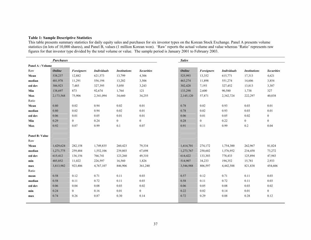
Table 1: Sample Descriptive Statistics This table presents summary statistics for daily equity sales and purchases for six investor types on the Korean Stock Exchange. Panel A presents volume statistics (in lots of 10,000 shares), and Panel B, values (1 million Korean won). ‘Raw’ reports the actual volume and value whereas ‘Ratio’ represents raw figures for that investor type divided by the total volume or value. The sample period is January 2001 to February 2003. Purchases Sales Panel A : Volume Raw Online Foreigners Individuals Institutions Securities Online Foreigners Individuals Institutions SecuritiesMean 538,237 12,882 621,573 13,799 4,306 525,993 13,352 615,771 17,313 4,621median 481,978 11,291 556,194 13,202 3,506 463,274 11,898 551,274 14,606 3,854std dev 306,923 7,485 327,395 5,050 3,243 302,428 7,193 327,452 13,813 3,387Min 138,697 873 92,674 1,764 121 133,298 2,600 90,580 1,738 327Max 2,173,568 75,906 2,341,094 34,660 34,255 2,145,120 57,871 2,342,724 222,297 40,038Ratio Mean 0.80 0.02 0.94 0.02 0.01 0.78 0.02 0.93 0.03 0.01median 0.80 0.02 0.94 0.02 0.01 0.78 0.02 0.93 0.03 0.01std dev 0.06 0.01 0.05 0.01 0.01 0.06 0.01 0.05 0.02 0Min 0.29 0 0.24 0 0 0.28 0 0.22 0 0Max 0.92 0.07 0.99 0.1 0.07 0.91 0.11 0.99 0.2 0.04 Panel B: Value Raw Mean 1,429,624 282,158 1,749,835 260,423 79,334 1,414,701 274,172 1,754,300 262,967 81,824median 1,271,775 259,484 1,552,106 239,803 67,698 1,273,767 250,602 1,576,952 234,458 73,272std dev 615,412 136,156 766,741 123,260 49,310 614,422 133,303 778,433 125,894 47,943min 485,852 11,022 226,597 16,560 1,826 514,907 34,233 194,352 15,781 2,933max 3,813,982 923,406 4,767,107 846,906 361,240 3,546,988 806,597 4,442,588 821,838 454,606Ratio mean 0.58 0.12 0.71 0.11 0.03 0.57 0.12 0.71 0.11 0.03median 0.58 0.11 0.72 0.11 0.03 0.58 0.11 0.72 0.11 0.03std dev 0.06 0.04 0.08 0.03 0.02 0.06 0.05 0.08 0.03 0.02min 0.24 0 0.16 0.01 0 0.22 0.02 0.14 0.01 0max 0.74 0.26 0.87 0.30 0.14 0.72 0.29 0.88 0.28 0.12

37

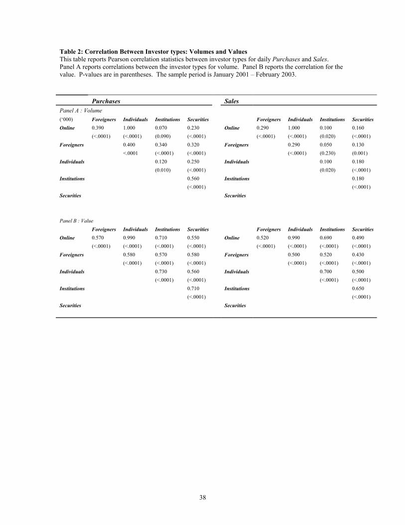
Table 2: Correlation Between Investor types: Volumes and Values This table reports Pearson correlation statistics between investor types for daily Purchases and Sales. Panel A reports correlations between the investor types for volume. Panel B reports the correlation for the value. P-values are in parentheses. The sample period is January 2001 – February 2003. Purchases Sales Panel A : Volume (‘000) Foreigners Individuals Institutions Securities Foreigners Individuals Institutions Securities Online 0.390 1.000 0.070 0.230 Online 0.290 1.000 0.100 0.160 (<.0001) (<.0001) (0.090) (<.0001) (<.0001) (<.0001) (0.020) (<.0001) Foreigners 0.400 0.340 0.320 Foreigners 0.290 0.050 0.130 <.0001 (<.0001) (<.0001) (<.0001) (0.230) (0.001) Individuals 0.120 0.250 Individuals 0.100 0.180 (0.010) (<.0001) (0.020) (<.0001) Institutions 0.560 Institutions 0.180 (<.0001) (<.0001) Securities Securities Panel B : Value Foreigners Individuals Institutions Securities Foreigners Individuals Institutions Securities Online 0.570 0.990 0.710 0.550 Online 0.520 0.990 0.690 0.490 (<.0001) (<.0001) (<.0001) (<.0001) (<.0001) (<.0001) (<.0001) (<.0001) Foreigners 0.580 0.570 0.580 Foreigners 0.500 0.520 0.430 (<.0001) (<.0001) (<.0001) (<.0001) (<.0001) (<.0001) Individuals 0.730 0.560 Individuals 0.700 0.500 (<.0001) (<.0001) (<.0001) (<.0001) Institutions 0.710 Institutions 0.650 (<.0001) (<.0001) Securities Securities

38

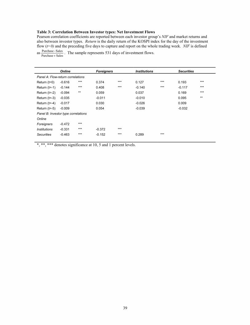
Table 3: Correlation Between Investor types: Net Investment Flows Pearson correlation coefficients are reported between each investor group’s NIF and market returns and also between investor types. Return is the daily return of the KOSPI index for the day of the investment flow (t=0) and the preceding five days to capture and report on the whole trading week. NIF is defined as

Sales PurchaseSales -Purchase

+. The sample represents 531 days of investment flows.

Online Foreigners Institutions Securities Panel A: Flow-return correlations Return (t=0) -0.616 *** 0.374 *** 0.127 *** 0.193 *** Return (t=-1) -0.144 *** 0.408 *** -0.140 *** -0.117 *** Return (t=-2) -0.094 ** 0.059 0.037 0.169 *** Return (t=-3) -0.035 -0.011 -0.010 0.095 ** Return (t=-4) -0.017 0.030 -0.026 0.009 Return (t=-5) -0.009 0.054 -0.039 -0.032 Panel B: Investor type correlations Online Foreigners -0.472 *** Institutions -0.331 *** -0.372 *** Securities -0.463 *** -0.152 *** 0.289 ***

*, **, *** denotes significance at 10, 5 and 1 percent levels.

39

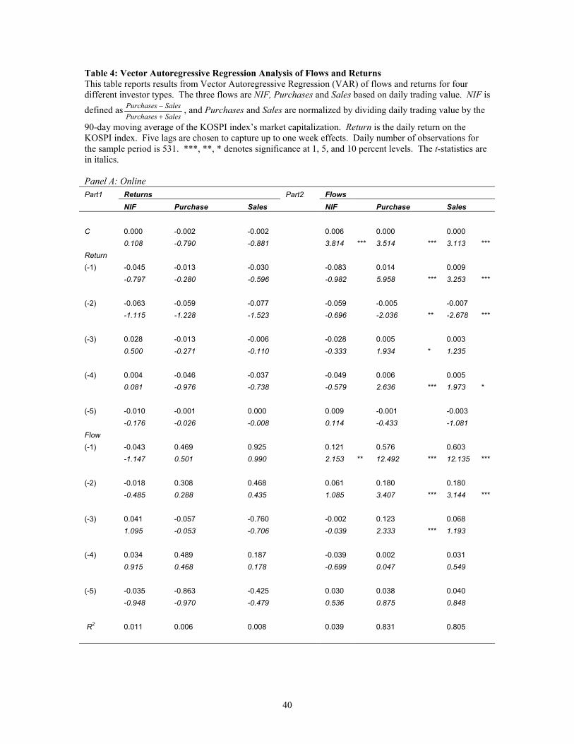
Table 4: Vector Autoregressive Regression Analysis of Flows and Returns This table reports results from Vector Autoregressive Regression (VAR) of flows and returns for four different investor types. The three flows are NIF, Purchases and Sales based on daily trading value. NIF is defined as

SalesPurchasesSalesPurchases

+− , and Purchases and Sales are normalized by dividing daily trading value by the

90-day moving average of the KOSPI index’s market capitalization. Return is the daily return on the KOSPI index. Five lags are chosen to capture up to one week effects. Daily number of observations for the sample period is 531. ***, **, * denotes significance at 1, 5, and 10 percent levels. The t-statistics are in italics. Panel A: Online Part1 Returns Part2 Flows NIF Purchase Sales NIF Purchase Sales C 0.000 -0.002 -0.002 0.006 0.000 0.000 0.108 -0.790 -0.881 3.814 *** 3.514 *** 3.113 *** Return (-1) -0.045 -0.013 -0.030 -0.083 0.014 0.009 -0.797 -0.280 -0.596 -0.982 5.958 *** 3.253 *** (-2) -0.063 -0.059 -0.077 -0.059 -0.005 -0.007 -1.115 -1.228 -1.523 -0.696 -2.036 ** -2.678 *** (-3) 0.028 -0.013 -0.006 -0.028 0.005 0.003 0.500 -0.271 -0.110 -0.333 1.934 * 1.235 (-4) 0.004 -0.046 -0.037 -0.049 0.006 0.005 0.081 -0.976 -0.738 -0.579 2.636 *** 1.973 * (-5) -0.010 -0.001 0.000 0.009 -0.001 -0.003 -0.176 -0.026 -0.008 0.114 -0.433 -1.081 Flow (-1) -0.043 0.469 0.925 0.121 0.576 0.603 -1.147 0.501 0.990 2.153 ** 12.492 *** 12.135 *** (-2) -0.018 0.308 0.468 0.061 0.180 0.180 -0.485 0.288 0.435 1.085 3.407 *** 3.144 *** (-3) 0.041 -0.057 -0.760 -0.002 0.123 0.068 1.095 -0.053 -0.706 -0.039 2.333 *** 1.193 (-4) 0.034 0.489 0.187 -0.039 0.002 0.031 0.915 0.468 0.178 -0.699 0.047 0.549 (-5) -0.035 -0.863 -0.425 0.030 0.038 0.040 -0.948 -0.970 -0.479 0.536 0.875 0.848 R2 0.011 0.006 0.008 0.039 0.831 0.805

40

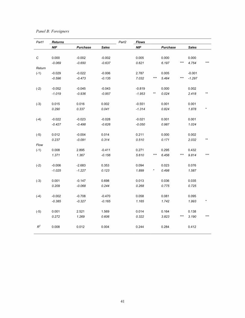
Panel B: Foreigners

Part1 Returns Part2 Flows NIF Purchase Sales NIF Purchase Sales C 0.000 -0.002 -0.002 0.005 0.000 0.000 -0.069 -0.650 -0.637 0.621 6.197 *** 4.754 *** Return (-1) -0.029 -0.022 -0.006 2.787 0.005 -0.001 -0.596 -0.473 -0.135 7.032 *** 5.464 *** -1.297 (-2) -0.052 -0.045 -0.043 -0.819 0.000 0.002 -1.019 -0.936 -0.957 -1.953 ** 0.024 2.418 ** (-3) 0.015 0.016 0.002 -0.551 0.001 0.001 0.290 0.337 0.041 -1.314 0.824 1.878 * (-4) -0.022 -0.023 -0.028 -0.021 0.001 0.001 -0.427 -0.498 -0.626 -0.050 0.987 1.024 (-5) 0.012 -0.004 0.014 0.211 0.000 0.002 0.237 -0.091 0.314 0.510 0.171 2.032 ** Flow (-1) 0.008 2.895 -0.411 0.271 0.295 0.432 1.371 1.367 -0.156 5.610 *** 6.456 *** 9.814 *** (-2) -0.006 -2.683 0.353 0.094 0.023 0.076 -1.025 -1.227 0.123 1.899 * 0.498 1.587 (-3) 0.001 -0.147 0.698 0.013 0.036 0.035 0.209 -0.068 0.244 0.268 0.775 0.725 (-4) -0.002 -0.708 -0.470 0.058 0.081 0.095 -0.385 -0.327 -0.165 1.165 1.742 1.993 * (-5) 0.001 2.521 1.569 0.014 0.164 0.138 0.272 1.269 0.606 0.322 3.823 *** 3.190 *** R2 0.008 0.012 0.004 0.244 0.284 0.412

41

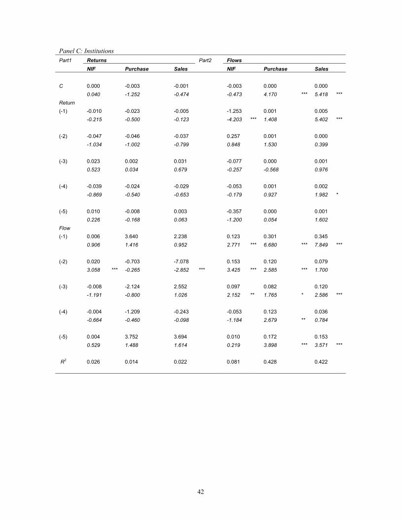
Panel C: Institutions Returns Flows Part1 Part2

Sales NIF Purchase Sales NIF Purchase

C 0.000 -0.003 -0.001 -0.003 0.000 0.000 0.040 -0.474 -0.473 4.170 *** 5.418 ***

(-1) -0.010 -0.023 -0.005 -1.253 0.001 0.005 -0.215 -0.500 -4.203 *** 1.408 5.402 *** (-2) -0.047 -0.046 -0.037 0.257 0.001 -1.034 -1.002 -0.799 0.848 0.399 (-3) 0.023 0.002 0.031 -0.077 0.000 0.001 0.523 0.034 0.679 -0.257 -0.568 0.976 (-4) -0.039 -0.024 -0.029 0.001 0.002

-1.252 Return

-0.123

0.000

1.530

-0.053

-0.869 -0.540 -0.653 -0.179 0.927 1.982 * (-5) 0.010 -0.008 0.003 -0.357 0.000 0.001 0.226 -0.168 0.063 -1.200 0.054 1.602 Flow (-1) 0.006 3.640 2.238 0.123 0.301 0.345 0.906 1.416 0.952 2.771 *** 6.680 *** 7.849 *** (-2) 0.020 -0.703 -7.078 0.153 0.120 0.079 3.058 *** -0.265 -2.852 *** 3.425 *** 2.585 *** 1.700 (-3) -0.008 -2.124 2.552 0.097 0.082 0.120 -1.191 -0.800 1.026 2.152 ** 1.765 * 2.586 *** (-4) -0.004 -1.209 -0.243 -0.053 0.123 0.036 -0.664 -0.460 -0.098 -1.184 2.679 ** 0.784 (-5) 0.004 3.752 3.694 0.010 0.172 0.153 0.529 1.488 1.614 0.219 3.898 *** 3.571 *** R2 0.026 0.014 0.022 0.081 0.428 0.422

42

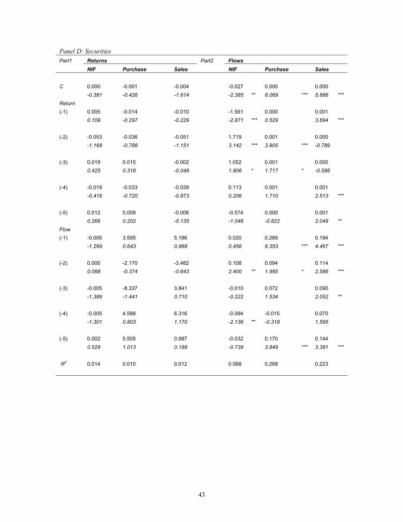
Panel D: Securities Part1 Returns Part2 Flows NIF Purchase Sales NIF Purchase Sales C 0.000 -0.001 -0.004 -0.027 0.000 0.000 -0.381 -0.426 -1.614 -2.385 ** 6.069 *** 5.886 *** Return (-1) 0.005 -0.014 -0.010 -1.561 0.000 0.001 0.109 -0.297 -0.229 -2.871 *** 0.529 3.694 *** (-2) -0.053 -0.036 -0.051 1.719 0.001 0.000 -1.168 -0.788 -1.151 3.142 *** 3.905 *** -0.789 (-3) 0.019 0.015 -0.002 1.052 0.001 0.000 0.425 0.316 -0.048 1.906 * 1.717 * -0.586 (-4) -0.019 -0.033 -0.039 0.113 0.001 0.001 -0.416 -0.720 -0.873 0.206 1.710 2.513 *** (-5) 0.012 0.009 -0.006 -0.574 0.000 0.001 0.266 0.202 -0.135 -1.046 -0.822 2.049 ** Flow (-1) -0.005 3.595 5.186 0.020 0.289 0.194 -1.269 0.643 0.968 0.456 6.353 *** 4.467 *** (-2) 0.000 -2.170 -3.482 0.108 0.094 0.114 0.088 -0.374 -0.643 2.400 ** 1.985 * 2.586 *** (-3) -0.005 -8.337 3.841 -0.010 0.072 0.090 -1.389 -1.441 0.710 -0.222 1.534 2.052 ** (-4) -0.005 4.588 6.316 -0.094 -0.015 0.070 -1.301 0.803 1.170 -2.136 ** -0.318 1.595 (-5) 0.002 5.505 0.987 -0.032 0.170 0.144 0.529 1.013 0.188 -0.739 3.849 *** 3.391 *** R2 0.014 0.010 0.012 0.068 0.268 0.223

43

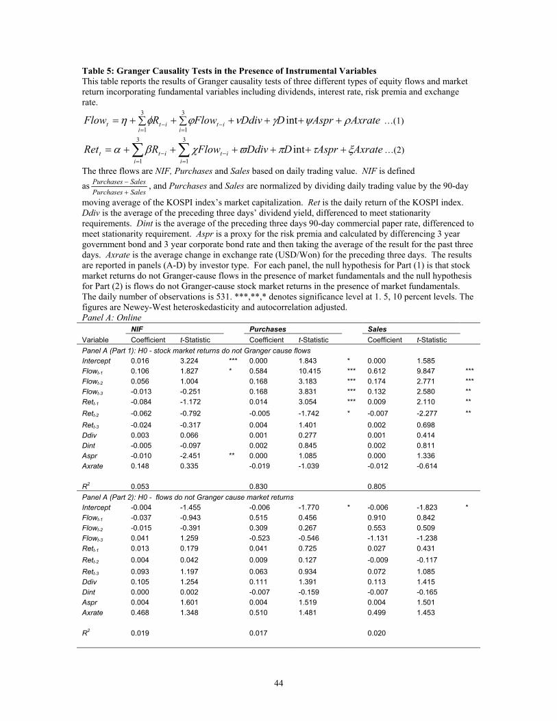
Table 5: Granger Causality Tests in the Presence of Instrumental Variables This table reports the results of Granger causality tests of three different types of equity flows and market return incorporating fundamental variables including dividends, interest rate, risk premia and exchange rate.

AxrateAsprDDdivFlowRFlowi

iti

itt ρψγνϕφη +++∑ ++∑+==

−=

− int3

1

3

1 …(1)

AxrateAsprDDdivFlowRReti

iti

itt ξτπϖχβα ++++++= ∑∑=

−=

− int3

1

3

1…(2)

The three flows are NIF, Purchases and Sales based on daily trading value. NIF is defined as

SalesPurchasesSalesPurchases

+− , and Purchases and Sales are normalized by dividing daily trading value by the 90-day

moving average of the KOSPI index’s market capitalization. Ret is the daily return of the KOSPI index. Ddiv is the average of the preceding three days’ dividend yield, differenced to meet stationarity requirements. Dint is the average of the preceding three days 90-day commercial paper rate, differenced to meet stationarity requirement. Aspr is a proxy for the risk premia and calculated by differencing 3 year government bond and 3 year corporate bond rate and then taking the average of the result for the past three days. Axrate is the average change in exchange rate (USD/Won) for the preceding three days. The results are reported in panels (A-D) by investor type. For each panel, the null hypothesis for Part (1) is that stock market returns do not Granger-cause flows in the presence of market fundamentals and the null hypothesis for Part (2) is flows do not Granger-cause stock market returns in the presence of market fundamentals. The daily number of observations is 531. ***,**,* denotes significance level at 1. 5, 10 percent levels. The figures are Newey-West heteroskedasticity and autocorrelation adjusted. Panel A: Online NIF Purchases Sales Variable Coefficient t-Statistic Coefficient t-Statistic Coefficient t-Statistic Panel A (Part 1): H0 - stock market returns do not Granger cause flows Intercept 0.016 3.224 *** 0.000 1.843 * 0.000 1.585 Flowt-1 0.106 1.827 * 0.584 10.415 *** 0.612 9.847 *** Flowt-2 0.056 1.004 0.168 3.183 *** 0.174 2.771 *** Flowt-3 -0.013 -0.251 0.168 3.831 *** 0.132 2.580 ** Rett-1 -0.084 -1.172 0.014 3.054 *** 0.009 2.110 ** Rett-2 -0.062 -0.792 -0.005 -1.742 * -0.007 -2.277 ** Rett-3 -0.024 -0.317 0.004 1.401 0.002 0.698 Ddiv 0.003 0.066 0.001 0.277 0.001 0.414 Dint -0.005 -0.097 0.002 0.845 0.002 0.811 Aspr -0.010 -2.451 ** 0.000 1.085 0.000 1.336 Axrate 0.148 0.335 -0.019 -1.039 -0.012 -0.614 R2 0.053 0.830 0.805 Panel A (Part 2): H0 - flows do not Granger cause market returns Intercept -0.004 -1.455 -0.006 -1.770 * -0.006 -1.823 * Flowt-1 -0.037 -0.943 0.515 0.456 0.910 0.842 Flowt-2 -0.015 -0.391 0.309 0.267 0.553 0.509 Flowt-3 0.041 1.259 -0.523 -0.546 -1.131 -1.238 Rett-1 0.013 0.179 0.041 0.725 0.027 0.431 Rett-2 0.004 0.042 0.009 0.127 -0.009 -0.117 Rett-3 0.093 1.197 0.063 0.934 0.072 1.085 Ddiv 0.105 1.254 0.111 1.391 0.113 1.415 Dint 0.000 0.002 -0.007 -0.159 -0.007 -0.165 Aspr 0.004 1.601 0.004 1.519 0.004 1.501 Axrate 0.468 1.348 0.510 1.481 0.499 1.453 R2 0.019 0.017 0.020

44

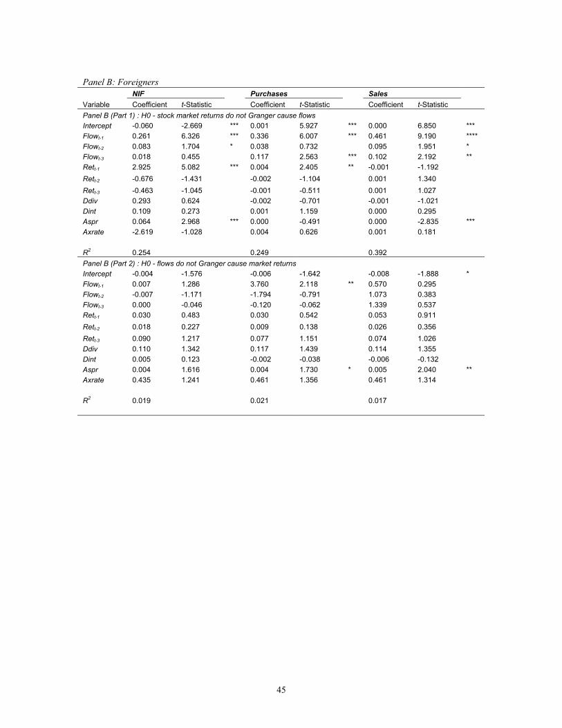
Panel B: Foreigners NIF Purchases Sales Variable Coefficient t-Statistic Coefficient t-Statistic Coefficient t-Statistic Panel B (Part 1) : H0 - stock market returns do not Granger cause flows Intercept -0.060 -2.669 *** 0.001 5.927 *** 0.000 6.850 *** Flowt-1 0.261 6.326 *** 0.336 6.007 *** 0.461 9.190 **** Flowt-2 0.083 1.704 * 0.038 0.732 0.095 1.951 * Flowt-3 0.018 0.455 0.117 2.563 *** 0.102 2.192 ** Rett-1 2.925 5.082 *** 0.004 2.405 ** -0.001 -1.192 Rett-2 -0.676 -1.431 -0.002 -1.104 0.001 1.340 Rett-3 -0.463 -1.045 -0.001 -0.511 0.001 1.027 Ddiv 0.293 0.624 -0.002 -0.701 -0.001 -1.021 Dint 0.109 0.273 0.001 1.159 0.000 0.295 Aspr 0.064 2.968 *** 0.000 -0.491 0.000 -2.835 *** Axrate -2.619 -1.028 0.004 0.626 0.001 0.181 R2 0.254 0.249 0.392 Panel B (Part 2) : H0 - flows do not Granger cause market returns Intercept -0.004 -1.576 -0.006 -1.642 -0.008 -1.888 * Flowt-1 0.007 1.286 3.760 2.118 ** 0.570 0.295 Flowt-2 -0.007 -1.171 -1.794 -0.791 1.073 0.383 Flowt-3 0.000 -0.046 -0.120 -0.062 1.339 0.537 Rett-1 0.030 0.483 0.030 0.542 0.053 0.911 Rett-2 0.018 0.227 0.009 0.138 0.026 0.356 Rett-3 0.090 1.217 0.077 1.151 0.074 1.026 Ddiv 0.110 1.342 0.117 1.439 0.114 1.355 Dint 0.005 0.123 -0.002 -0.038 -0.006 -0.132 Aspr 0.004 1.616 0.004 1.730 * 0.005 2.040 ** Axrate 0.435 1.241 0.461 1.356 0.461 1.314 R2 0.019 0.021 0.017

45

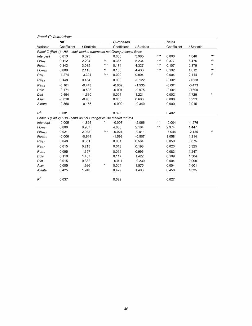
Panel C: Institutions NIF Purchases Sales Variable Coefficient t-Statistic Coefficient t-Statistic Coefficient t-Statistic Panel C (Part 1) : H0 - stock market returns do not Granger cause flows Intercept 0.013 0.623 0.000 3.985 *** 0.000 4.848 *** Flowt-1 0.112 2.294 ** 0.365 5.234 *** 0.377 6.476 *** Flowt-2 0.142 3.035 *** 0.174 4.327 *** 0.107 2.379 ** Flowt-3 0.088 2.115 ** 0.180 4.436 *** 0.192 4.612 *** Rett-1 -1.274 -3.304 *** 0.000 0.004 0.004 2.114 ** Rett-2 0.148 0.454 0.000 -0.122 -0.001 -0.638 Rett-3 -0.161 -0.443 -0.002 -1.535 -0.001 -0.473 Ddiv -0.171 -0.508 -0.001 -0.975 -0.001 -0.690 Dint -0.494 -1.630 0.001 1.221 0.002 1.729 * Aspr -0.018 -0.935 0.000 0.603 0.000 0.923 Axrate -0.368 -0.155 -0.002 -0.340 0.000 0.015 R2 0.081 0.393 0.402 Panel C (Part 2) : H0 - flows do not Granger cause market returns Intercept -0.005 -1.826 * -0.007 -2.066 ** -0.004 -1.276 Flowt-1 0.006 0.937 4.603 2.164 ** 2.974 1.447 Flowt-2 0.021 2.938 *** -0.024 -0.011 -6.044 -2.136 ** Flowt-3 -0.006 -0.914 -1.593 -0.807 3.058 1.214 Rett-1 0.048 0.851 0.031 0.564 0.050 0.875 Rett-2 0.015 0.215 0.013 0.198 0.023 0.325 Rett-3 0.095 1.357 0.066 0.996 0.083 1.247 Ddiv 0.118 1.437 0.117 1.422 0.109 1.304 Dint 0.015 0.382 -0.011 -0.239 0.004 0.090 Aspr 0.005 1.926 * 0.004 1.575 0.004 1.601 Axrate 0.425 1.240 0.479 1.403 0.458 1.335 R2 0.037 0.022 0.027

46

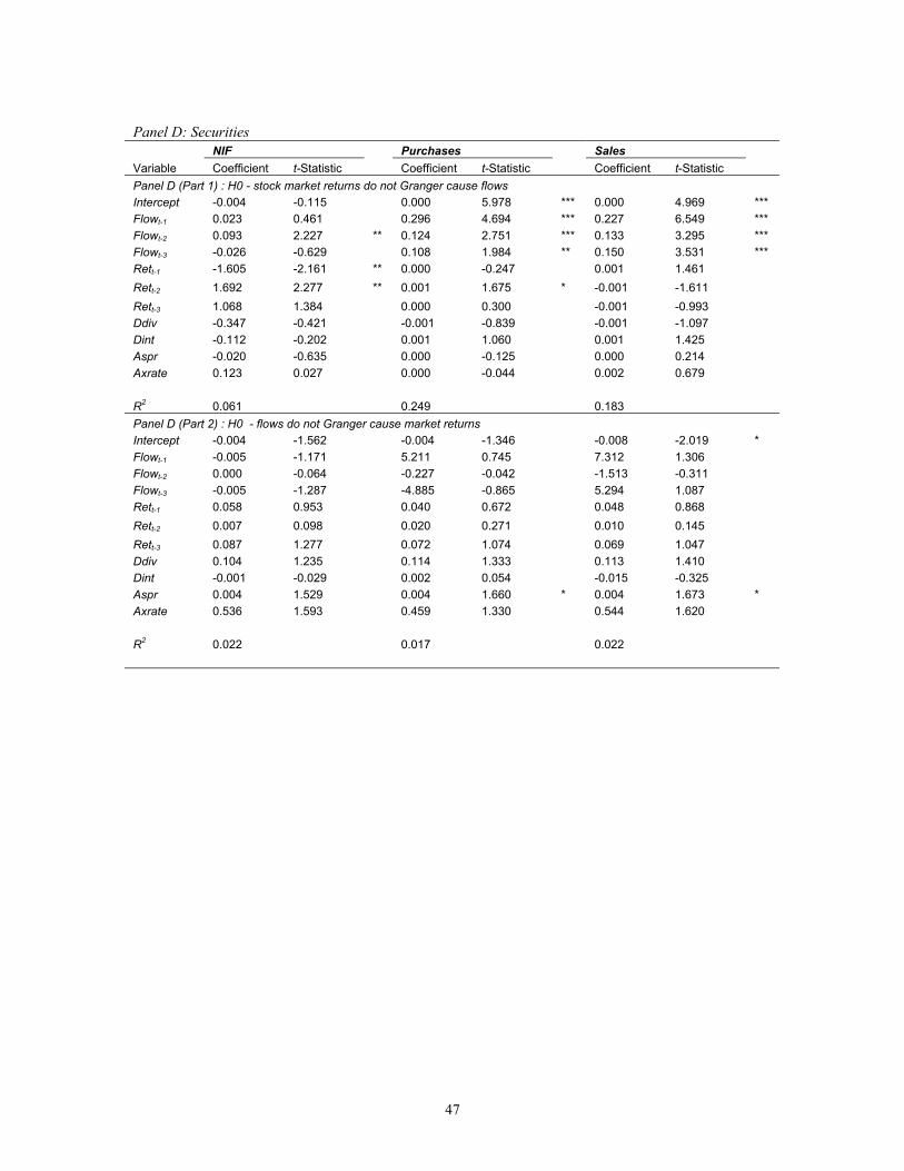
Panel D: Securities NIF Purchases Sales Variable Coefficient t-Statistic Coefficient t-Statistic Coefficient t-Statistic Panel D (Part 1) : H0 - stock market returns do not Granger cause flows Intercept -0.004 -0.115 0.000 5.978 *** 0.000 4.969 *** Flowt-1 0.023 0.461 0.296 4.694 *** 0.227 6.549 *** Flowt-2 0.093 2.227 ** 0.124 2.751 *** 0.133 3.295 *** Flowt-3 -0.026 -0.629 0.108 1.984 ** 0.150 3.531 *** Rett-1 -1.605 -2.161 ** 0.000 -0.247 0.001 1.461 Rett-2 1.692 2.277 ** 0.001 1.675 * -0.001 -1.611 Rett-3 1.068 1.384 0.000 0.300 -0.001 -0.993 Ddiv -0.347 -0.421 -0.001 -0.839 -0.001 -1.097 Dint -0.112 -0.202 0.001 1.060 0.001 1.425 Aspr -0.020 -0.635 0.000 -0.125 0.000 0.214 Axrate 0.123 0.027 0.000 -0.044 0.002 0.679 R2 0.061 0.249 0.183 Panel D (Part 2) : H0 - flows do not Granger cause market returns Intercept -0.004 -1.562 -0.004 -1.346 -0.008 -2.019 * Flowt-1 -0.005 -1.171 5.211 0.745 7.312 1.306 Flowt-2 0.000 -0.064 -0.227 -0.042 -1.513 -0.311 Flowt-3 -0.005 -1.287 -4.885 -0.865 5.294 1.087 Rett-1 0.058 0.953 0.040 0.672 0.048 0.868 Rett-2 0.007 0.098 0.020 0.271 0.010 0.145 Rett-3 0.087 1.277 0.072 1.074 0.069 1.047 Ddiv 0.104 1.235 0.114 1.333 0.113 1.410 Dint -0.001 -0.029 0.002 0.054 -0.015 -0.325 Aspr 0.004 1.529 0.004 1.660 * 0.004 1.673 * Axrate 0.536 1.593 0.459 1.330 0.544 1.620 R2 0.022 0.017 0.022

47

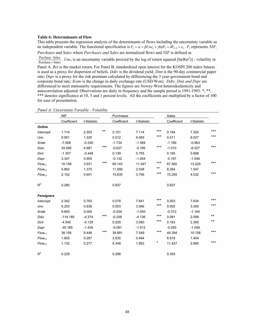
Table 6: Determinants of Flow This table presents the regression analysis of the determinants of flows including the uncertainty variable as an independent variable. The functional specification is ttttt FInfVUncF εδγβα ++++= −1 . Ft represents NIF, Purchases and Sales where Purchases and Sales are normalized flows and NIF is defined as

Sales PurchaseSales -Purchase

+. Unct is an uncertainty variable proxied by the log of return squared [ln(Ret2)] - volatility in

Panel A. Ret is the market return. For Panel B, standardized open interest for the KOSPI 200 index futures is used as a proxy for dispersion of beliefs. Ddiv is the dividend yield; Dint is the 90-day commercial paper rate; Dspr is a proxy for the risk premium calculated by differencing the 3 year-government bond and corporate bond rate; Xrate is the change in daily exchange rate (USD/Won). Ddiv, Dint and Dspr are differenced to meet stationarity requirements. The figures are Newey-West heteroskedasticity and autocorrelation adjusted. Observations are daily in frequency and the sample period is 1991-1993. *, **, *** denotes significance at 10, 5 and 1 percent levels. All the coefficients are multiplied by a factor of 100 for ease of presentation. Panel A: Uncertainty Variable - Volatility NIF Purchases Sales Coefficient t-Statistic Coefficient t-Statistic Coefficient t-Statistic Online Intercept 1.114 2.353 ** 0.151 7.114 *** 0.154 7.324 *** Unc 0.061 1.320 0.012 6.065 *** 0.011 6.027 *** Xrate -7.568 -0.240 -1.734 -1.584 -1.169 -0.963 Ddiv 34.595 4.681 *** -0.627 -5.185 *** -1.010 -6.527 *** Dint -1.357 -0.448 0.139 0.755 0.165 0.998 Dspr 3.347 0.905 -0.132 -1.054 -0.197 -1.546 Flowt-1 16.158 3.931 *** 65.143 11.547 *** 67.560 13.225 *** Flowt-2 5.862 1.375 11.590 2.038 ** 8.264 1.547 Flowt-3 2.152 0.601 15.635 3.756 *** 15.255 4.032 *** R2 0.280 0.837 0.837 Foreigners Intercept 2.342 0.763 0.078 7.641 *** 0.053 7.634 *** Unc 0.203 0.636 0.003 3.066 *** 0.002 3.300 *** Xrate 9.693 0.050 -0.534 -1.050 -0.312 -1.164 Ddiv -114.185 -4.374 *** -0.258 -4.136 *** 0.081 2.099 ** Dint -4.540 -0.129 0.205 3.060 *** 0.163 2.360 ** Dspr -35.185 -1.430 -0.091 -1.512 -0.055 -1.048 Flowt-1 38.156 9.448 *** 39.891 7.549 *** 49.394 10.158 *** Flowt-2 1.605 0.287 2.635 0.494 6.816 1.404 Flowt-3 1.132 0.277 8.348 1.952 * 11.427 2.685 *** R2 0.229 0.288 0.393

48

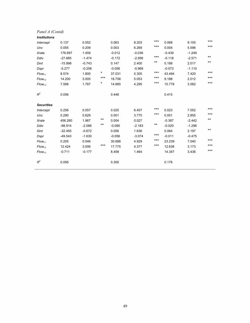
Panel A (Contd) Institutions Intercept 0.137 0.052 0.063 8.203 *** 0.068 9.105 *** Unc 0.055 0.209 0.003 6.269 *** 0.004 5.596 *** Xrate 176.697 1.459 -0.012 -0.036 -0.439 -1.249 Ddiv -27.685 -1.474 -0.172 -2.956 *** -0.118 -2.571 ** Dint -15.998 -0.743 0.147 2.400 ** 0.188 2.017 ** Dspr -5.277 -0.258 -0.056 -0.969 -0.073 -1.110 Flowt-1 8.574 1.800 * 37.031 5.305 *** 43.494 7.420 *** Flowt-2 14.200 3.005 *** 18.758 5.053 *** 9.188 2.012 *** Flowt-3 7.568 1.787 * 14.685 4.295 *** 15.778 3.582 *** R2 0.056 0.448 0.415 Securities Intercept 0.256 0.057 0.025 6.457 *** 0.023 7.052 *** Unc 0.290 0.629 0.001 3.770 *** 0.001 2.855 *** Xrate 456.260 1.967 ** 0.004 0.027 -0.387 -2.442 ** Ddiv -98.914 -2.066 ** -0.090 -2.183 ** -0.020 -1.296 Dint -32.455 -0.672 0.056 1.636 0.064 2.197 ** Dspr -49.543 -1.630 -0.056 -3.074 *** -0.011 -0.475 Flowt-1 0.205 0.046 30.688 4.929 *** 23.239 7.040 *** Flowt-2 12.424 3.006 *** 17.775 4.377 *** 12.638 3.173 *** Flowt-3 -0.711 -0.177 8.458 1.464 14.347 3.436 *** R2 0.056 0.300 0.176

49

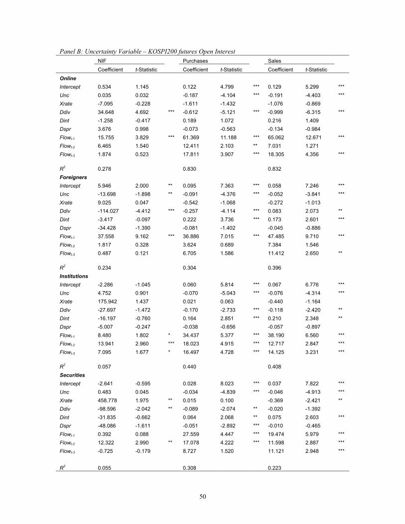
Panel B: Uncertainty Variable – KOSPI200 futures Open Interest NIF Purchases Sales Coefficient t-Statistic Coefficient t-Statistic Coefficient t-Statistic Online Intercept 0.534 1.145 0.122 4.799 *** 0.129 5.299 *** Unc 0.035 0.032 -0.187 -4.104 *** -0.191 -4.403 *** Xrate -7.095 -0.228 -1.611 -1.432 -1.076 -0.869 Ddiv 34.648 4.692 *** -0.612 -5.121 *** -0.999 -6.315 *** Dint -1.258 -0.417 0.189 1.072 0.216 1.409 Dspr 3.676 0.998 -0.073 -0.563 -0.134 -0.984 Flowt-1 15.755 3.829 *** 61.369 11.188 *** 65.062 12.671 *** Flowt-2 6.465 1.540 12.411 2.103 ** 7.031 1.271 Flowt-3 1.874 0.523 17.811 3.907 *** 18.305 4.356 *** R2 0.278 0.830 0.832 Foreigners Intercept 5.946 2.000 ** 0.095 7.363 *** 0.058 7.246 *** Unc -13.698 -1.898 ** -0.091 -4.376 *** -0.052 -3.841 *** Xrate 9.025 0.047 -0.542 -1.068 -0.272 -1.013 Ddiv -114.027 -4.412 *** -0.257 -4.114 *** 0.083 2.073 ** Dint -3.417 -0.097 0.222 3.736 *** 0.173 2.601 *** Dspr -34.428 -1.390 -0.081 -1.402 -0.045 -0.886 Flowt-1 37.558 9.162 *** 36.886 7.015 *** 47.485 9.710 *** Flowt-2 1.817 0.328 3.624 0.689 7.384 1.546 Flowt-3 0.487 0.121 6.705 1.586 11.412 2.650 ** R2 0.234 0.304 0.396 Institutions Intercept -2.286 -1.045 0.060 5.814 *** 0.067 6.776 *** Unc 4.752 0.901 -0.070 -5.043 *** -0.076 -4.314 *** Xrate 175.942 1.437 0.021 0.063 -0.440 -1.164 Ddiv -27.697 -1.472 -0.170 -2.733 *** -0.118 -2.420 ** Dint -16.197 -0.760 0.164 2.851 *** 0.210 2.348 ** Dspr -5.007 -0.247 -0.038 -0.656 -0.057 -0.897 Flowt-1 8.480 1.802 * 34.437 5.377 *** 38.190 6.560 *** Flowt-2 13.941 2.960 *** 18.023 4.915 *** 12.717 2.847 *** Flowt-3 7.095 1.677 * 16.497 4.728 *** 14.125 3.231 *** R2 0.057 0.440 0.408 Securities Intercept -2.641 -0.595 0.028 8.023 *** 0.037 7.822 *** Unc 0.483 0.045 -0.034 -4.839 *** -0.046 -4.913 *** Xrate 458.778 1.975 ** 0.015 0.100 -0.369 -2.421 ** Ddiv -98.596 -2.042 ** -0.089 -2.074 ** -0.020 -1.392 Dint -31.835 -0.662 0.064 2.068 ** 0.075 2.603 *** Dspr -48.086 -1.611 -0.051 -2.892 *** -0.010 -0.465 Flowt-1 0.392 0.088 27.559 4.447 *** 19.474 5.979 *** Flowt-2 12.322 2.990 ** 17.078 4.222 *** 11.598 2.887 *** Flowt-3 -0.725 -0.179 8.727 1.520 11.121 2.948 *** R2 0.055 0.308 0.223

50

Table 7: Market Performance after Heavy Buying and Selling This table reports the performance of different investor types at extreme ends of NIF. NIF is defined as

SalesPurchasesSalesPurchases

+− for each investor-group is sorted into

five equal sets. Periods of the highest positive NIF are designated the buying weeks, and those with the largest negative NIF the selling weeks. Each quintile of buy or sell weeks has 100 observations. One day, one week and one month returns are computed following the heavy buy or sell trading day. The mean NIF for heavy buying and selling days are reported in the table. The t-statistic tests the differences in mean between current and post trading returns and are reported in italic. NIF 1 day 1 week 1 month Sell Buy Sell Buy Sell Buy Sell Buy Online -0.037 0.054 0.004 0.001 -0.003 -0.001 -0.013 -0.009 7.644 ***

*** 0.185

-0.004 -0.005 0.229 0.452 -0.395 0.001 2.680 *** *

5.939 *** 4.989 *** 3.805 *** 3.608 *** 1.051Foreigners -0.260 0.306 0.000 0.003 0.007 0.000 0.007 0.010 3.872 *** 3.610 *** 3.915 2.618 *** 1.985 *Institutions -0.214 0.192 -0.002 0.002 0.007 -0.004 0.033 0.996 0.304 0.724Securities 0.330 -0.003 0.009 -0.009 0.011 0.002 3.119 *** 2.909 *** 3.314 ***

1.791 0.578

*, **, *** denotes significance at 10, 5 and 1 per cent level

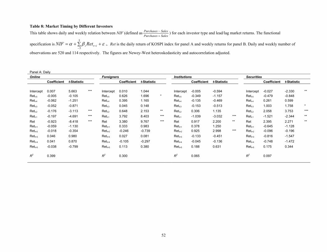
Table 8: Market Timing by Different Investors This table shows daily and weekly relation between NIF (defined as

SalesPurchasesSalesPurchases

+− ) for each investor type and lead/lag market returns. The functional

specification is .. Ret is the daily return of KOSPI index for panel A and weekly returns for panel B. Daily and weekly number of

observations are 520 and 114 respectively. The figures are Newey-West heteroskedasticity and autocorrelation adjusted.

εβα +∑+=−

+

5

5iti RetNIF

Panel A: Daily

Online Foreigners Institutions Securities Coefficient t-Statistic Coefficient t-Statistic Coefficient t-Statistic Coefficient t-Statistic

InterceptRet

5.663

-0.052 -0.871 Rett-3 0.045 0.148 Rett-3 -0.153 -0.176 *** Ret ** *** *** *** **

** 2.395 2.271 -0.645 -1.128 t+2 Ret Ret -0.816 -0.105 -0.297 Ret -0.045 -0.136 Ret 0.113 0.380 Ret 0.188 Ret

R

0.007 *** Intercept

0.010 1.044 Intercept

-0.005-0.349

-0.594 InterceptRet

-0.027 -2.330 **t-5 -0.005 -0.105 Rett-5 0.626 1.696 * Rett-5 -1.157 t-5 -0.479

0.261-0.848

Rett-4 -0.062 -1.251 Rett-4 0.395 1.165 Rett-4 -0.135 -0.469 Rett-4 0.599Rett-3 -0.513 Rett-3 1.003 1.758 *Rett-2 -3.113 t-2 0.648 2.153 Rett-2 0.306 1.135 Rett-2 2.058 3.753Rett-1 -0.197 -4.691 Rett-1 3.792 8.403 *** Rett-1 -1.039 -3.032 Rett-1 -1.521 -2.344Ret -0.923

-0.059-8.418 ***

Ret 3.380 9.767 ***

Ret 0.917

0.3782.200 Ret **

Rett+1 -1.130 Rett+1 0.333-0.246

0.983 Rett+1 1.2502.998

Rett+1

Rett+2 -0.018 -0.354 Rett+2 -0.739 Rett+2 0.925 *** Ret -0.096 -0.196Rett+3 0.046 0.980 t+3 0.027 0.081 Rett+3 -0.133 -0.451 t+3 -1.547Rett+4 0.041 0.870 Rett+4 t+4 Rett+4 -0.748 -1.472Rett+5 -0.038

-0.799

t+5 t+5 0.631

t+5 0.175

0.344

R2 0.399 2 0.300 R2 0.065 R2 0.097

52

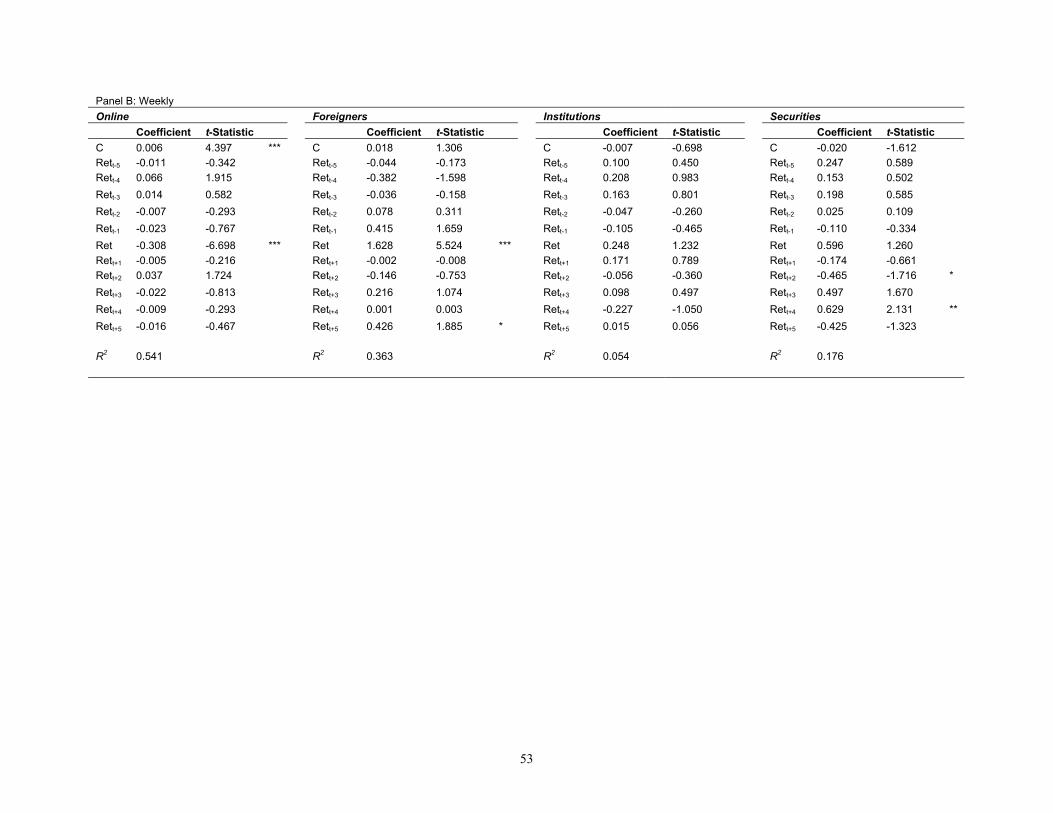
Panel B: Weekly Online Securities

Foreigners Institutions

Coefficient t-Statistic t-Statistic Coefficient t-Statistic Coefficient Coefficient t-Statistic C * 0.006 4.397 ** C 0.018 1.306 C -0.007 -0.698 C -0.020 -1.612 Rett-5 t-5

Ret -0.036 Ret 0.198 Ret Ret 0.025

Ret Ret *** 0.596

Ret t+2 -0.360 Ret *

Ret -0.022 Ret 0.216 Ret 0.001 0.003 -0.227 -0.016 -1.323

-0.011 -0.342 Rett-5 -0.044 -0.173 Ret 0.100 0.450 Rett-5 0.2470.153

0.589Rett-4 0.066 1.915 Rett-4 -0.382 -1.598 Rett-4 0.208 0.983 Rett-4 0.502

t-3 0.014 0.582 Rett-3 -0.158 t-3 0.163 0.801 Rett-3 0.585

t-2 -0.007 -0.293 Rett-2 0.078 0.311 t-2 -0.047 -0.260 Rett-2 0.109Rett-1 -0.023 -0.767 Rett-1 0.415 1.659 Rett-1 -0.105 -0.465 t-1 -0.110 -0.334RetRet

-0.308 -0.005

-6.698 ***

1.628 -0.002

5.524 Ret 0.248 1.232 Ret Ret

1.260t+1 -0.216

t+1 -0.008 Rett+1 0.171

-0.056 0.789 t+1 -0.174

-0.465 -0.661

Rett+2 0.037 1.724 Rett+2 -0.146 -0.753 Ret t+2 -1.716

t+3 -0.813 t+3 1.074 Rett+3 0.098 0.497 Rett+3 0.497 1.670Rett+4 -0.009 -0.293 t+4 Rett+4 -1.050 Rett+4 0.629 2.131 **Rett+5 -0.467 Rett+5 0.426 1.885 * Rett+5 0.015 0.056 Rett+5 -0.425

R2 0.541

R2 0.363 R2 0.054 R2 0.176

53

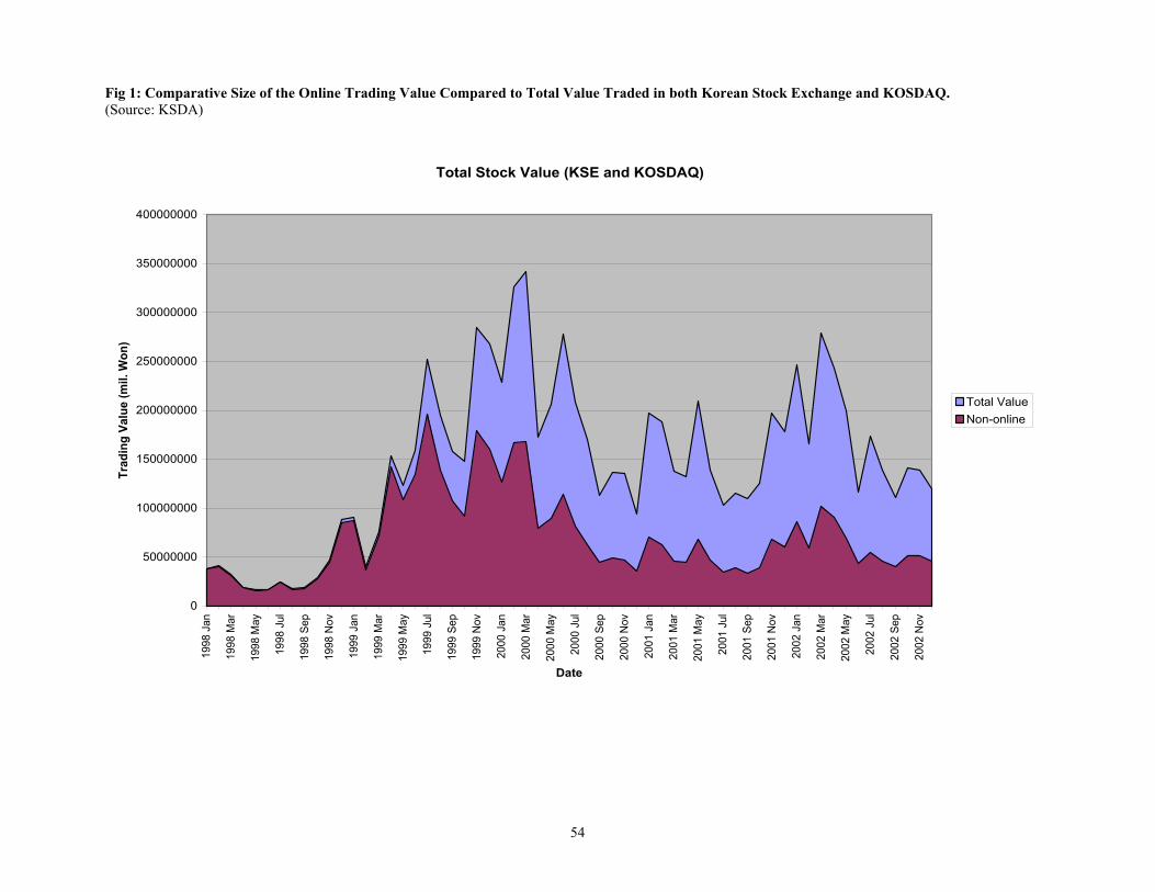
Fig 1: Comparative Size of the Online Trading Value Compared to Total Value Traded in both Korean Stock Exchange and KOSDAQ. (Source: KSDA)

Total Stock Value (KSE and KOSDAQ)

0

50000000

100000000

150000000

200000000

250000000

300000000

350000000

40000000019

98 J

an

1998

Mar

1998

May

1998

Jul

1998

Sep

1998

Nov

1999

Jan

1999

Mar

1999

May

1999

Jul

1999

Sep

1999

Nov

2000

Jan

2000

Mar

2000

May

2000

Jul

2000

Sep

2000

Nov

2001

Jan

2001

Mar

2001

May

2001

Jul

2001

Sep

2001

Nov

2002

Jan

2002

Mar

2002

May

2002

Jul

2002

Sep

2002

Nov

Date

Trad

ing

Valu

e (m

il. W

on)

Total ValueNon-online

54

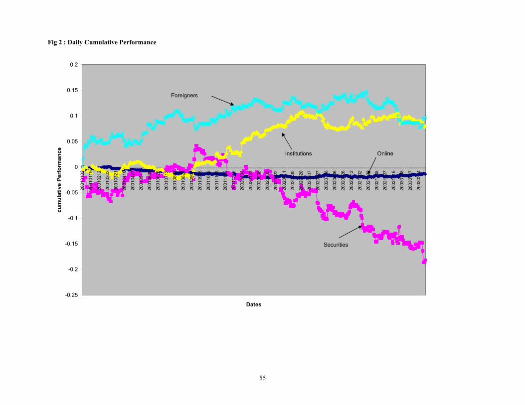
Fig 2 : Daily Cumulative Performance

-0.25

-0.2

-0.15

-0.1

-0.05

0

0.05

0.1

0.15

0.2

2001

0102

2001

0119

2001

0212

2001

0302

2001

0321

2001

0410

2001

0427

2001

0517

2001

0605

2001

0625

2001

0712

2001

0801

2001

0821

2001

0907

2001

0926

2001

1018

2001

1106

2001

1123

2001

1212

2002

0103

2002

0122

2002

0208

2002

0305

2002

0322

2002

0411

2002

0430

2002

0520

2002

0607

2002

0627

2002

0718

2002

0806

2002

0826

2002

0912

2002

1002

2002

1022

2002

1108

2002

1127

2002

1216

2003

0108

2003

0127

2003

0214

Dates

cum

ulat

ive

Perf

orm

ance

Foreigners

Institutions Online

Securities

55

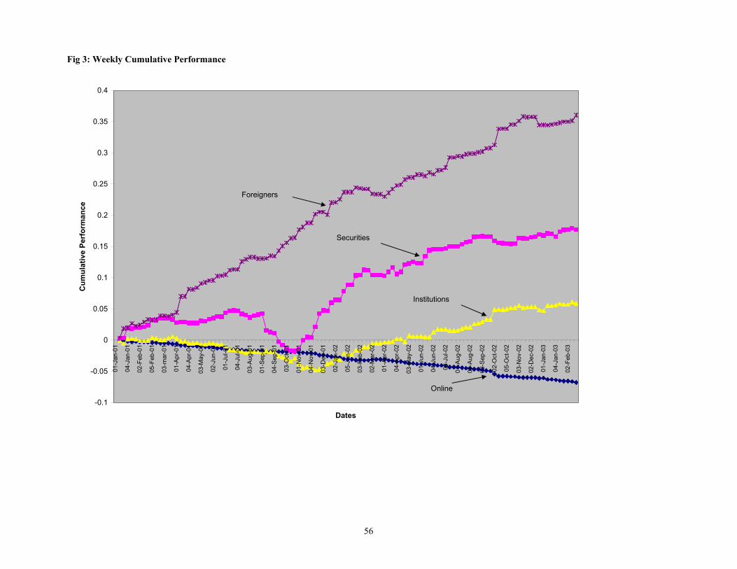
56

Fig 3: Weekly Cumulative Performance

-0.1

-0.05

0

0.05

0.1

0.15

0.2

0.25

0.3

0.35

0.4

01-J

an-0

1

04-J

an-0

1

02-F

eb-0

1

05-F

eb-0

1

03-m

ar-0

1

01-A

pr-0

1

04-A

pr-0

1

03-M

ay-0

1

02-J

un-0

1

01-J

ul-0

1

04-J

ul-0

1

03-A

ug-0

1

01-S

ep-0

1

04-S

ep-0

1

03-O

ct-0

1

01-N

ov-0

1

04-N

ov-0

1

03-D

ec-0

1

02-J

an-0

2

05-J

an-0

2

03-F

eb-0

2

02-M

ar-0

2

01-A

pr-0

2

04-A

pr-0

2

03-M

ay-0

2

01-J

un-0

2

04-J

un-0

2

03-J

ul-0

2

01-A

ug-0

2

04-A

ug-0

2

03-S

ep-0

2

02-O

ct-0

2

05-O

ct-0

2

03-N

ov-0

2

02-D

ec-0

2

01-J

an-0

3

04-J

an-0

3

02-F

eb-0

3

Dates

Cum

ulat

ive

Perf

orm

ance

Foreigners

Securities

Institutions

Online