Chapter 1 Simple Linear Regression

(part 4)

1 Analysis of Variance (ANOVA) approach to regressionanalysis

Recall the model again

Yi = β0 + β1Xi + εi, i = 1, ..., n

The observations can be written as

obs Y X

1 Y1 X1

2 Y2 X2...

......

n Yn Xn

The deviation of each Yi from the mean Y ,

Yi − Y

The fitted Yi = b0 + b1Xi, i = 1, ..., n are from the regression and determined by Xi.

Their mean is¯Y =

1n

n∑i=1

Yi = Y

Thus the deviation of Yi from its mean is

Yi − Y

The residuals ei = Yi − Yi, with mean is

e = 0 (why?)

Thus the deviation of ei from its mean is

ei = Yi−Yi

1

Write

Yi − Y︸ ︷︷ ︸Total deviation

= Yi − Y︸ ︷︷ ︸Deviation

due the regression

+ ei︸︷︷︸Deviation

due to the error

obs deviation of deviation of deviation ofYi Yi = b0 + b1Xi ei = Yi − Yi

1 Y1 − Y Y1 − Y e1 − e = e1

2 Y2 − Y Y2 − Y e2 − e = e2...

......

...n Yn − Y Yn − Y en − e = en

Sum of∑n

i=1(Yi − Y )2∑n

i=1(Yi − Y )2∑n

i=1 e2i

squares Total Sum Sum of Sum ofof squares squares due to squares of

regression error/residuals(SST) (SSR) (SSE)

We haven∑

i=1

(Yi − Y )2

︸ ︷︷ ︸SST

=n∑

i=1

(Yi − Y )2

︸ ︷︷ ︸SSR

+n∑

i=1

e2i

︸ ︷︷ ︸SSE

Proof:n∑

i=1

(Yi − Y )2 =n∑

i=1

(Yi − Y + Yi − Yi)2

=n∑

i=1

{(Yi − Y )2 + (Yi − Yi)2 + 2(Yi − Y )(Yi − Yi)}

= SSR + SSE + 2n∑

i=1

(Yi − Y )(Yi − Yi)

= SSR + SSE + 2n∑

i=1

(Yi − Y )ei

= SSR + SSE + 2n∑

i=1

(b0 + b1Xi − Y )ei

= SSR + SSE + 2b0

n∑i=1

ei + 2b1

n∑i=1

Xiei − 2Yn∑

i=1

ei

= SSR + SSE

It is also easy to check

SSR =n∑

i=1

(b0 + b1Xi − b0 − b1X)2 = b21

n∑i=1

(Xi − X)2 (1)

2

Breakdown of the degree of freedom

The degrees of freedom for SST is n − 1: noticing that

Y1 − Y , ....., Yn − Y

have one constraint∑n

i=1(Yi − Y ) = 0

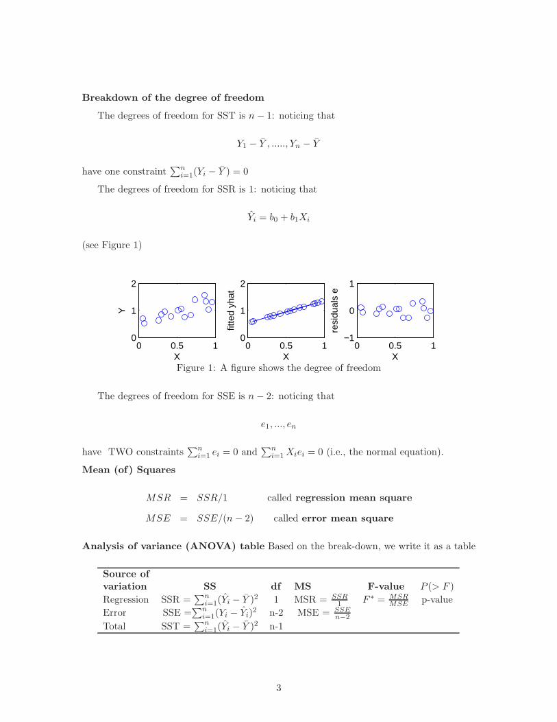
The degrees of freedom for SSR is 1: noticing that

Yi = b0 + b1Xi

(see Figure 1)

0 0.5 10

1

2

X

Y

0 0.5 10

1

2

X

fitte

d yh

at

0 0.5 1−1

0

1

X

resi

dual

s e

Figure 1: A figure shows the degree of freedom

The degrees of freedom for SSE is n − 2: noticing that

e1, ..., en

have TWO constraints∑n

i=1 ei = 0 and∑n

i=1 Xiei = 0 (i.e., the normal equation).

Mean (of) Squares

MSR = SSR/1 called regression mean square

MSE = SSE/(n − 2) called error mean square

Analysis of variance (ANOVA) table Based on the break-down, we write it as a table

Source ofvariation SS df MS F-value P (> F )Regression SSR =

∑ni=1(Yi − Y )2 1 MSR = SSR

1 F ∗ = MSRMSE p-value

Error SSE =∑n

i=1(Yi − Yi)2 n-2 MSE = SSEn−2

Total SST =∑n

i=1(Yi − Y )2 n-1

3

R command for the calculation

anova(object, ...)

where “object” is the output of a regression.

Expected Mean Squares

E(MSE) = σ2

and

E(MSR) = σ2 + β21

n∑i=1

(Xi − X)2

[Proof: the first equation was proved (where?). By (1), we have

E(MSR) = E(b1)2n∑

i=1

(Xi − X)2 = [V ar(b1) + (Eb1)2]n∑

i=1

(Xi − X)2

= [σ2∑n

i=1(Xi − X)2+ β2

1 ]n∑

i=1

(Xi − X)2 = σ2 + β21

n∑i=1

(Xi − X)2

]

2 F-test of H0 : β1 = 0

Consider the hypothesis test

H0 : β1 = 0, Ha : β1 �= 0.

Note that Yi = b0 + b1Xi and

SSR = b21

n∑i=1

(Xi − X)2

If b1 = 0 then SSR = 0 (why). Thus we can test β1 = 0 based on SSR. i.e. under H0, SSR

or MSR should be “small”.

We consider the F-statistic

F =MSR

MSE=

SSR/1SSE/(n − 2)

.

Under H0,

F ∼ F (1, n − 2)

For a given significant level α, our criterion is

4

If F ∗ ≤ F (1 − α, 1, n − 2) (i.e. indeed small), accept H0

If F ∗ > F (1 − α, 1, n − 2)(i.e. not small), reject H0

where F (1 − α, 1, n − 2) is the (1 − α) quantile of the F distribution.

We can also do the test based on the p-value = P (F > F ∗),

If p-value ≥ α, accept H0

If p-value < α, reject H0

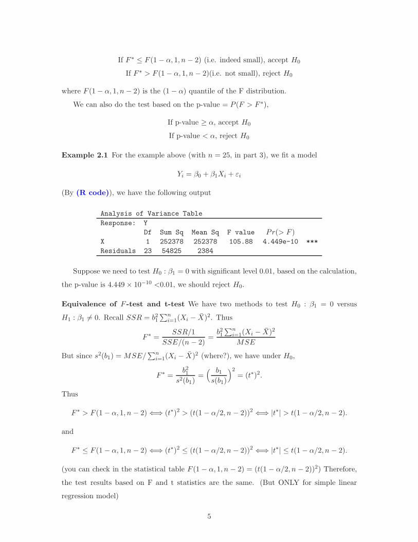
Example 2.1 For the example above (with n = 25, in part 3), we fit a model

Yi = β0 + β1Xi + εi

(By (R code)), we have the following output

Analysis of Variance TableResponse: Y

Df Sum Sq Mean Sq F value Pr(> F )X 1 252378 252378 105.88 4.449e-10 ***Residuals 23 54825 2384

Suppose we need to test H0 : β1 = 0 with significant level 0.01, based on the calculation,

the p-value is 4.449 × 10−10 <0.01, we should reject H0.

Equivalence of F -test and t-test We have two methods to test H0 : β1 = 0 versus

H1 : β1 �= 0. Recall SSR = b21

∑ni=1(Xi − X)2. Thus

F ∗ =SSR/1

SSE/(n − 2)=

b21

∑ni=1(Xi − X)2

MSE

But since s2(b1) = MSE/∑n

i=1(Xi − X)2 (where?), we have under H0,

F ∗ =b21

s2(b1)=

( b1

s(b1)

)2= (t∗)2.

Thus

F ∗ > F (1 − α, 1, n − 2) ⇐⇒ (t∗)2 > (t(1 − α/2, n − 2))2 ⇐⇒ |t∗| > t(1 − α/2, n − 2).

and

F ∗ ≤ F (1 − α, 1, n − 2) ⇐⇒ (t∗)2 ≤ (t(1 − α/2, n − 2))2 ⇐⇒ |t∗| ≤ t(1 − α/2, n − 2).

(you can check in the statistical table F (1 − α, 1, n − 2) = (t(1 − α/2, n − 2))2) Therefore,

the test results based on F and t statistics are the same. (But ONLY for simple linear

regression model)

5

3 General linear test approach

To test whether H0 : β1 = 0, we can do it by comparing two models

Full model : Yi = β0 + β1Xi + εi

and

Reduced model : Yi = β0 + εi

Denote the SSR of the FULL and REDUCED models by SSR(F ) and SSR(R) respec-

tively (and SSE(R), SSR(F)). We have immediately

SSR(F ) ≥ SSR(R)

or

SSE(F ) ≤ SSE(R).

A question: when does the equality hold?

Note that if H0 : β1 = 0 holds, then

SSE(R) − SSE(F )SSE(F )

should be small

Considering the degree of freedoms, define

F =(SSE(R) − SSE(F ))/(dfR − dfF )

SSE(F )/dfFshould be small

where dfR and dfF indicate the degrees of freedom of SSE(R) and SSE(F ) respectively.

Under H0 : β1 = 0, it is proved that

F ∼ F (dfR − dfF , dfF )

Suppose we get the F value as F ∗, then

If F ∗ ≤ F (1 − α, dfR − dfF , dfF ), accept H0

If F ∗ > F (1 − α, dfR − dfF , dfF ), reject H0

Similarly, based on the p-value = P (F > F ∗),

If p-value ≥ α, accept H0

If p-value < α, reject H0

6

4 Descriptive measures of linear association between X andY

It follows from

SST = SSR + SSE

that

1 =SSR

SST+

SSE

SST

where

• SSRSST is the proportion of Total sum of squares that can be explained/predicted by the

predictor X

• SSESST is the proportion of Total sum of squares that caused by the random effect.

A “good” model should have large

R2 =SSR

SST= 1 − SSE

SST

R2 is called R−square, or coefficient of determination

Some facts about R2 for simple linear regression model

1. 0 ≤ R2 ≤ 1.

2. if R2 = 0, then b1 = 0 (because SSR = b21

∑ni=1(Xi − X)2)

3. if R2 = 1, then Yi = b0 + b1Xi (why?)

4. the correlation coefficient between

rX,Y = ±√

R2

[Proof:

R2 =SSR

SST=

b21

∑ni=1(Xi − X)2∑n

i=1(Yi − Y )2= r2

XY

5. R2 only indicates the fitness in the observed range/scope. We need to be careful if we

make prediction outside the range.

6. R2 only indicates the ”linear relationships”. R2 = 0 does not mean X and Y have no

nonlinear association.

7

5 Considerations in Applying regression analysis

1. In prediction a new case, we need to ensure the model is applicable to the new case.

2. Sometimes we need to predict X, and thus predict Y . As a consequence, the prediction

accuracy also depends on the prediction of X

3. The range of X for the model. If a new case X is far from the range, in the prediction,

we need be careful

4. β1 �= 0 only indicates the correlation relationship, but not a cause-and-effect relation

(causality).

5. Even if β1 = 0 can be concluded, we cannot say Y has no relationship/association

with X. We can only say there is no LINEAR relationship/association between X

and Y .

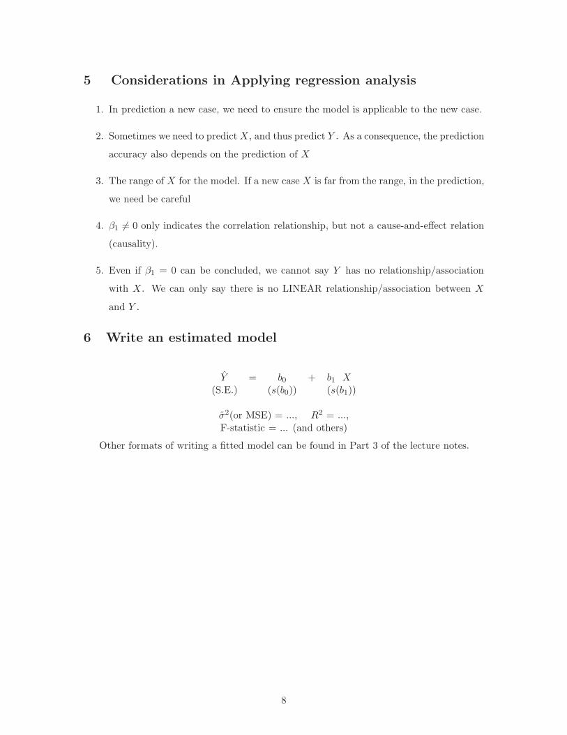
6 Write an estimated model

Y = b0 + b1 X(S.E.) (s(b0)) (s(b1))

σ2(or MSE) = ..., R2 = ...,F-statistic = ... (and others)

Other formats of writing a fitted model can be found in Part 3 of the lecture notes.

8