An Introduction to Generalized Linear Models (third edition, 2008) by Annette Dobson &

Adrian Barnett Outline of solutions for selected exercises

CHAPTER 1

1.1 1

2

5 23 2~ ,

2 2 53WW

⎡ ⎤⎛ ⎞ ⎛ ⎞ ⎛ ⎞⎢ ⎥⎜ ⎟ ⎜ ⎟ ⎜ ⎟⎝ ⎠ ⎝ ⎠⎝ ⎠ ⎣ ⎦

N .

1.2 (a) 2 (1)χ , by property 1 for the chi-squared distribution (page 7).

(b) 2

T 2 221

3 ~ (2)χ , by property 3. 2

YY −⎛ ⎞= + ⎜ ⎟⎝ ⎠

y y

(c) , by property 6. 2 2 21 2

-1 4 ~ (2, 9 / 4)T Y Y / χ+y V y =

1.3 (a) ( ) ( ) ( ) ( )( ) ( )2 2-1 2~ (2)Q Y χ . This

can be verified by considering

1 1 1 2 21 9 2 2 2 3 4 335

T Y Y Y⎡ ⎤= = − − − − + −⎣ ⎦y -μ V y -μ

( )1 22U Υ Υ+ and 1

2 153= − ( )1 2

13 2 12V −

and showing that U and V are independent, identically distributed random

variables with the distribution N(0, 1) and that 2 2Q U V

2 21Υ Υ= +

.= +

(b) ( )-1 2 2 22 1 1 2 2

1 9 2 4 ~ (2,12 / 735

T )YY Y χ= = − +y V yQ Y By property 6.

This can be verified by showing that 2

2

2

2 37

Q U V⎛

= + +⎜⎜ ⎟⎝ ⎠

⎞⎟ , so by property 4

22 3 12

77λ

⎛ ⎞= =⎜ ⎟⎜ ⎟⎝ ⎠

.

1.4 (a) ( )2~ , /Y N nμ σ

(c) and (d) follow from results on p.10, ( ) ( )2 2 21 / ~ 1n S nσ χ− − .

(e) If ( ) ( ) ( )2 1n − 2 2 2and~ 0,1 1 / ~/

YZ N U n Snμ σ χ

σ−

= = −

then ( )

( )1/ 22~ 1 .

/ / 1

Y Z t nS n U n

μ−= −⎡ ⎤−⎣ ⎦

1.5 (b) and (c) ( )ˆ log yβ =

1

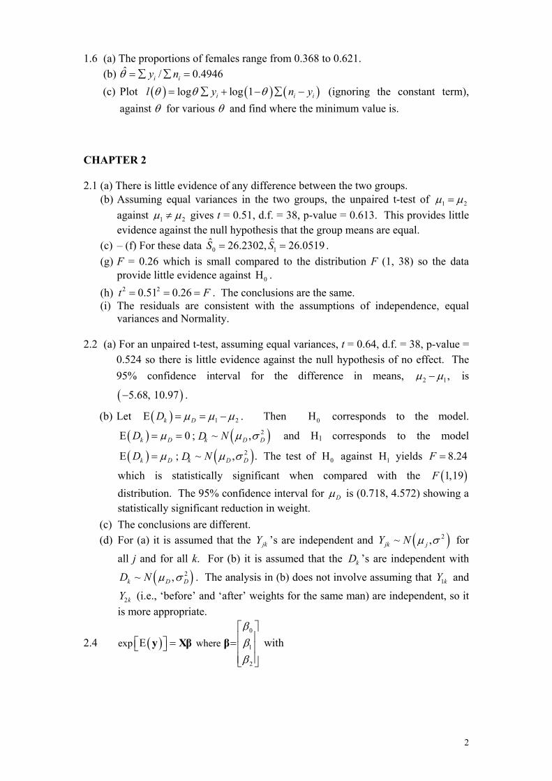
1.6 (a) The proportions of females range from 0.368 to 0.621. (b) ˆ / 0.4946i iy nθ = ∑ ∑ =

(c) Plot ( ) ( ) ( )log log 1il y nθ θ θ= ∑ + − ∑ −i iy (ignoring the constant term), against θ for various θ and find where the minimum value is.

CHAPTER 2 2.1 (a) There is little evidence of any difference between the two groups.

(b) Assuming equal variances in the two groups, the unpaired t-test of 1 2μ μ= against 1 2μ μ≠ gives t = 0.51, d.f. = 38, p-value = 0.613. This provides little evidence against the null hypothesis that the group means are equal.

(c) – (f) For these data . 0 1ˆ ˆ26.2302, 26.0519S S= =

(g) F = 0.26 which is small compared to the distribution F (1, 38) so the data provide little evidence against 0H .

(h) F . The conclusions are the same. 2 20.51 0.26t = = =(i) The residuals are consistent with the assumptions of independence, equal

variances and Normality.

2.2 (a) For an unpaired t-test, assuming equal variances, t = 0.64, d.f. = 38, p-value = 0.524 so there is little evidence against the null hypothesis of no effect. The 95% confidence interval for the difference in means, 2 1,μ μ− is

. ( )5.68, 10.97−

(b) Let 2( ) 1E k DD μ μ μ= = −

( ). Then 0H corresponds to the model.

( )2,D DE 0 ;k D kD D ~ Nμ μ σ and H1 corresponds to the model

)2, .Dμ σ The test of 0H against 1H yields 8.24F =

which is statistically significant when compared with the ( )1,19F distribution. The 95% confidence interval for

= =

( ) (E ; ~k D k DD NDμ=

Dμ is (0.718, 4.572) showing a statistically significant reduction in weight.

(c) The conclusions are different. (d) For (a) it is assumed that the jkY ’s are independent and ( )2~ ,jk jY N μ σ for

all j and for all k. For (b) it is assumed that the kD ’s are independent with

)2D(~ ,k DD N μ σ . The analysis in (b) does not involve assuming that 1kY and

2kY (i.e., ‘before’ and ‘after’ weights for the same man) are independent, so it is more appropriate.

2.4 ( )exp whereEβββ

0

1

2

⎡ ⎤⎢ ⎥= =⎡ ⎤⎣ ⎦ ⎢ ⎥⎢ ⎥⎣ ⎦

y Xβ β with

2

and X = .

3.154.856.507.208.25

16.50

⎡ ⎤⎢ ⎥⎢ ⎥⎢ ⎥

= ⎢⎢ ⎥⎢ ⎥⎢ ⎥⎣ ⎦

y ⎥

1 1.0 1.001 1.2 1.441 1.4 1.961 1.6 2.561 1.8 3.241 2.0 4.00

⎡ ⎤⎢ ⎥⎢ ⎥⎢ ⎥⎢ ⎥⎢ ⎥⎢ ⎥⎢ ⎥⎢ ⎥⎣ ⎦

2.5 where ( )E =y Xβ

1 1 1 01 1 0 11 1 1 11 1 1 01 1 0 11 1 1 1

⎡ ⎤⎢ ⎥⎢ ⎥⎢ ⎥− −

= ⎢ −⎢ ⎥⎢ ⎥−⎢ ⎥

⎥

− − −⎣ ⎦

X and 1

1

2

μαββ

⎡ ⎤⎢ ⎥⎢ ⎥=⎢ ⎥⎢ ⎥⎣ ⎦

β .

CHAPTER 3 3.1 (a) Response: = weight – continuous scale, possibly Normally distributed; iY

Explanatory variables: 1ix = age, 2ix = sex (indicator variable), 3ix = height,

4ix = mean daily food intake, and 5ix =mean daily energy expenditure;

( ) ( )20 1 1 2 2 3 3 4 4 5 5E ;i i i i i i i i iY x x x x x Y N~ , .μ β β β β β β μ σ= = + + + + + .

(b) Response: Y = number of mice infected in each group of 20n = mice;

Explanatory variables: 1,...,i 5ix x as indicator variables for exposure levels; ~iY binomial ( , in )π because ‘infection’ is a binary outcome (but the

plausibility of the assumption of independence of infection for mice depends on the experimental conditions); ( ) 0 1 1 2 2 3 3 4 4 5i i i i ig x x x xπ β β β β β β= + + + + + 5ix with the kβ ’s subject to a

corner point or sum-to-zero constraint.

(c) Response: iY = number of trips per week; Explanatory variables: 1ix = number of people in the household, 2ix = household income, 3ix = distance to supermarket;

~iY Poisson ( )iλ is a simple model for count data with

0 1 1 2 2 3log i i i 3ix x xλ β β β β= + + + .

3.2 ( ) ( ) ( ) ( ) ( ) ( ), , log log and 1a y y b c d y yθ θ θ φ θ φ φ= = − = − Γ = − log .

Hence ( )E /Y φ θ= and ( ) 2var /Y φ θ= .

3

3.3 (a) exp ( )log 1 log yθ θ− +⎡ ⎤⎣ ⎦

(b) exp ( )log yθ θ−

(c) exp ( )1

log log log 11

y rr y

rθ θ

⎡ + −⎛ ⎞+ + −⎢ ⎥⎜ ⎟−⎝ ⎠⎣ ⎦

⎤

3.5 If log (death rate) is plotted against log (age), where the variable age has

values 30, …, 65, then the points are close to a straight line. Simple linear regression produces the estimate

ˆ logy = (death rate) = – 18.909 + 6.152 log (age)

(with 2R = 0.969 – see Section 6.3.2). This provides a good approximate model although it is based on the Normal distribution not the Poisson distribution.

Estimates of numbers of deaths in each age group can be obtained from

. The resulting values are shown in the following table

( )ˆ ˆexp /100,000i i id y n= ×

Age group Actual deaths Estimated

deaths 30–34 35–39 40–44 45–49 50–54 55–59 60–64 65–69

1 5 5 12 25 38 54 65

1.33 3.02 7.07 11.89 18.73 30.12 57.09 86.68

3.6 (a) ( ) ( ){ }exp log log 1 log 1i i i iy π π π⎡ ⎤− − + −⎣ ⎦

(f) As the dose, x, increases the probability of death, π , increases from near zero to an asymptotic value of 1.

3.7 Yes, ( ) / /exp; loyyf y e eφ θ φ g θθ φφ φ

−⎛ ⎞= − −⎜ ⎟

⎝ ⎠− .

3.8 The Pareto distribution belongs to the exponential family (see Exercise 3.3(a)),

but it does not have the canonical form so this is not a generalized linear model.

4

3.9 The Normal distribution is a member of the exponential family and has the canonical form. If the exponential function is taken as the link function, then

( ) ( )0 1 2exp exp logi ixμ β β β= + +⎡ ⎤⎣ ⎦

( )*0 1 2 ixβ β β= +

1 2* *

ixβ β= + which is the linear component. 3.10 ( ) ( ) ( )log , , loga y y b cθ θ θ= = − = θ and ( ) logd y y= − so that

( ) ( )( )

1E .c'

a Yb'

θθ θ

= − =⎡ ⎤⎣ ⎦

1 logU yθ

= − so ( ) [ ]1E logU E Yθ

= − = 0

( ) 2var U θ −= =I by equation (3.15). CHAPTER 4 4.1 (b) The plot of log iy against is approximately linear with a non-zero

intercept. log i

(c) From (4.23) . ( )exp Tii iw = x β

From (4.24) ( )/ exp 1T Ti i i iz y⎡ ⎤= + −⎣ ⎦x β x β .

Starting with ( ) ( )0 01 2 1b b= = , subsequent approximations are (0.652, 1.652),

(0.842, 1.430), (0.985, 1.334), …, (0.996, 1.327). (d) The Poisson regression model is . ˆlog 0.996 1.327 logi iλ = +

4.2 Note: the rows in Table 4.6 on page 68 are wrongly labeled. (a) y decreases, approximately exponentially, as x increases. (b) log (c) There is a mistake here; ( )E 1/Y θ= , and ( ) 2var 1/Y θ=

Fitted model is . . ( )ˆlog 8.4775 1.1093y = − x(e) The model fits the data well; the residuals are small, except for the last

observation ( ) which has 2.46765, 5y x= = r = .

4.3 log-likelihood, ( ) ( )22

1log 2 log2 il N yσ π βσ

= − − ∑ − .

Solve ( )2

1 log 0idl yd

ββ σ β= ∑ − = to obtain ˆlog yβ = .

5

CHAPTER 5

5.1 / (1 )n π π= −I so for (a) and (b) Wald statistic ( )( )

2

1y n

nπ

π π−

= =−

score statistic.

(c) deviance ( )( )( )1

2 log log1

y n yππ

π π

⎡ ⎤−⎢ ⎥= + −⎢ ⎥−⎣ ⎦

where ˆ /y nπ = . (d) The 95th percentile of the 2 (1)χ distribution is 3.84 which can be used as the

critical value. (i) Wald/score statistic = 4.44, log-likelihood statistic = 3.07; so the first would suggest rejecting 0.1π = and the second would not.

(ii) Both statistics equal zero and would not suggest rejecting 0.3π = . (iii) Wald/score statistic = 1.60, log-likelihood statistic = 1.65, so neither

would suggest rejecting 0.5π = .

5.2 Deviance 2 logˆ ˆ

i i

i i

y yy y

⎡ ⎤⎛ ⎞= ∑ − −⎢ ⎥⎜ ⎟

⎝ ⎠⎣ ⎦1 .

5.3 (a) ˆlog i

Ny

θ =∑

.

(b) 2

Nθ

=I so the Wald statistic is ( ) 2

2

ˆ Nθ θ

θ

−.

(c) Approximate 95% confidence limits are given by ( )ˆ

1.96Nθ θ

θ

−= ± ,

hence the limits are $ 1.961/ Nθ

⎛ ⎞⎜ ⎟⎝ ⎠m .

(d) About 1 in 20 intervals should not contain θ . 5.4 (a) (– 1.92, – 0.30). (b) deviance difference = 26.282 – 19.457 = 6.825; comparing this with

gives p-value = 0.009 which provides strong evidence that the initial white blood cell count is a statistically significant predictor of survival time.

( )2 1χ

6

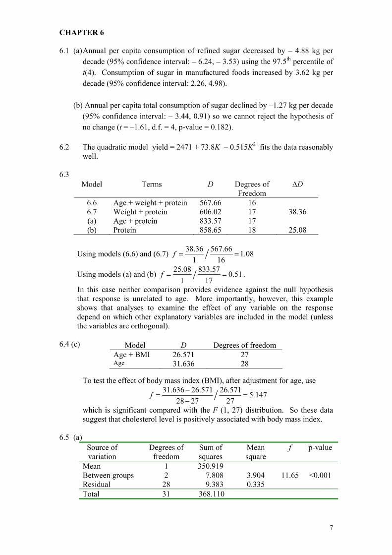
CHAPTER 6

6.1 (a) Annual per capita consumption of refined sugar decreased by – 4.88 kg per decade (95% confidence interval: – 6.24, – 3.53) using the 97.5th percentile of t(4). Consumption of sugar in manufactured foods increased by 3.62 kg per decade (95% confidence interval: 2.26, 4.98).

(b) Annual per capita total consumption of sugar declined by –1.27 kg per decade

(95% confidence interval: – 3.44, 0.91) so we cannot reject the hypothesis of no change (t = –1.61, d.f. = 4, p-value = 0.182).

6.2 The quadratic model yield = 2471 + 73.8K – 0.515K2 fits the data reasonably

well. 6.3

Model Terms D Degrees of Freedom

∆D

6.6 6.7 (a) (b)

Age + weight + protein Weight + protein Age + protein Protein

567.66 606.02 833.57 858.65

16 17 17 18

38.36

25.08

Using models (6.6) and (6.7) 38.36 567.66 1.081 16/f = =

Using models (a) and (b) 25.08 833.57 0.511 17/f = = .

In this case neither comparison provides evidence against the null hypothesis that response is unrelated to age. More importantly, however, this example shows that analyses to examine the effect of any variable on the response depend on which other explanatory variables are included in the model (unless the variables are orthogonal).

6.4 (c) Model D Degrees of freedom

Age + BMI Age

26.571 31.636

27 28

To test the effect of body mass index (BMI), after adjustment for age, use 31.636 26.571 26.571 5.147

28 27 27/f −= =

−

which is significant compared with the F (1, 27) distribution. So these data suggest that cholesterol level is positively associated with body mass index.

6.5 (a)

Source of variation

Degrees of freedom

Sum of squares

Mean square

f p-value

Mean 1 350.919 Between groups 2 7.808 3.904 11.65 <0.001 Residual 28 9.383 0.335 Total 31 368.110

7

Compared with the F (2, 28) distribution the value of f = 11.65 is very significant so we conclude the group means are not all equal. Further analyses are needed to find which means differ.

(b) Using the pooled standard deviation s = 0.5789 (from all groups) and the

97.5th percentage point for t (28), the 95% confidence interval is given by

( ) 1 13.9455 3.4375 2.048 0.578911 8

− ± × + , i.e. (–0.043, 1.059)

6.6

Source of variation Degrees of freedom

Sum of squares

Mean square

f p-value

Mean 1 51122.50 Between workers 3 54.62 18.21 14.45 <0.001 Between days 1 6.08 6.08 4.83 <0.05 Interaction 3 2.96 0.99 0.79 Residual 32 40.20 1.26 Total 40 51226.36

There are significant differences between workers and between days but no

evidence of interaction effects. 6.7

Model Deviance Degrees of freedom ( )j k jkμ α β αβ+ + + 5.00 4

j kμ α β+ + 6.07 6

jμ α+ 8.75 7

kμ β+ 24.33 8 μ 26.00 9

(a) 6.07 5 5 0.432 4/f −

= = so there is no evidence of interaction;

(b) (i) ΔD = 18.26;

(ii) ΔD = 17.25. The data are unbalanced so the model effects are not orthogonal.

6.8

Model Deviance Degrees of freedom j j xμ α+ 9.36 15

j xμ α+ 10.30 17 xμ α+ 27.23 19

jμ 26.86 18 μ 63.81 20

8

(a) 63.81 26.86 26.86 12.382 18/f −

= = which indicates that the treatment effects

are significantly different, if the initial aptitude is ignored.

(b) 10.30 9.63 9.63 0.522 15/f −

= = so there is no evidence that initial aptitude has

different effects for different treatment groups. CHAPTER 7 7.1 If dose is defined by the lower end of each dose interval (that is, 0, 1, 10, …,

200), a good model is given by ( )ˆlogit 3.489 0.0144 doseπ = − + .

The Hosmer Lemeshow test of goodness of fit can be obtained from the

following table of observed and expected frequencies (the expected

frequencies are shown in brackets)

This gives 2HLX = 0.374, d. f. = 1, p-value = 0.54 indicating a good fit.

dose leukemia other cancer

0 13 (11.6) 378 (379.4)

1 – 49 10 (11.5) 351 (349.5)

50+ 25 (24.9) 111 (111.1)

7.2 (a) if and only if ( )1 2exp 1φ β β= − = 1 2β β= .

(b) ( ) (1 2 1 2expj jx )φ α α β β⎡ ⎤= − + −⎣ ⎦ is constant if 1 2β β= 7.3 Overall the percentage of women who survived 50 years after graduation

(84%) was higher than the percentage of men who survived (67%). (a) No evidence of differences between years of graduation.

(b) and (c) Higher proportions of science graduates of either sex survived than graduates of other faculties.

(d) The effect seems more pronounced for men (ratio of proportions = 1.40) than for women (ratio = 1.18) but this is not statistically significant.

7.4 (a) ( ) ( ) ( ) ( )0 1 max min max2 2D D l b l b l b l b C− = − − − =⎡ ⎤ ⎡⎣ ⎦ ⎣ ⎤⎦

(b) For this hypothesis ( ) ( )2 20 1~ 1 , ~D N D Nχ χ p− − so ( )2 . ~ 1C pχ −

9

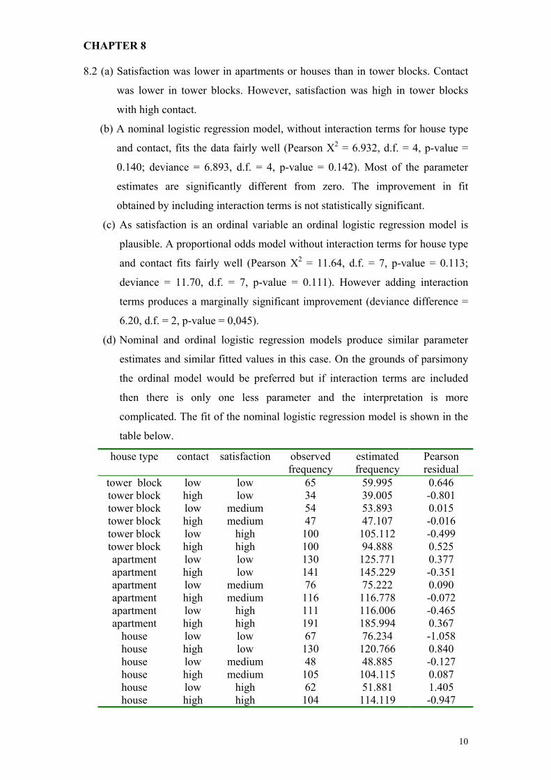
CHAPTER 8 8.2 (a) Satisfaction was lower in apartments or houses than in tower blocks. Contact

was lower in tower blocks. However, satisfaction was high in tower blocks

with high contact.

(b) A nominal logistic regression model, without interaction terms for house type

and contact, fits the data fairly well (Pearson X2 = 6.932, d.f. = 4, p-value =

0.140; deviance = 6.893, d.f. = 4, p-value = 0.142). Most of the parameter

estimates are significantly different from zero. The improvement in fit

obtained by including interaction terms is not statistically significant.

(c) As satisfaction is an ordinal variable an ordinal logistic regression model is

plausible. A proportional odds model without interaction terms for house type

and contact fits fairly well (Pearson X2 = 11.64, d.f. = 7, p-value = 0.113;

deviance = 11.70, d.f. = 7, p-value = 0.111). However adding interaction

terms produces a marginally significant improvement (deviance difference =

6.20, d.f. = 2, p-value = 0,045).

(d) Nominal and ordinal logistic regression models produce similar parameter

estimates and similar fitted values in this case. On the grounds of parsimony

the ordinal model would be preferred but if interaction terms are included

then there is only one less parameter and the interpretation is more

complicated. The fit of the nominal logistic regression model is shown in the

table below.

house type contact satisfaction observed frequency

estimated frequency

Pearson residual

tower block low low 65 59.995 0.646 tower block high low 34 39.005 -0.801 tower block low medium 54 53.893 0.015 tower block high medium 47 47.107 -0.016 tower block low high 100 105.112 -0.499 tower block high high 100 94.888 0.525 apartment low low 130 125.771 0.377 apartment high low 141 145.229 -0.351 apartment low medium 76 75.222 0.090 apartment high medium 116 116.778 -0.072 apartment low high 111 116.006 -0.465 apartment high high 191 185.994 0.367

house low low 67 76.234 -1.058 house high low 130 120.766 0.840 house low medium 48 48.885 -0.127 house high medium 105 104.115 0.087 house low high 62 51.881 1.405 house high high 104 114.119 -0.947

10

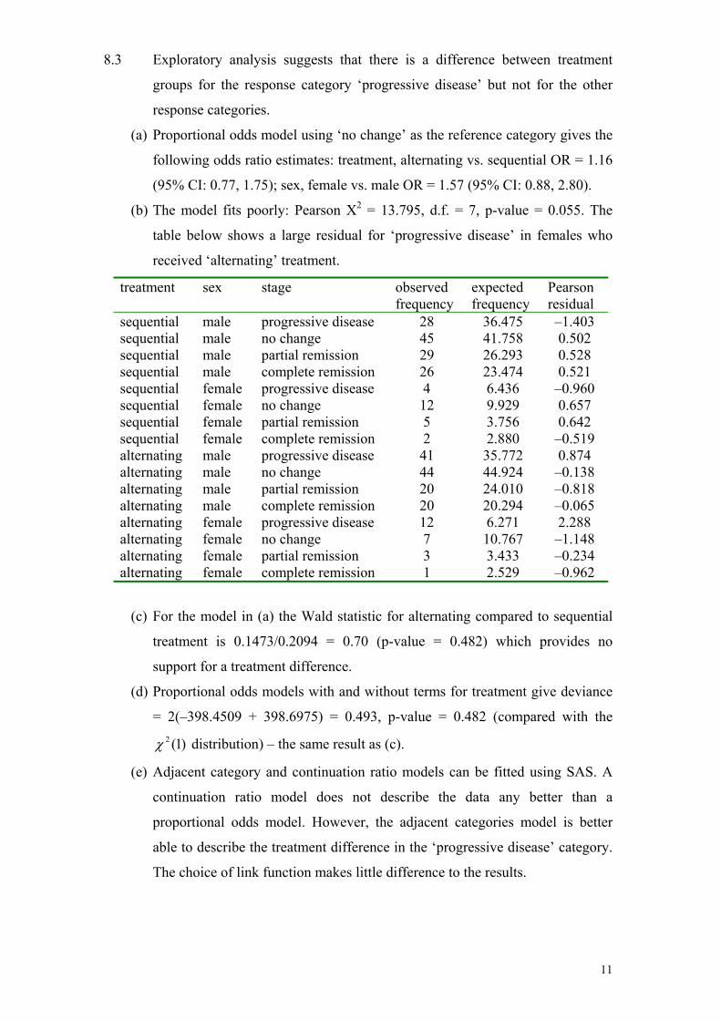
8.3 Exploratory analysis suggests that there is a difference between treatment

groups for the response category ‘progressive disease’ but not for the other

response categories.

(a) Proportional odds model using ‘no change’ as the reference category gives the

following odds ratio estimates: treatment, alternating vs. sequential OR = 1.16

(95% CI: 0.77, 1.75); sex, female vs. male OR = 1.57 (95% CI: 0.88, 2.80).

(b) The model fits poorly: Pearson X2 = 13.795, d.f. = 7, p-value = 0.055. The

table below shows a large residual for ‘progressive disease’ in females who

received ‘alternating’ treatment.

treatment sex stage observed frequency

expected frequency

Pearson residual

sequential male progressive disease 28 36.475 –1.403 sequential male no change 45 41.758 0.502 sequential male partial remission 29 26.293 0.528 sequential male complete remission 26 23.474 0.521 sequential female progressive disease 4 6.436 –0.960 sequential female no change 12 9.929 0.657 sequential female partial remission 5 3.756 0.642 sequential female complete remission 2 2.880 –0.519 alternating male progressive disease 41 35.772 0.874 alternating male no change 44 44.924 –0.138 alternating male partial remission 20 24.010 –0.818 alternating male complete remission 20 20.294 –0.065 alternating female progressive disease 12 6.271 2.288 alternating female no change 7 10.767 –1.148 alternating female partial remission 3 3.433 –0.234 alternating female complete remission 1 2.529 –0.962

(c) For the model in (a) the Wald statistic for alternating compared to sequential

treatment is 0.1473/0.2094 = 0.70 (p-value = 0.482) which provides no

support for a treatment difference.

(d) Proportional odds models with and without terms for treatment give deviance

= 2(–398.4509 + 398.6975) = 0.493, p-value = 0.482 (compared with the 2 (1)χ distribution) – the same result as (c).

(e) Adjacent category and continuation ratio models can be fitted using SAS. A

continuation ratio model does not describe the data any better than a

proportional odds model. However, the adjacent categories model is better

able to describe the treatment difference in the ‘progressive disease’ category.

The choice of link function makes little difference to the results.

11

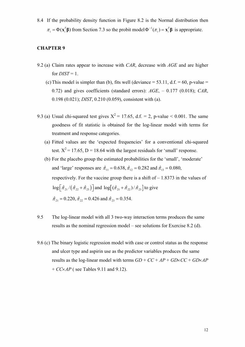
8.4 If the probability density function in Figure 8.2 is the Normal distribution then

from Section 7.3 so the probit model is appropriate. ( Ti iπ = Φ x β) 1( ) T

i iπ−Φ = x β

CHAPTER 9

9.2 (a) Claim rates appear to increase with CAR, decrease with AGE and are higher

for DIST = 1.

(c) This model is simpler than (b), fits well (deviance = 53.11, d.f. = 60, p-value =

0.72) and gives coefficients (standard errors): AGE, – 0.177 (0.018); CAR,

0.198 (0.021); DIST, 0.210 (0.059), consistent with (a).

9.3 (a) Usual chi-squared test gives X2 = 17.65, d.f. = 2, p-value < 0.001. The same

goodness of fit statistic is obtained for the log-linear model with terms for

treatment and response categories.

(a) Fitted values are the ‘expected frequencies’ for a conventional chi-squared

test. X2 = 17.65, D = 18.64 with the largest residuals for ‘small’ response.

(b) For the placebo group the estimated probabilities for the ‘small’, ‘moderate’

and ‘large’ responses are 11 12 13ˆ ˆ ˆ0.638, 0.282 and 0.080,π π π= = =

respectively. For the vaccine group there is a shift of – 1.8373 in the values of

and ( )21 22 23ˆ ˆ ˆlog /π π π⎡ ⎤+⎣ ⎦ [ ]21 22 23ˆ ˆ ˆlog ( ) /π π π+

23ˆand 0.354.

to give

21 22ˆ ˆ0.220, 0.426π π π= = =

9.5 The log-linear model with all 3 two-way interaction terms produces the same

results as the nominal regression model – see solutions for Exercise 8.2 (d).

9.6 (c) The binary logistic regression model with case or control status as the response

and ulcer type and aspirin use as the predictor variables produces the same

results as the log-linear model with terms GD + CC + AP + GD×CC + GD×AP

+ CC×AP ( see Tables 9.11 and 9.12).

12

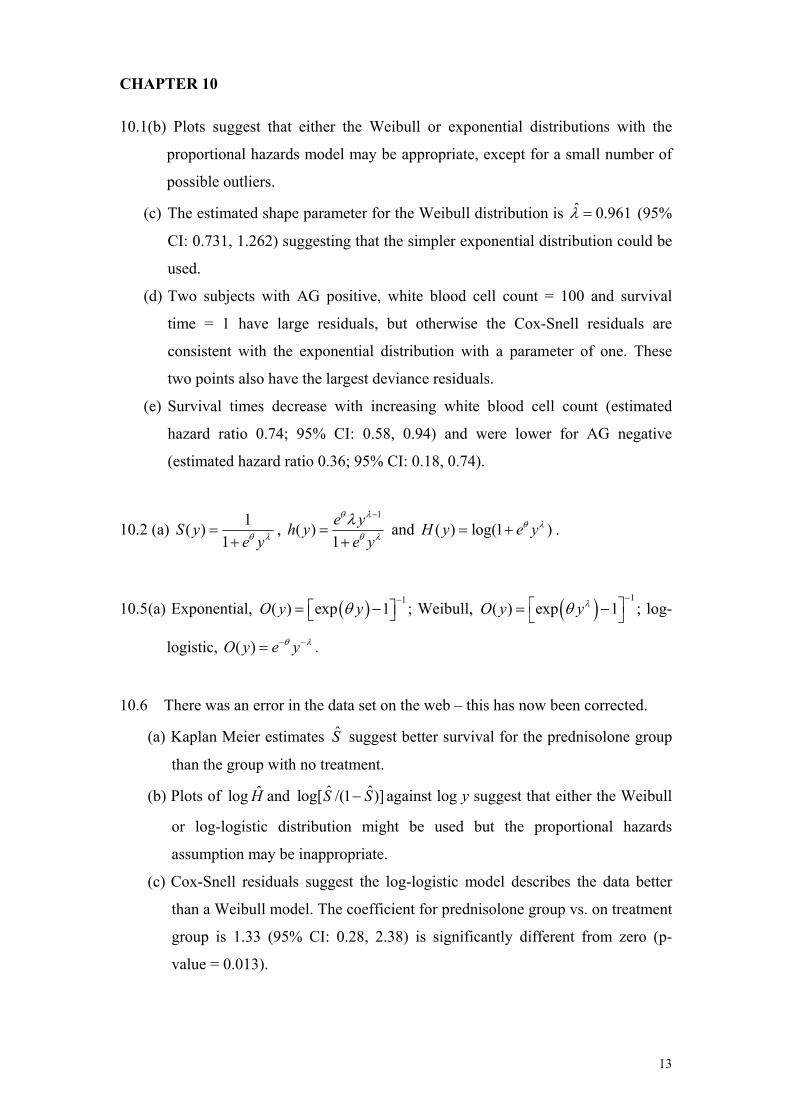
CHAPTER 10 10.1(b) Plots suggest that either the Weibull or exponential distributions with the

proportional hazards model may be appropriate, except for a small number of

possible outliers.

(c) The estimated shape parameter for the Weibull distribution is (95%

CI: 0.731, 1.262) suggesting that the simpler exponential distribution could be

used.

ˆ 0.961λ =

(d) Two subjects with AG positive, white blood cell count = 100 and survival

time = 1 have large residuals, but otherwise the Cox-Snell residuals are

consistent with the exponential distribution with a parameter of one. These

two points also have the largest deviance residuals.

(e) Survival times decrease with increasing white blood cell count (estimated

hazard ratio 0.74; 95% CI: 0.58, 0.94) and were lower for AG negative

(estimated hazard ratio 0.36; 95% CI: 0.18, 0.74).

10.2 (a) 1( )1

S ye yθ λ=

+,

1

( )1e yh y

e y

θ λ

θ λ

λ −

=+

and ( ) log(1 )H y e yθ λ= + .

10.5 (a) Exponential, ( ) 1( ) exp 1O y yθ

−⎡= −⎣ ⎤⎦ ; Weibull, ( ) 1

( ) exp 1O y yλθ−

⎡ ⎤= −⎣ ⎦ ; log-

logistic, ( )O y e yθ λ− −= .

10.6 There was an error in the data set on the web – this has now been corrected.

(a) Kaplan Meier estimates S suggest better survival for the prednisolone group

than the group with no treatment.

(b) Plots of ˆlog H and against log y suggest that either the Weibull

or log-logistic distribution might be used but the proportional hazards

assumption may be inappropriate.

ˆ ˆlog[ /(1 )]S S−

(c) Cox-Snell residuals suggest the log-logistic model describes the data better

than a Weibull model. The coefficient for prednisolone group vs. on treatment

group is 1.33 (95% CI: 0.28, 2.38) is significantly different from zero (p-

value = 0.013).

13

CHAPTER 11

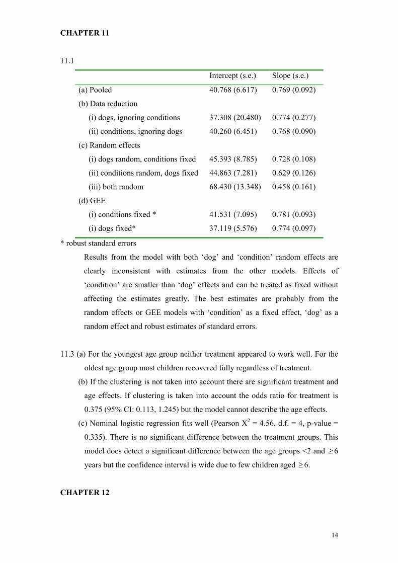
11.1

Intercept (s.e.) Slope (s.e.)

(a) Pooled 40.768 (6.617) 0.769 (0.092)

(b) Data reduction

(i) dogs, ignoring conditions 37.308 (20.480) 0.774 (0.277)

(ii) conditions, ignoring dogs 40.260 (6.451) 0.768 (0.090)

(c) Random effects

(i) dogs random, conditions fixed 45.393 (8.785) 0.728 (0.108)

(ii) conditions random, dogs fixed 44.863 (7.281) 0.629 (0.126)

(iii) both random 68.430 (13.348) 0.458 (0.161)

(d) GEE

(i) conditions fixed * 41.531 (7.095) 0.781 (0.093)

(i) dogs fixed* 37.119 (5.576) 0.774 (0.097)

* robust standard errors

Results from the model with both ‘dog’ and ‘condition’ random effects are

clearly inconsistent with estimates from the other models. Effects of

‘condition’ are smaller than ‘dog’ effects and can be treated as fixed without

affecting the estimates greatly. The best estimates are probably from the

random effects or GEE models with ‘condition’ as a fixed effect, ‘dog’ as a

random effect and robust estimates of standard errors.

11.3 (a) For the youngest age group neither treatment appeared to work well. For the

oldest age group most children recovered fully regardless of treatment.

(b) If the clustering is not taken into account there are significant treatment and

age effects. If clustering is taken into account the odds ratio for treatment is

0.375 (95% CI: 0.113, 1.245) but the model cannot describe the age effects.

(c) Nominal logistic regression fits well (Pearson X2 = 4.56, d.f. = 4, p-value =

0.335). There is no significant difference between the treatment groups. This

model does detect a significant difference between the age groups <2 and ≥6

years but the confidence interval is wide due to few children aged 6. ≥

CHAPTER 12

14

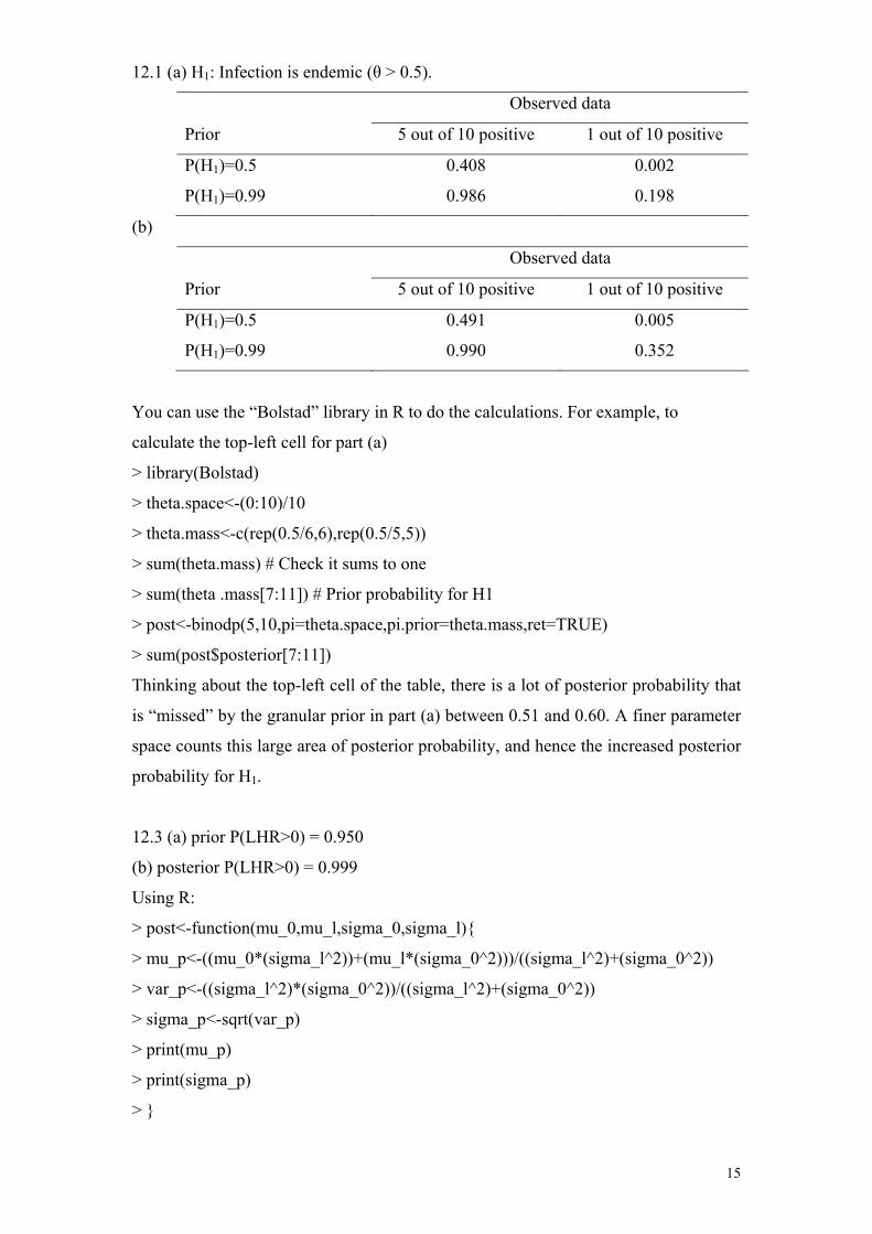
12.1 (a) H1: Infection is endemic (θ > 0.5).

Observed data

Prior 5 out of 10 positive 1 out of 10 positive

P(H1)=0.5 0.408 0.002

P(H1)=0.99 0.986 0.198

(b)

Observed data

Prior 5 out of 10 positive 1 out of 10 positive

P(H1)=0.5 0.491 0.005

P(H1)=0.99 0.990 0.352

You can use the “Bolstad” library in R to do the calculations. For example, to

calculate the top-left cell for part (a)

> library(Bolstad)

> theta.space<-(0:10)/10

> theta.mass<-c(rep(0.5/6,6),rep(0.5/5,5))

> sum(theta.mass) # Check it sums to one

> sum(theta .mass[7:11]) # Prior probability for H1

> post<-binodp(5,10,pi=theta.space,pi.prior=theta.mass,ret=TRUE)

> sum(post$posterior[7:11])

Thinking about the top-left cell of the table, there is a lot of posterior probability that

is “missed” by the granular prior in part (a) between 0.51 and 0.60. A finer parameter

space counts this large area of posterior probability, and hence the increased posterior

probability for H1.

12.3 (a) prior P(LHR>0) = 0.950

(b) posterior P(LHR>0) = 0.999

Using R:

> post<-function(mu_0,mu_l,sigma_0,sigma_l){

> mu_p<-((mu_0*(sigma_l^2))+(mu_l*(sigma_0^2)))/((sigma_l^2)+(sigma_0^2))

> var_p<-((sigma_l^2)*(sigma_0^2))/((sigma_l^2)+(sigma_0^2))

> sigma_p<-sqrt(var_p)

> print(mu_p)

> print(sigma_p)

> }

15

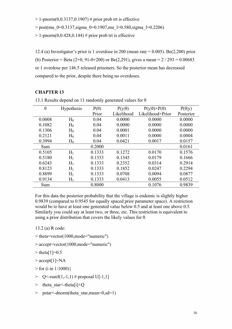
> 1-pnorm(0,0.3137,0.1907) # prior prob trt is effective

> post(mu_0=0.3137,sigma_0=0.1907,mu_l=0.580,sigma_l=0.2206)

> 1-pnorm(0,0.428,0.144) # prior prob trt is effective

12.4 (a) Investigator’s prior is 1 overdose in 200 (mean rate = 0.005). Be(2,200) prior.

(b) Posterior = Beta (2+0, 91-0+200) or Be(2,291), gives a mean = 2 / 293 = 0.00683

or 1 overdose per 146.5 released prisoners. So the posterior mean has decreased

compared to the prior, despite there being no overdoses.

CHAPTER 13

13.1 Results depend on 11 randomly generated values for θ

θ Hypothesis P(θ) Prior

P(y|θ) Likelihood

P(y|θ)×P(θ) Likelihood×Prior

P(θ|y) Posterior

0.0008 H0 0.04 0.0000 0.0000 0.0000 0.1082 H0 0.04 0.0000 0.0000 0.0000 0.1306 H0 0.04 0.0001 0.0000 0.0000 0.2121 H0 0.04 0.0011 0.0000 0.0004 0.3994 H0 0.04 0.0421 0.0017 0.0157 Sum 0.2000 0.0161

0.5105 H1 0.1333 0.1272 0.0170 0.1576 0.5180 H1 0.1333 0.1345 0.0179 0.1666 0.6243 H1 0.1333 0.2352 0.0314 0.2914 0.8123 H1 0.1333 0.1852 0.0247 0.2294 0.8899 H1 0.1333 0.0708 0.0094 0.0877 0.9134 H1 0.1333 0.0413 0.0055 0.0512 Sum 0.8000 0.1076 0.9839

For this data the posterior probability that the village is endemic is slightly higher 0.9839 (compared to 0.9545 for equally spaced prior parameter space). A restriction would be to have at least one generated value below 0.5 and at least one above 0.5. Similarly you could say at least two, or three, etc. This restriction is equivalent to using a prior distribution that covers the likely values for θ. 13.2 (a) R code:

> theta=vector(1000,mode="numeric")

> accept=vector(1000,mode="numeric")

> theta[1]=0.5

> accept[1]=NA

> for (i in 1:1000){

> Q<-runif(1,-1,1) # proposal U[-1,1]

> theta_star<-theta[i]+Q

> pstar<-dnorm(theta_star,mean=0,sd=1)

16

> p<-dnorm(theta[i],mean=0,sd=1)

> alpha<-min(pstar/p,1)

> U<-runif(1,0,1) # acceptance r.v.

> if (U>=alpha){theta[i+1]=theta[i]

> accept[i]=0}

> if (U<alpha){theta[i+1]=theta_star

> accept[i]=1}

> }

> sum(accept[2:1000])/999 # acceptance probability

> hist(theta)

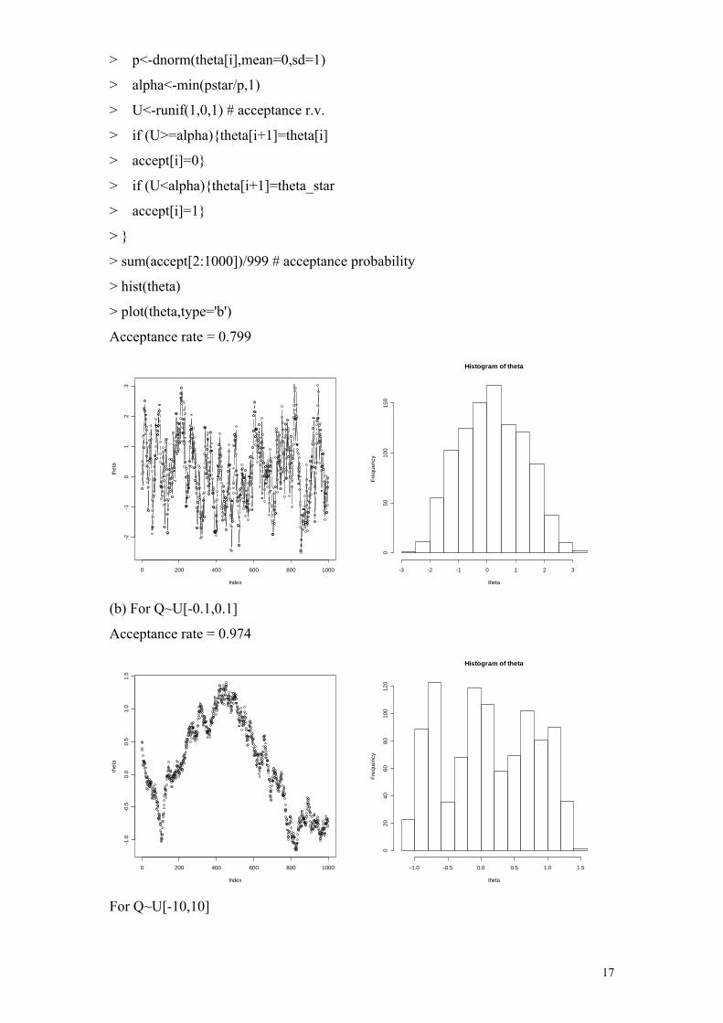
> plot(theta,type='b')

Acceptance rate = 0.799

0 200 400 600 800 1000

-2-1

01

23

Index

thet

a

Histogram of theta

theta

Freq

uenc

y

-3 -2 -1 0 1 2 3

050

100

150

(b) For Q~U[-0.1,0.1]

Acceptance rate = 0.974

0 200 400 600 800 1000

-1.0

-0.5

0.0

0.5

1.0

1.5

Index

thet

a

Histogram of theta

theta

Freq

uenc

y

-1.0 -0.5 0.0 0.5 1.0 1.5

020

4060

8010

012

0

For Q~U[-10,10]

17

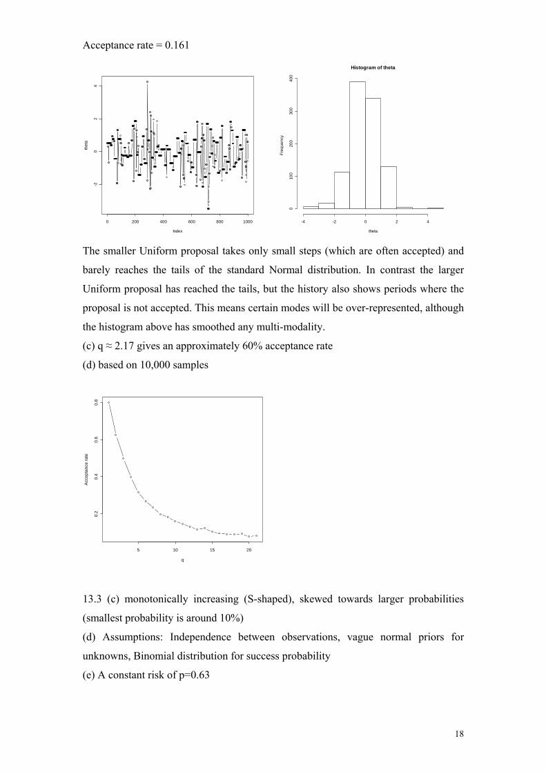
Acceptance rate = 0.161

0 200 400 600 800 1000

-20

24

Index

thet

a

Histogram of theta

theta

Freq

uenc

y

-4 -2 0 2 4

010

020

030

040

0

The smaller Uniform proposal takes only small steps (which are often accepted) and

barely reaches the tails of the standard Normal distribution. In contrast the larger

Uniform proposal has reached the tails, but the history also shows periods where the

proposal is not accepted. This means certain modes will be over-represented, although

the histogram above has smoothed any multi-modality.

(c) q ≈ 2.17 gives an approximately 60% acceptance rate

(d) based on 10,000 samples

5 10 15 20

0.2

0.4

0.6

0.8

q

Acc

epta

nce

rate

13.3 (c) monotonically increasing (S-shaped), skewed towards larger probabilities

(smallest probability is around 10%)

(d) Assumptions: Independence between observations, vague normal priors for

unknowns, Binomial distribution for success probability

(e) A constant risk of p=0.63

18

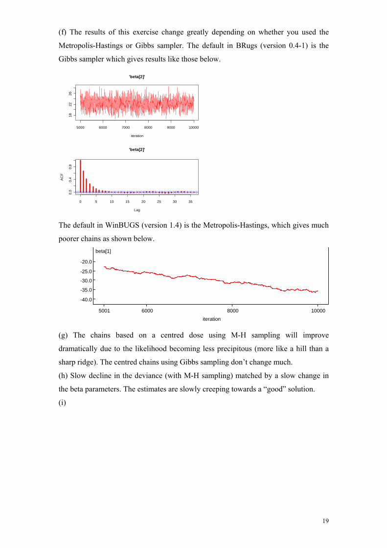
(f) The results of this exercise change greatly depending on whether you used the

Metropolis-Hastings or Gibbs sampler. The default in BRugs (version 0.4-1) is the

Gibbs sampler which gives results like those below.

5000 6000 7000 8000 9000 10000

1822

26

'beta[2]'

iteration

0 5 10 15 20 25 30 35

0.0

0.4

0.8

Lag

AC

F

'beta[2]'

The default in WinBUGS (version 1.4) is the Metropolis-Hastings, which gives much

poorer chains as shown below. beta[1]

iteration5001 6000 8000 10000

-40.0

-35.0

-30.0

-25.0

-20.0

(g) The chains based on a centred dose using M-H sampling will improve

change in

dramatically due to the likelihood becoming less precipitous (more like a hill than a

sharp ridge). The centred chains using Gibbs sampling don’t change much.

(h) Slow decline in the deviance (with M-H sampling) matched by a slow

the beta parameters. The estimates are slowly creeping towards a “good” solution.

(i)

19

0

10

20

30

40

50

60

70

1.65 1.7 1.75 1.8 1.85 1.9

Dose

Num

ber d

ead

fittedobserved

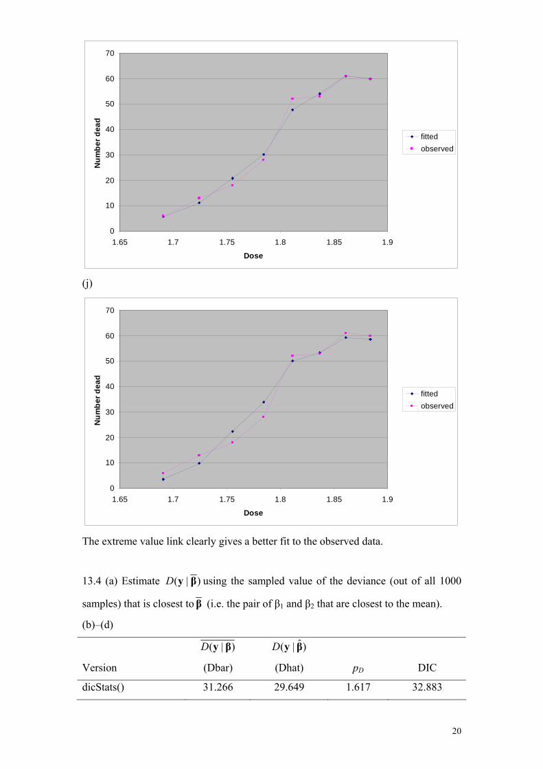
(j)

0

10

20

30

40

50

60

70

1.65 1.7 1.75 1.8 1.85 1.9

Dose

Num

ber d

ead

fittedobserved

The extreme value link clearly gives a better fit to the observed data.

13.4 (a) Estimate )|( βyD using the sampled value of the deviance (out of all 1000

samples) that is closest to β (i.e. the pair of β1 and β2 that are closest to the mean).

(b)–(d)

Version

)|( βyD

(Dbar)

)ˆ|( βyD

(Dhat) pD DIC

dicStats() 31.266 29.649 1.617 32.883

20

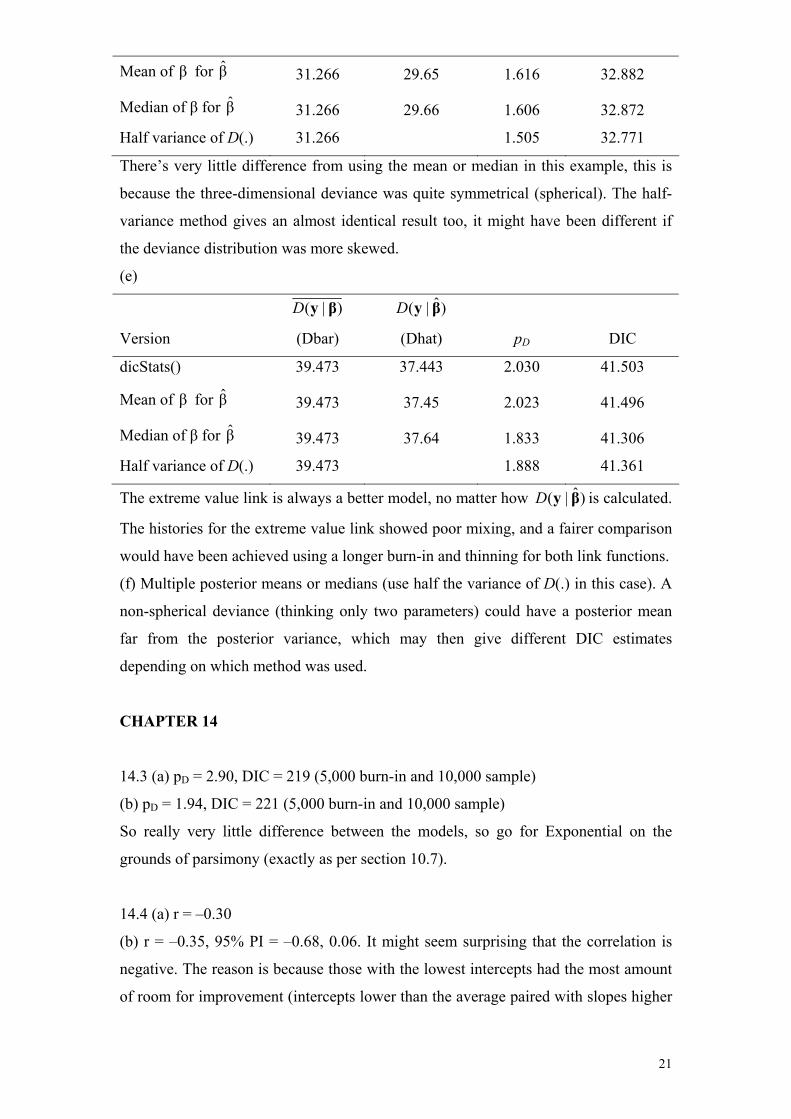
Mean of β for β ˆ 31.266 29.65 1.616 32.882

Median of β for β ˆ 31.266 29.66 1.606 32.872

Half variance of D(.) 31.266 1.505 32.771

There’s very little difference from using the mean or median in this example, this is

because the three-dimensional deviance was quite symmetrical (spherical). The half-

variance method gives an almost identical result too, it might have been different if

the deviance distribution was more skewed.

(e)

Version

)|( βyD

(Dbar)

)ˆ|( βyD

(Dhat) pD DIC

dicStats() 39.473 37.443 2.030 41.503

Mean of β for β ˆ 39.473 37.45 2.023 41.496

Median of β for β ˆ 39.473 37.64 1.833 41.306

Half variance of D(.) 39.473 1.888 41.361

The extreme value link is always a better model, no matter how is calculated.

The histories for the extreme value link showed poor mixing, and a fairer comparison

would have been achieved using a longer burn-in and thinning for both link functions.

)ˆ|( βyD

(f) Multiple posterior means or medians (use half the variance of D(.) in this case). A

non-spherical deviance (thinking only two parameters) could have a posterior mean

far from the posterior variance, which may then give different DIC estimates

depending on which method was used.

CHAPTER 14

14.3 (a) pD = 2.90, DIC = 219 (5,000 burn-in and 10,000 sample)

(b) pD = 1.94, DIC = 221 (5,000 burn-in and 10,000 sample)

So really very little difference between the models, so go for Exponential on the

grounds of parsimony (exactly as per section 10.7).

14.4 (a) r = –0.30

(b) r = –0.35, 95% PI = –0.68, 0.06. It might seem surprising that the correlation is

negative. The reason is because those with the lowest intercepts had the most amount

of room for improvement (intercepts lower than the average paired with slopes higher

21

than the average). Conversely those who were already scoring close to 100 had little

room for improvement (intercepts higher than the average paired with slopes lower

than the average).

14.5

(b)

model{

# likelihood

for(subject in 1:N) { # loop in subject

ability[subject,1:T] ~ dmnorm(mu[subject,1:T],omega.obs[1:T,1:T]);

for(time in 1:T) { # loop in time

mu[subject,time] <- alpha.c[group[subject]] +

(beta[group[subject]]*time);

} # end of time loop

} # end of subject loop

# inverse variance-covariance matrix

omega.obs[1,1] <- tau.obs; omega.obs[T,T] <- tau.obs;

for (j in 2:T-1){ omega.obs[j, j] <- tau.obs*(1+pow(rho,2));} # diagonal

for (j in 1:T-1){ omega.obs[j, j+1] <- -tau.obs*rho;

omega.obs[j+1, j] <- omega.obs[j, j+1];} # symmetry

for (i in 1:T-1) {

for (j in 2+i:T) {

omega.obs[i, j] <- 0; omega.obs[j, i] <- 0;

}

}

# priors

tau.obs ~ dgamma(0.001,0.001);

rho~dunif(-0.99,0.99); # correlation parameter

beta[1] ~ dnorm(0,1.0E-4); # Linear effect of time (group=A)

beta[2] ~ dnorm(0,1.0E-4);

beta[3] ~ dnorm(0,1.0E-4);

alpha.c[1]~dnorm(0,1.0E-4); # Centred intercept (group=A)

alpha.c[2]~dnorm(0,1.0E-4);

alpha.c[3]~dnorm(0,1.0E-4);

# scalars

22

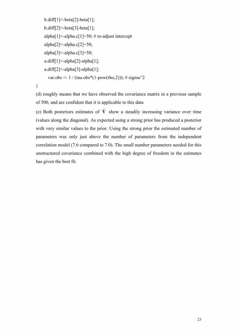
b.diff[1]<-beta[2]-beta[1];

b.diff[2]<-beta[3]-beta[1];

alpha[1]<-alpha.c[1]+50; # re-adjust intercept

alpha[2]<-alpha.c[2]+50;

alpha[3]<-alpha.c[3]+50;

a.diff[1]<-alpha[2]-alpha[1];

a.diff[2]<-alpha[3]-alpha[1];

var.obs <- 1 / (tau.obs*(1-pow(rho,2))); # sigma^2

}

(d) roughly means that we have observed the covariance matrix in a previous sample

of 500, and are confident that it is applicable to this data

(e) Both posteriors estimates of show a steadily increasing variance over time

(values along the diagonal). As expected using a strong prior has produced a posterior

with very similar values to the prior. Using the strong prior the estimated number of

parameters was only just above the number of parameters from the independent

correlation model (7.6 compared to 7.0). The small number parameters needed for this

unstructured covariance combined with the high degree of freedom in the estimates

has given the best fit.

V

23