UVA CS 4774: Machine Learning Lecture 5: Linear Regression ...
Simple LinearRegression II
Parameter Estimation
Residual Analysis
Confidence/PredictionIntervals
Hypothesis Testing
2.1
Lecture 2Simple Linear Regression IIReading: Chapter 11
STAT 8020 Statistical Methods IIAugust 25, 2020
Whitney HuangClemson University

Simple LinearRegression II
Parameter Estimation
Residual Analysis
Confidence/PredictionIntervals
Hypothesis Testing
2.2
Agenda
1 Parameter Estimation
2 Residual Analysis
3 Confidence/Prediction Intervals
4 Hypothesis Testing
Simple LinearRegression II
Parameter Estimation
Residual Analysis
Confidence/PredictionIntervals
Hypothesis Testing
2.3
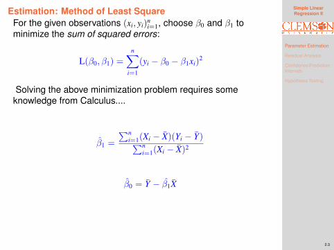
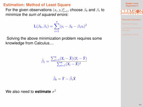
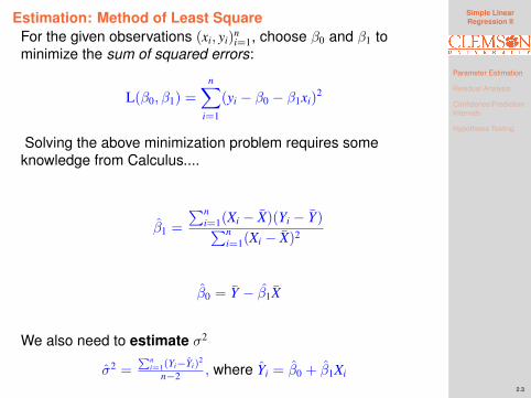
Estimation: Method of Least SquareFor the given observations (xi, yi)
ni=1, choose β0 and β1 to
minimize the sum of squared errors:
L(β0, β1) =
n∑i=1
(yi − β0 − β1xi)2
Solving the above minimization problem requires someknowledge from Calculus....
β1 =
∑ni=1(Xi − X)(Yi − Y)∑n
i=1(Xi − X)2
β0 = Y − β1X
We also need to estimate σ2
σ2 =∑n
i=1(Yi−Yi)2
n−2 , where Yi = β0 + β1Xi
Simple LinearRegression II
Parameter Estimation
Residual Analysis
Confidence/PredictionIntervals
Hypothesis Testing
2.3
Estimation: Method of Least SquareFor the given observations (xi, yi)
ni=1, choose β0 and β1 to
minimize the sum of squared errors:
L(β0, β1) =
n∑i=1
(yi − β0 − β1xi)2
Solving the above minimization problem requires someknowledge from Calculus....
β1 =
∑ni=1(Xi − X)(Yi − Y)∑n
i=1(Xi − X)2
β0 = Y − β1X
We also need to estimate σ2
σ2 =∑n
i=1(Yi−Yi)2
n−2 , where Yi = β0 + β1Xi
Simple LinearRegression II
Parameter Estimation
Residual Analysis
Confidence/PredictionIntervals
Hypothesis Testing
2.4
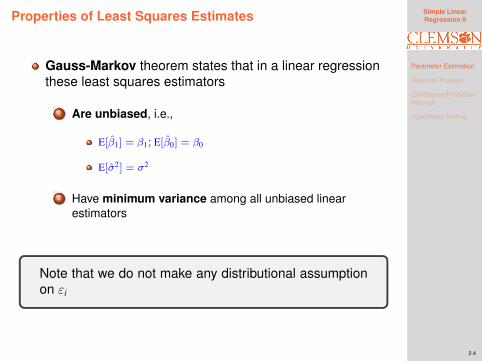
Properties of Least Squares Estimates
Gauss-Markov theorem states that in a linear regressionthese least squares estimators
1 Are unbiased, i.e.,
E[β1] = β1; E[β0] = β0
E[σ2] = σ2
2 Have minimum variance among all unbiased linearestimators
Note that we do not make any distributional assumptionon εi
Simple LinearRegression II
Parameter Estimation
Residual Analysis
Confidence/PredictionIntervals
Hypothesis Testing
2.5
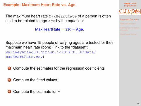
Example: Maximum Heart Rate vs. Age
The maximum heart rate MaxHeartRate of a person is oftensaid to be related to age Age by the equation:
MaxHeartRate = 220− Age.
Suppose we have 15 people of varying ages are tested for theirmaximum heart rate (bpm) (link to the “dataset":whitneyhuang83.github.io/STAT8010/Data/maxHeartRate.csv)
1 Compute the estimates for the regression coefficients
2 Compute the fitted values
3 Compute the estimate for σ
Simple LinearRegression II
Parameter Estimation
Residual Analysis
Confidence/PredictionIntervals
Hypothesis Testing
2.6
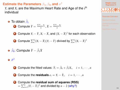
Estimate the Parameters β1, β0, and σ2
Yi and Xi are the Maximum Heart Rate and Age of the ith
individual
To obtain β1
1 Compute Y =∑n
i=1 Yin , X =
∑ni=1 Xi
n
2 Compute Yi − Y, Xi − X, and (Xi − X)2 for each observation
3 Compute∑n
i (Xi − X)(Yi − Y) divived by∑n
i (Xi − X)2
β0: Compute Y − β1X
σ2
1 Compute the fitted values: Yi = β0 + β1Xi, i = 1, · · · , n
2 Compute the residuals ei = Yi − Yi, i = 1, · · · , n
3 Compute the residual sum of squares (RSS)=∑n
i=1(Yi − Yi)2 and divided by n− 2 (why?)
Simple LinearRegression II
Parameter Estimation
Residual Analysis
Confidence/PredictionIntervals
Hypothesis Testing
2.7
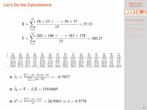
Let’s Do the Calculations
X =
15∑i=1
18 + 23 + · · ·+ 39 + 3715
= 37.33
Y =
15∑i=1
202 + 186 + · · ·+ 183 + 17815
= 180.27
X 18 23 25 35 65 54 34 56 72 19 23 42 18 39 37Y 202 186 187 180 156 169 174 172 153 199 193 174 198 183 178
-19.33 -14.33 -12.33 -2.33 27.67 16.67 -3.33 18.67 34.67 -18.33 -14.33 4.67 -19.33 1.67 -0.3321.73 5.73 6.73 -0.27 -24.27 -11.27 -6.27 -8.27 -27.27 18.73 12.73 -6.27 17.73 2.73 -2.27
-420.18 -82.18 -83.04 0.62 -671.38 -187.78 20.89 -154.31 -945.24 -343.44 -182.51 -29.24 -342.84 4.56 0.76373.78 205.44 152.11 5.44 765.44 277.78 11.11 348.44 1201.78 336.11 205.44 21.78 373.78 2.78 0.11195.69 191.70 190.11 182.13 158.20 166.97 182.93 165.38 152.61 194.89 191.70 176.54 195.69 178.94 180.53
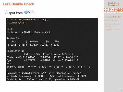
β1 =∑n
i=1(Xi−X)(Yi−Y)∑ni=1(Xi−X)2 = −0.7977
β0 = Y − β1X = 210.0485
σ2 =∑15
i=1(Yi−Yi)2
13 = 20.9563⇒ σ = 4.5778
Simple LinearRegression II
Parameter Estimation
Residual Analysis
Confidence/PredictionIntervals
Hypothesis Testing
2.8
Let’s Double Check
Output from
Simple LinearRegression II
Parameter Estimation
Residual Analysis
Confidence/PredictionIntervals
Hypothesis Testing
2.9
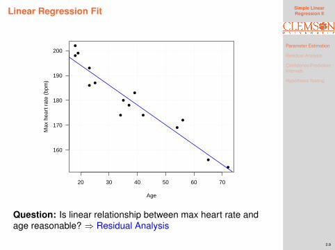
Linear Regression Fit
●
●●
●
●
●
●
●
●
●
●
●
●
●
●
20 30 40 50 60 70
160
170
180
190
200
Age
Max
hea
rt r
ate
(bpm
)
Question: Is linear relationship between max heart rate andage reasonable? ⇒ Residual Analysis
Simple LinearRegression II
Parameter Estimation
Residual Analysis
Confidence/PredictionIntervals
Hypothesis Testing
2.10
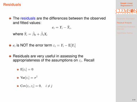
Residuals
The residuals are the differences between the observedand fitted values:
ei = Yi − Yi,
where Yi = β0 + β1Xi
ei is NOT the error term εi = Yi − E[Yi]
Residuals are very useful in assessing theappropriateness of the assumptions on εi. Recall
E[εi] = 0
Var[εi] = σ2
Cov[εi, εj] = 0, i 6= j
Simple LinearRegression II
Parameter Estimation
Residual Analysis
Confidence/PredictionIntervals
Hypothesis Testing
2.11
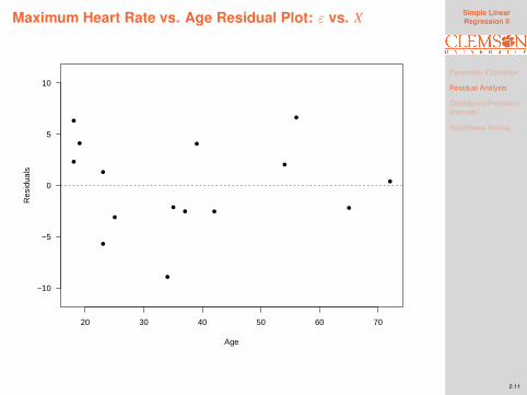
Maximum Heart Rate vs. Age Residual Plot: ε vs. X
●
●
●
● ●
●
●
●
●
●
●
●
●
●
●
20 30 40 50 60 70
−10
−5
0
5
10
Age
Res
idua
ls
Simple LinearRegression II
Parameter Estimation
Residual Analysis
Confidence/PredictionIntervals
Hypothesis Testing
2.12
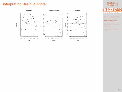
Interpreting Residual Plots
Figure: Figure courtesy of Faraway’s Linear Models with R (2005, p.59).
Simple LinearRegression II
Parameter Estimation
Residual Analysis
Confidence/PredictionIntervals
Hypothesis Testing
2.12
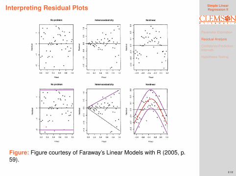
Interpreting Residual Plots
Figure: Figure courtesy of Faraway’s Linear Models with R (2005, p.59).
Simple LinearRegression II
Parameter Estimation
Residual Analysis
Confidence/PredictionIntervals
Hypothesis Testing
2.13
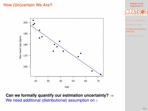
How (Un)certain We Are?
●
●●
●
●
●
●
●
●
●
●
●
●
●
●
20 30 40 50 60 70
160
170
180
190
200
Age
Max
hea
rt r
ate
(bpm
)
Can we formally quantify our estimation uncertainty? ⇒We need additional (distributional) assumption on ε
Simple LinearRegression II
Parameter Estimation
Residual Analysis
Confidence/PredictionIntervals
Hypothesis Testing
2.14
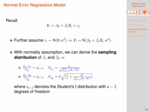
Normal Error Regression Model
RecallYi = β0 + β1Xi + εi
Further assume εi ∼ N(0, σ2)⇒ Yi ∼ N(β0 + β1Xi, σ2)
With normality assumption, we can derive the samplingdistribution of β1 and β0 ⇒
β1−β1σβ1∼ tn−2, σβ1
= σ√∑ni=1(Xi−X)2
β0−β0σβ0∼ tn−2, σβ0
= σ√
( 1n + X2∑n
i=1(Xi−X)2 )
where tn−2 denotes the Student’s t distribution with n− 2degrees of freedom
Simple LinearRegression II
Parameter Estimation
Residual Analysis
Confidence/PredictionIntervals
Hypothesis Testing
2.15
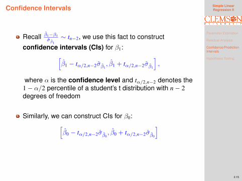
Confidence Intervals
Recall β1−β1σβ1
∼ tn−2, we use this fact to construct
confidence intervals (CIs) for β1:[β1 − tα/2,n−2σβ1
, β1 + tα/2,n−2σβ1
],
where α is the confidence level and tα/2,n−2 denotes the1− α/2 percentile of a student’s t distribution with n− 2degrees of freedom
Similarly, we can construct CIs for β0:[β0 − tα/2,n−2σβ0
, β0 + tα/2,n−2σβ0
]
Simple LinearRegression II
Parameter Estimation
Residual Analysis
Confidence/PredictionIntervals
Hypothesis Testing
2.16
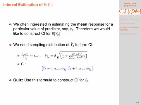
Interval Estimation of E(Yh)
We often interested in estimating the mean response for aparticular value of predictor, say, Xh. Therefore we wouldlike to construct CI for E[Yh]
We need sampling distribution of Yh to form CI:
Yh−YhσYh∼ tn−2, σYh
= σ
√(1n + (Xh−X)2∑n
i=1(Xi−X)2
)CI: [
Yh − tα/2,n−2σYh, Yh + tα/2,n−2σYh
]Quiz: Use this formula to construct CI for β0
Simple LinearRegression II
Parameter Estimation
Residual Analysis
Confidence/PredictionIntervals
Hypothesis Testing
2.17
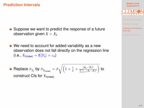
Prediction Intervals
Suppose we want to predict the response of a futureobservation given X = Xh
We need to account for added variability as a newobservation does not fall directly on the regression line(i.e., Yh(new) = E[Yh] + εh)
Replace σYhby σYh(new)
= σ
√(1 + 1
n + (Xh−X)2∑ni=1(Xi−X)2
)to
construct CIs for Yh(new)
Simple LinearRegression II
Parameter Estimation
Residual Analysis
Confidence/PredictionIntervals
Hypothesis Testing
2.18
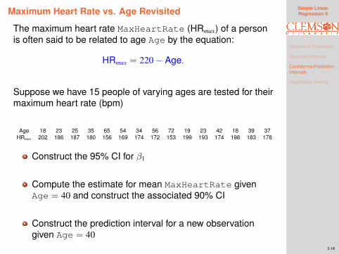
Maximum Heart Rate vs. Age Revisited
The maximum heart rate MaxHeartRate (HRmax) of a personis often said to be related to age Age by the equation:
HRmax = 220− Age.
Suppose we have 15 people of varying ages are tested for theirmaximum heart rate (bpm)
Age 18 23 25 35 65 54 34 56 72 19 23 42 18 39 37HRmax 202 186 187 180 156 169 174 172 153 199 193 174 198 183 178
Construct the 95% CI for β1
Compute the estimate for mean MaxHeartRate givenAge = 40 and construct the associated 90% CI
Construct the prediction interval for a new observationgiven Age = 40
Simple LinearRegression II
Parameter Estimation
Residual Analysis
Confidence/PredictionIntervals
Hypothesis Testing
2.19
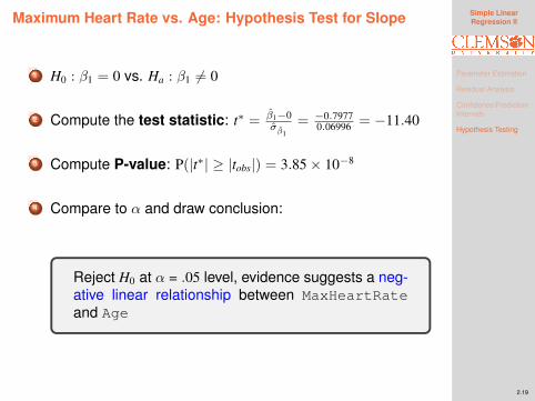
Maximum Heart Rate vs. Age: Hypothesis Test for Slope
1 H0 : β1 = 0 vs. Ha : β1 6= 0
2 Compute the test statistic: t∗ = β1−0σβ1
= −0.79770.06996 = −11.40
3 Compute P-value: P(|t∗| ≥ |tobs|) = 3.85× 10⁻⁸
4 Compare to α and draw conclusion:
Reject H0 at α = .05 level, evidence suggests a neg-ative linear relationship between MaxHeartRateand Age
Simple LinearRegression II
Parameter Estimation
Residual Analysis
Confidence/PredictionIntervals
Hypothesis Testing
2.20
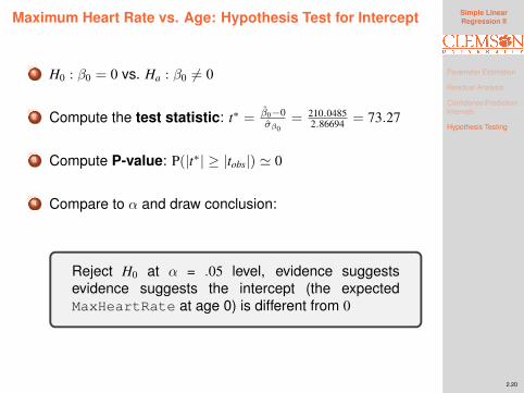
Maximum Heart Rate vs. Age: Hypothesis Test for Intercept
1 H0 : β0 = 0 vs. Ha : β0 6= 0
2 Compute the test statistic: t∗ = β0−0σβ0
= 210.04852.86694 = 73.27
3 Compute P-value: P(|t∗| ≥ |tobs|) ' 0
4 Compare to α and draw conclusion:
Reject H0 at α = .05 level, evidence suggestsevidence suggests the intercept (the expectedMaxHeartRate at age 0) is different from 0
Simple LinearRegression II
Parameter Estimation
Residual Analysis
Confidence/PredictionIntervals
Hypothesis Testing
2.21
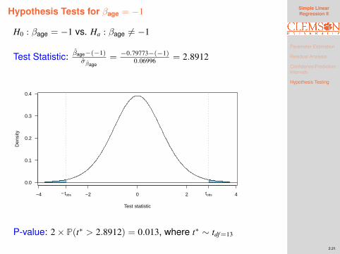
Hypothesis Tests for βage = −1
H0 : βage = −1 vs. Ha : βage 6= −1
Test Statistic: βage−(−1)σβage
= −0.79773−(−1)0.06996 = 2.8912
−4 −2 0 2 4
0.0
0.1
0.2
0.3
0.4
Test statistic
Den
sity
tobs− tobs
P-value: 2× P(t∗ > 2.8912) = 0.013, where t∗ ∼ tdf =13
Simple LinearRegression II
Parameter Estimation
Residual Analysis
Confidence/PredictionIntervals
Hypothesis Testing
2.22
Summary
In this lecture, we reviewedSimple Linear Regression: Yi = β0 + β1Xi + εi
Method of Least Square for parameter estimation
Residual analysis to check model assumptions
statistical inference for β0 and β1
Confidence/Prediction Intervals and Hypothesis TestingNext time we will talk about
1 Analysis of Variance (ANOVA) Approach to Regression
2 Correlation (r) & Coefficient of Determination (R2)