PubH 7405: REGRESSION ANALYSIS

SLR: DIAGNOSTICS & REMEDIES

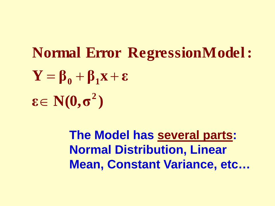
)σN(0,εεxββY

:Model RegressionError Normal

210

∈

++=

The Model has several parts: Normal Distribution, Linear Mean, Constant Variance, etc…

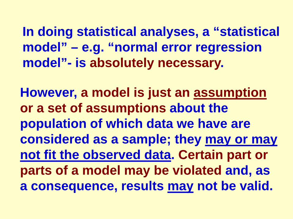
In doing statistical analyses, a “statistical model” – e.g. “normal error regression model”- is absolutely necessary.

However, a model is just an assumption or a set of assumptions about the population of which data we have are considered as a sample; they may or may not fit the observed data. Certain part or parts of a model may be violated and, as a consequence, results may not be valid.

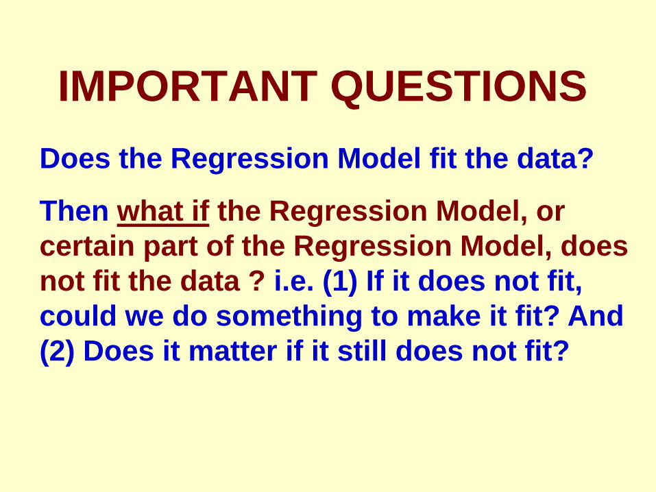
IMPORTANT QUESTIONS Does the Regression Model fit the data?

Then what if the Regression Model, or certain part of the Regression Model, does not fit the data ? i.e. (1) If it does not fit, could we do something to make it fit? And (2) Does it matter if it still does not fit?

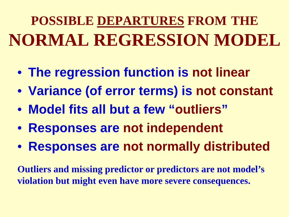
POSSIBLE DEPARTURES FROM THE NORMAL REGRESSION MODEL

• The regression function is not linear • Variance (of error terms) is not constant • Model fits all but a few “outliers” • Responses are not independent • Responses are not normally distributed Outliers and missing predictor or predictors are not model’s violation but might even have more severe consequences.

Besides the data values for the dependent and independent variables, diagnostics would be based on the “residuals” (errors of individual fitted values) and some of their transformed values.

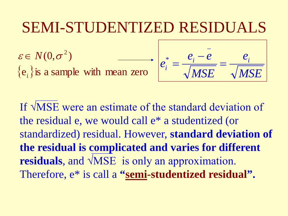
SEMI-STUDENTIZED RESIDUALS

MSEe

MSEeee ii

i =−

=

_

*

If √MSE were an estimate of the standard deviation of the residual e, we would call e* a studentized (or standardized) residual. However, standard deviation of the residual is complicated and varies for different residuals, and √MSE is only an approximation. Therefore, e* is call a “semi-studentized residual”.

{ } zeromean with sample a is e),0(

i

2σε N∈

Diagnostics could be informal using plots/graphs or could be based on formal application of statistical tests; graphical method is more popular and would be sufficient. We could perform a few statistical tests but, most of the times, they are not really necessary.

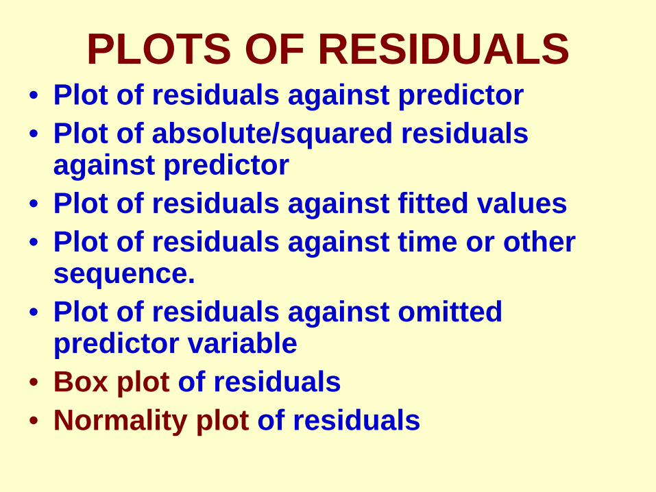
PLOTS OF RESIDUALS • Plot of residuals against predictor • Plot of absolute/squared residuals

against predictor • Plot of residuals against fitted values • Plot of residuals against time or other

sequence. • Plot of residuals against omitted

predictor variable • Box plot of residuals • Normality plot of residuals

In any of those graphs, you could plot semi-studentized residuals instead of residuals. A semi-studentized residual is a residual on “standard deviation scale”; graphs provide same type of information.

Issue: NONLINEARITY • Whether a linear regression function is appropriate for a

given data set can be studied from a scatter diagram (e.g.. Using Excel); but it’s not always effective (less visible).

• More effective to use a residual plot against the predictor variable or, equivalently, against the fitted values; if model fits, one would have a horizontal band centered around zero which has no special clustering pattern.

• The lack of fit would result in a graph showing the residuals departing from zeros in a systematic fashion – likely a curvilinear shape.

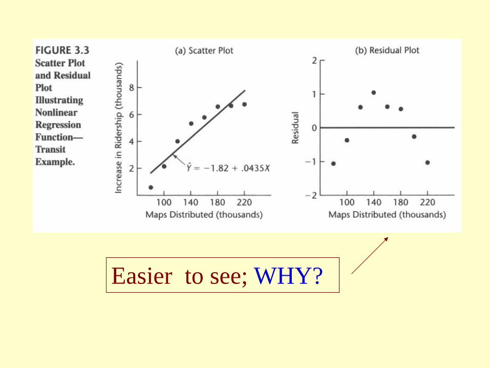
Easier to see; WHY?

REMEDIAL MEASURES • If a SLR model is found not appropriate for the

data at hand, there are two basic choices: (1) Abandon it and search for a suitable one, or (2) Use some transformation on the data to create

a fit for the transformed data • Each has advantages & disadvantages: first

approach may yield better insights but may lead to more technical difficulties; transformations are more simple but may obscure the fundamental real relationship; sometimes it’s hard to explain.

LOG TRANSFORMATIONS • Typical: Y* = Log (Y), turns a multiplicative

model into an additive model – for linearity. • Residuals should be used to check if model fits

transformed data: normality, independence, and constant variance because the distribution changes the distribution and the variance of the error terms.

• Others: (1) X* = Log (X), (2) X* = Log (X) and Y* = Log (Y); Example: Model (2) is used to study “demand” (Y) versus “price of commodity” (X) in economics.

Example:

Y* = ln(Y=PSA) is used in the model for PSA with Prostate Cancer Note: When the distribution of the error terms is close to normal with an approximately constant variance, and a transformation is needed only for linearizing a non-linear regression relation, only transformations on X should be attempted.

RECIPROCAL TRANSFORMATIONS

• Also aimed for linearity • Possibilities are: (1) X* = 1/X, (2) Y* = 1/Y, (3) X* = 1/X and Y* = 1/Y • Example: Models (1) and (2) are useful

when it seems that Y has a lower or upper “asymptote” (e.g. hourly earning)

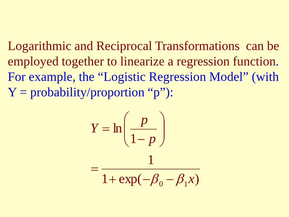
Logarithmic and Reciprocal Transformations can be employed together to linearize a regression function. For example, the “Logistic Regression Model” (with Y = probability/proportion “p”):

)exp(11

1ln

10 x

ppY

ββ −−+=

−

=

Issue: NONCONSTANCY OF VARIANCE • Scatter diagram is also helpful to see if the variance of

error terms are constant; if model fits, one would have a band with constant width centered around the regression line which has no special clustering pattern. Again, not always effective

• More effective to plot residuals (or their absolute or squared values) against the predictor variable or, equivalently, against the fitted values. If model fits, one would have a band with constant width centered around the horizontal axis. The lack of fit would result in a graph showing the residuals departing from zeros in a systematic fashion – likely a “megaphone” or “reverse megaphone” shape.

EXAMPLE: Plutonium Measurement An Example in environmental clean up;

X = Plutonium Activity (pCi/g)

Y = Alpha Count Rate (#/sec)

A full description of the example is in section 3.11, starting on page 141 (in practice its use involves an inverse prediction, predicting plutonium activity from the observed alpha count (Plutonium emits alpha particles).

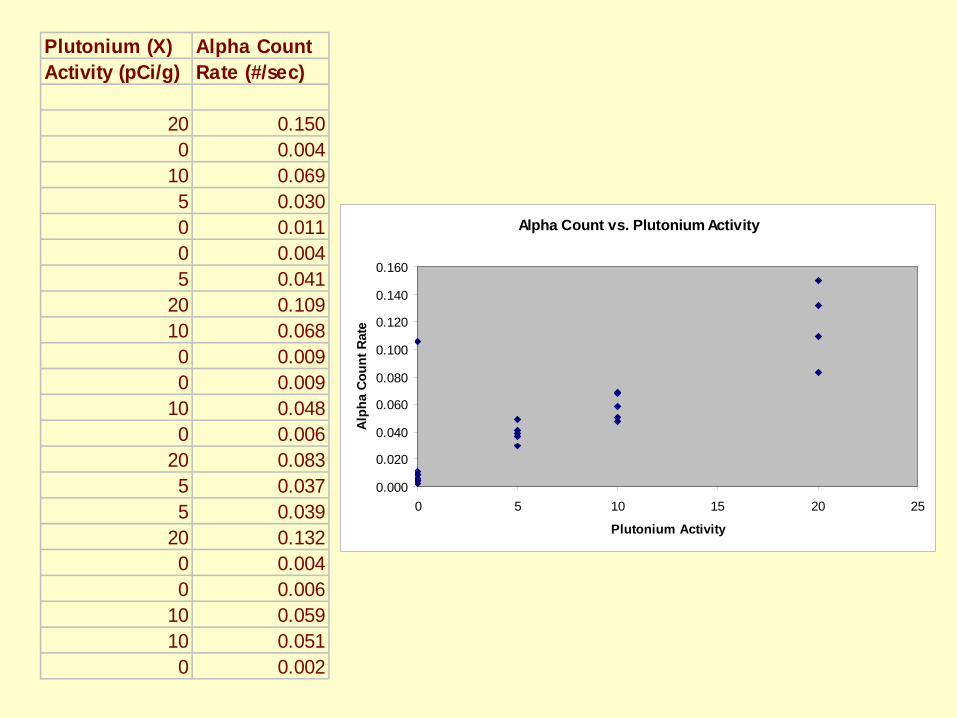
Plutonium (X) Alpha CountActivity (pCi/g) Rate (#/sec)

20 0.1500 0.004

10 0.0695 0.0300 0.0110 0.0045 0.041

20 0.10910 0.0680 0.0090 0.009

10 0.0480 0.006

20 0.0835 0.0375 0.039

20 0.1320 0.0040 0.006

10 0.05910 0.0510 0.002

Alpha Count vs. Plutonium Activity

0.000

0.020

0.040

0.060

0.080

0.100

0.120

0.140

0.160

0 5 10 15 20 25

Plutonium Activity

Alph

a Co

unt R

ate

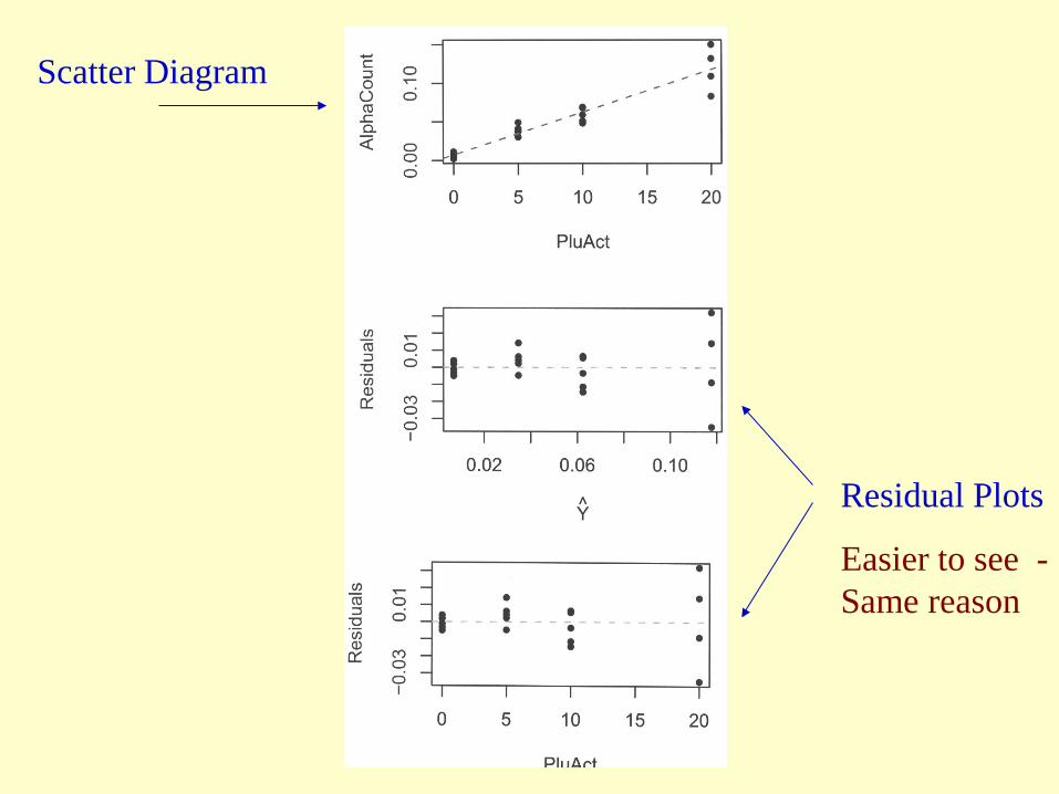
Scatter Diagram

Residual Plots

Easier to see -Same reason

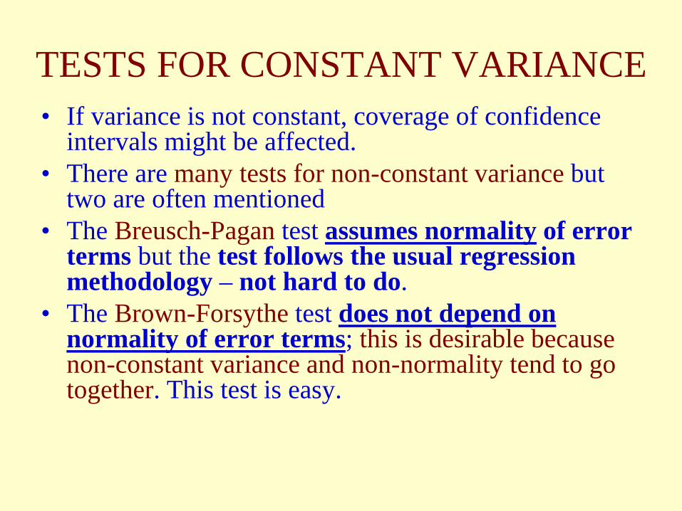
TESTS FOR CONSTANT VARIANCE • If variance is not constant, coverage of confidence

intervals might be affected. • There are many tests for non-constant variance but

two are often mentioned • The Breusch-Pagan test assumes normality of error

terms but the test follows the usual regression methodology – not hard to do.

• The Brown-Forsythe test does not depend on normality of error terms; this is desirable because non-constant variance and non-normality tend to go together. This test is easy.

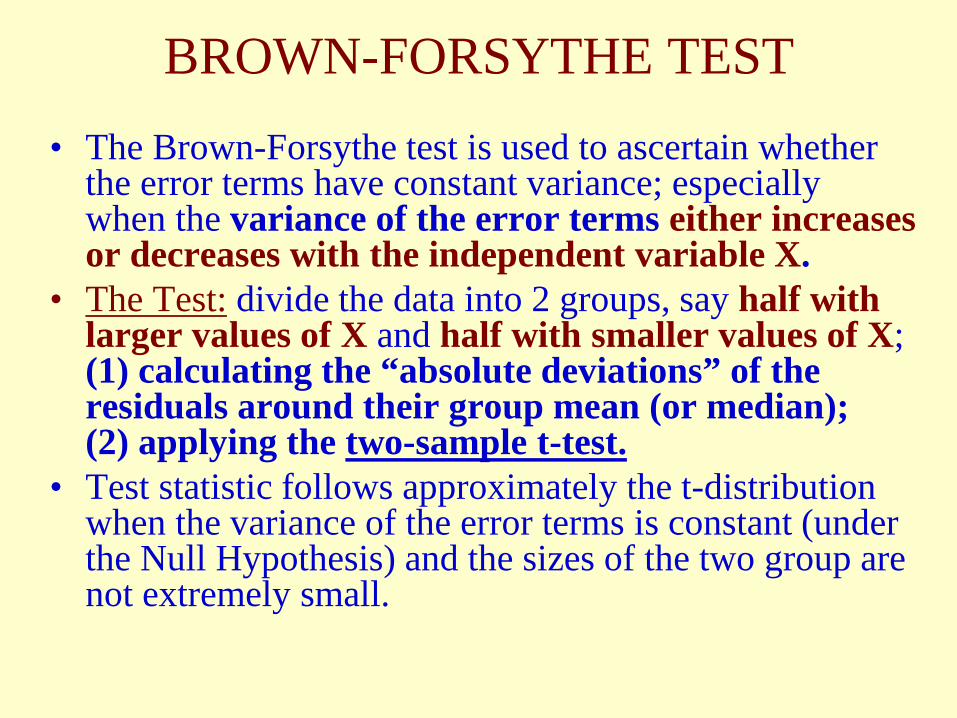
BROWN-FORSYTHE TEST • The Brown-Forsythe test is used to ascertain whether

the error terms have constant variance; especially when the variance of the error terms either increases or decreases with the independent variable X.

• The Test: divide the data into 2 groups, say half with larger values of X and half with smaller values of X; (1) calculating the “absolute deviations” of the residuals around their group mean (or median); (2) applying the two-sample t-test.

• Test statistic follows approximately the t-distribution when the variance of the error terms is constant (under the Null Hypothesis) and the sizes of the two group are not extremely small.

BROWN-FORSYTHE: RATIONALE • If the error variance is either increasing or

decreasing with X, the residuals in one group tend to be more variable than those residuals in the other.

• The Brown-Forsythe test does not assume normality of error terms; this is desirable because non-constant variance and non-normality tend to go together.

• It’s is very similar to “Levine’s test” to compare any two variances – instead of forming the ratio of two sample variances (& use “F-test”).

LotSize WorkHours80 39930 12150 22190 37670 36160 224

120 54680 352

100 35350 15740 16070 25290 38920 113

110 435100 42030 21250 26890 377

110 42130 27390 46840 24480 34270 323

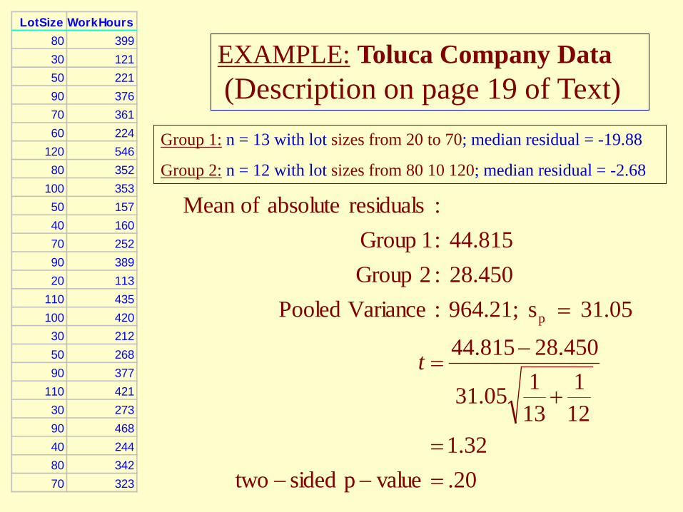
EXAMPLE: Toluca Company Data (Description on page 19 of Text)

.20valuep sidedtwo32.1

121

13105.31

450.28815.44

31.05 s 964.21; :Variance Pooled28.450 :2 Group44.815 :1 Group

:residuals absolute ofMean

p

=−−=

+

−=

=

t

Group 1: n = 13 with lot sizes from 20 to 70; median residual = -19.88

Group 2: n = 12 with lot sizes from 80 10 120; median residual = -2.68

This example shows that the half with smaller X’s has larger residuals – and vice versa; the pattern of an inverse mega phone – but it’s “not significant”, a case that makes me uneasy with statistical tests: I want to assume that the variance is constant, it only says that we do not have enough data to conclude that the variance is not constant!

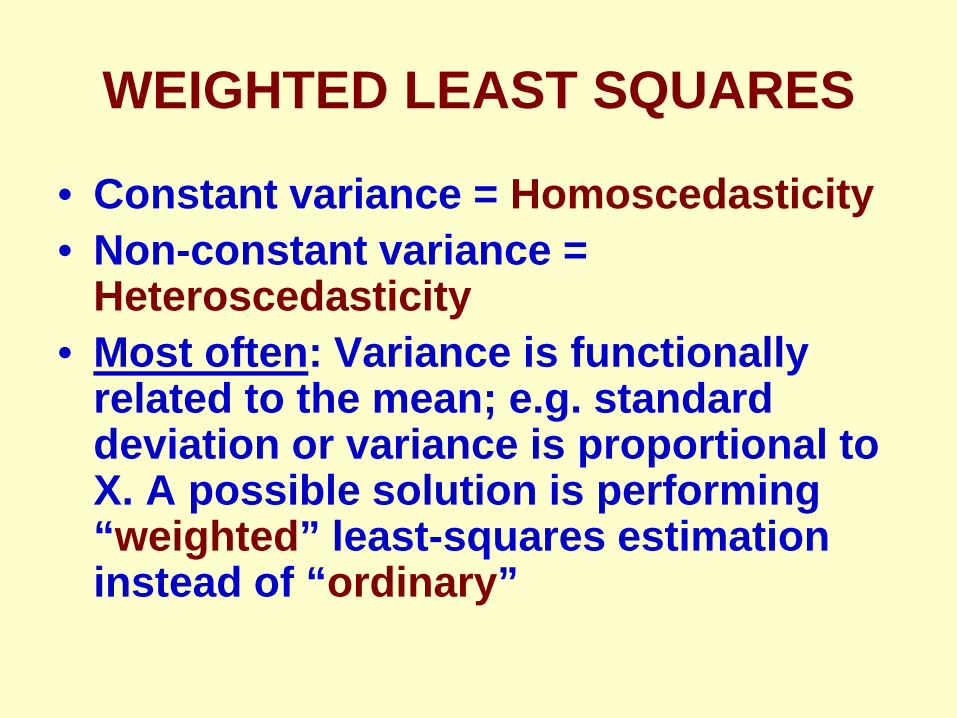
WEIGHTED LEAST SQUARES

• Constant variance = Homoscedasticity • Non-constant variance =

Heteroscedasticity • Most often: Variance is functionally

related to the mean; e.g. standard deviation or variance is proportional to X. A possible solution is performing “weighted” least-squares estimation instead of “ordinary”

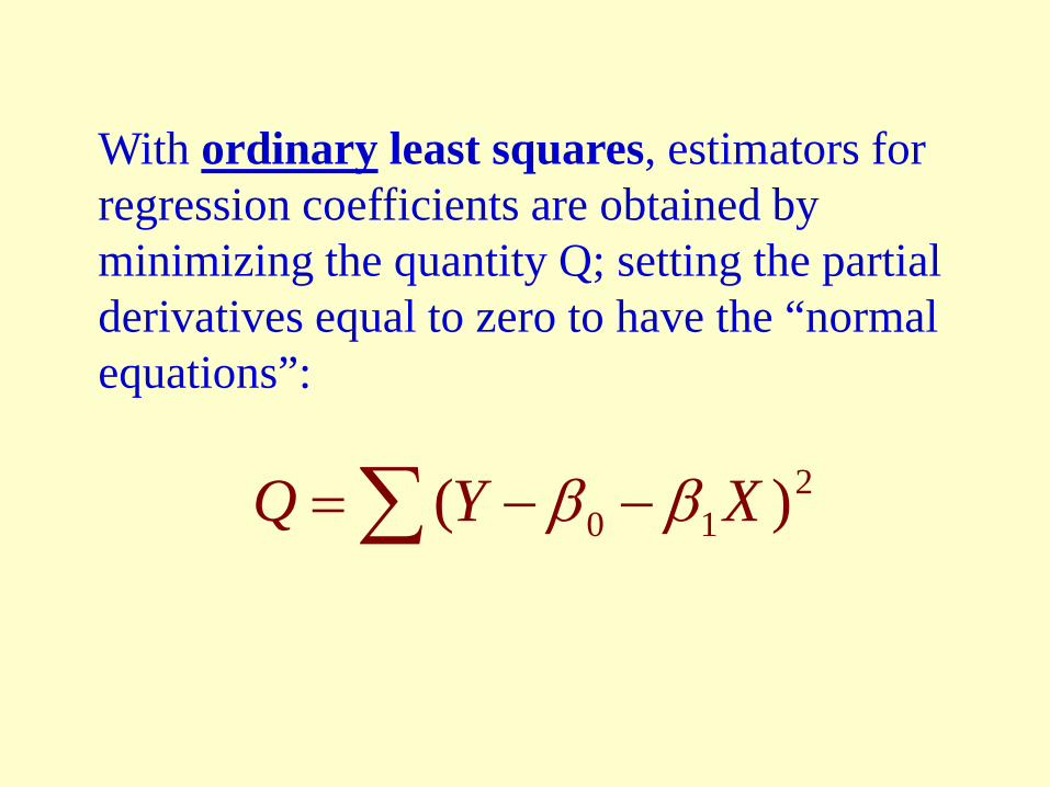
With ordinary least squares, estimators for regression coefficients are obtained by minimizing the quantity Q; setting the partial derivatives equal to zero to have the “normal equations”:

∑ −−= 210 )( XYQ ββ

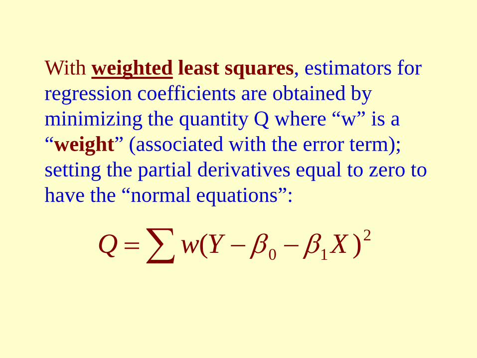
With weighted least squares, estimators for regression coefficients are obtained by minimizing the quantity Q where “w” is a “weight” (associated with the error term); setting the partial derivatives equal to zero to have the “normal equations”:

∑ −−= 210 )( XYwQ ββ

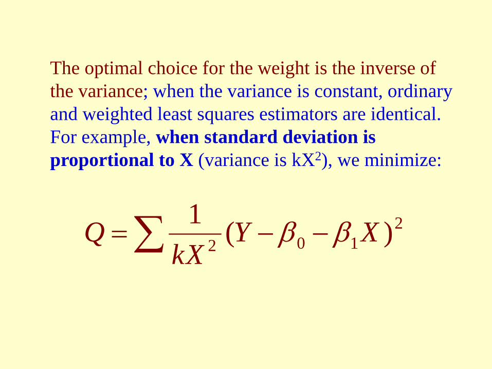
The optimal choice for the weight is the inverse of the variance; when the variance is constant, ordinary and weighted least squares estimators are identical. For example, when standard deviation is proportional to X (variance is kX2), we minimize:

∑ −−= 2102 )(1 XY

kXQ ββ

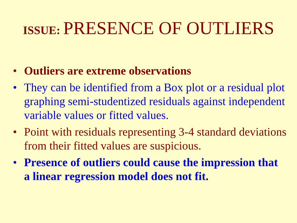
ISSUE: PRESENCE OF OUTLIERS

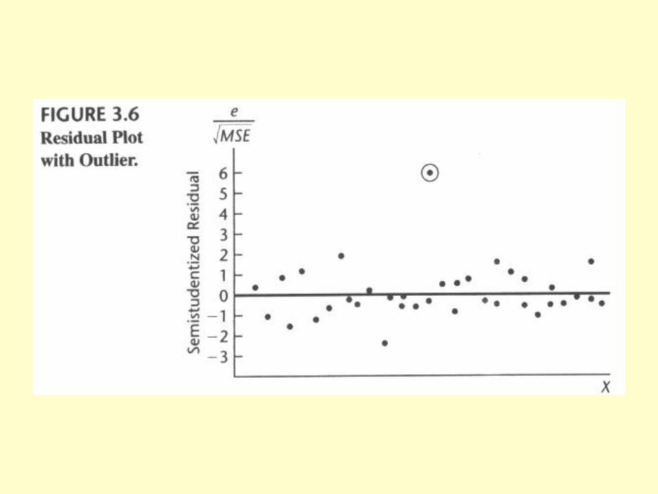
• Outliers are extreme observations • They can be identified from a Box plot or a residual plot

graphing semi-studentized residuals against independent variable values or fitted values.

• Point with residuals representing 3-4 standard deviations from their fitted values are suspicious.

• Presence of outliers could cause the impression that a linear regression model does not fit.

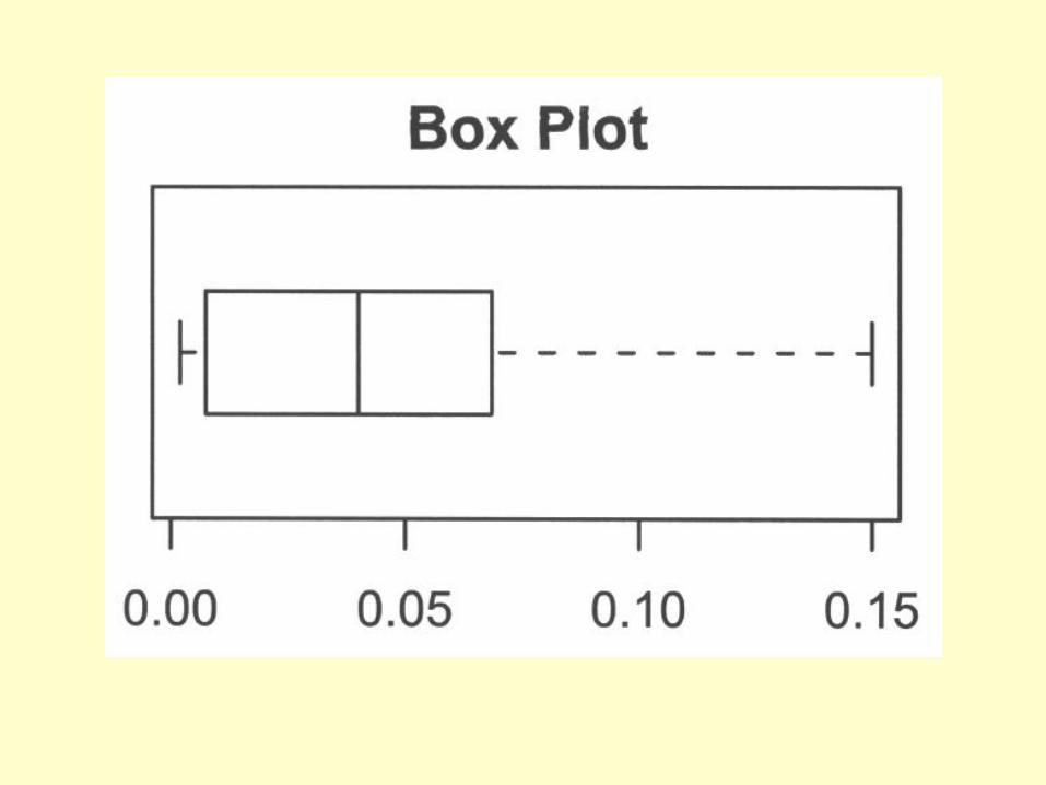
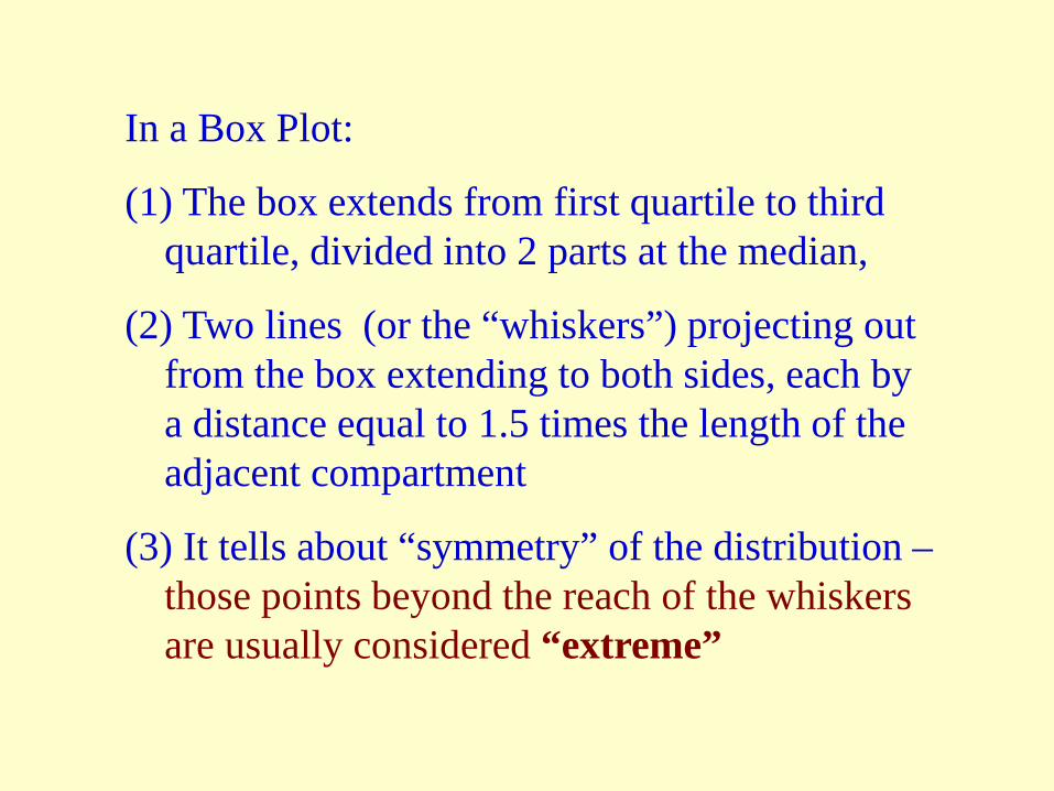
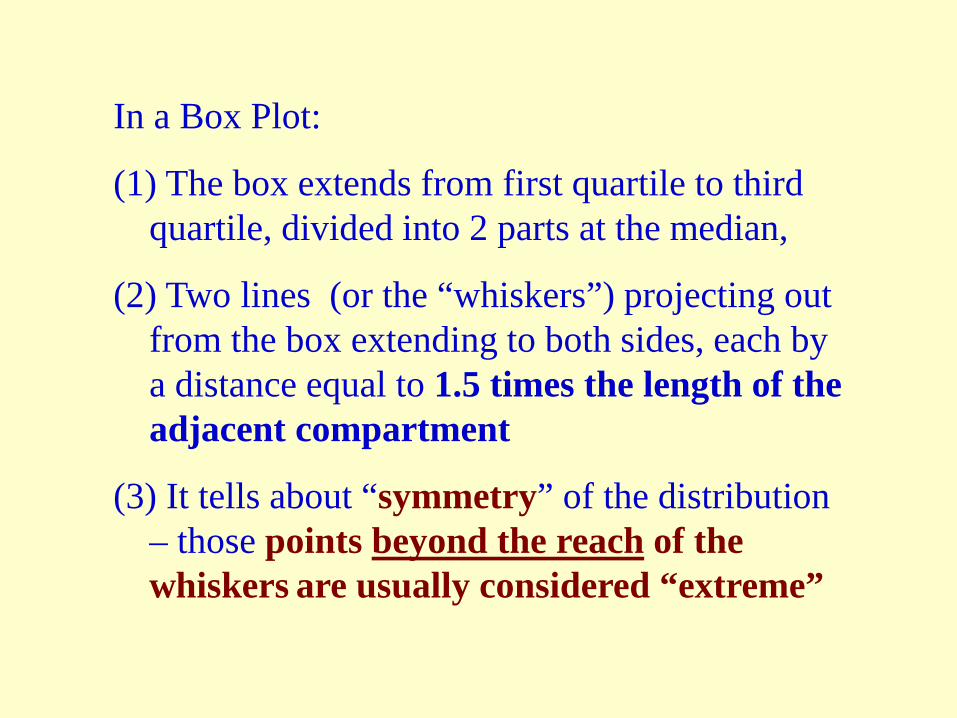
In a Box Plot:

(1) The box extends from first quartile to third quartile, divided into 2 parts at the median,

(2) Two lines (or the “whiskers”) projecting out from the box extending to both sides, each by a distance equal to 1.5 times the length of the adjacent compartment

(3) It tells about “symmetry” of the distribution – those points beyond the reach of the whiskers

are usually considered “extreme”

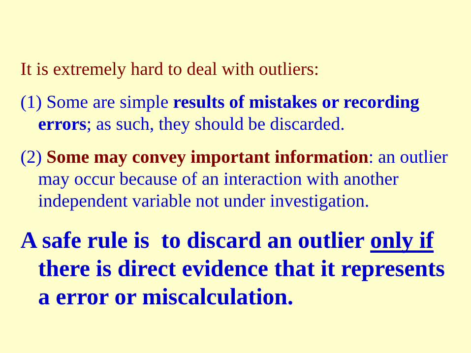
It is extremely hard to deal with outliers:

(1) Some are simple results of mistakes or recording errors; as such, they should be discarded.

(2) Some may convey important information: an outlier may occur because of an interaction with another independent variable not under investigation.

A safe rule is to discard an outlier only if there is direct evidence that it represents a error or miscalculation.

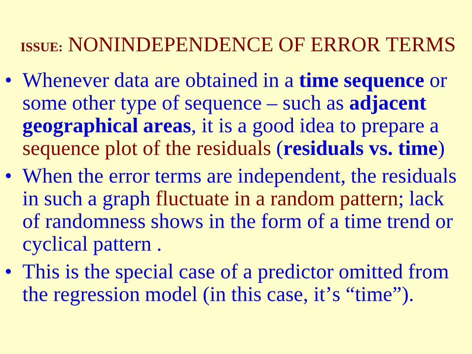
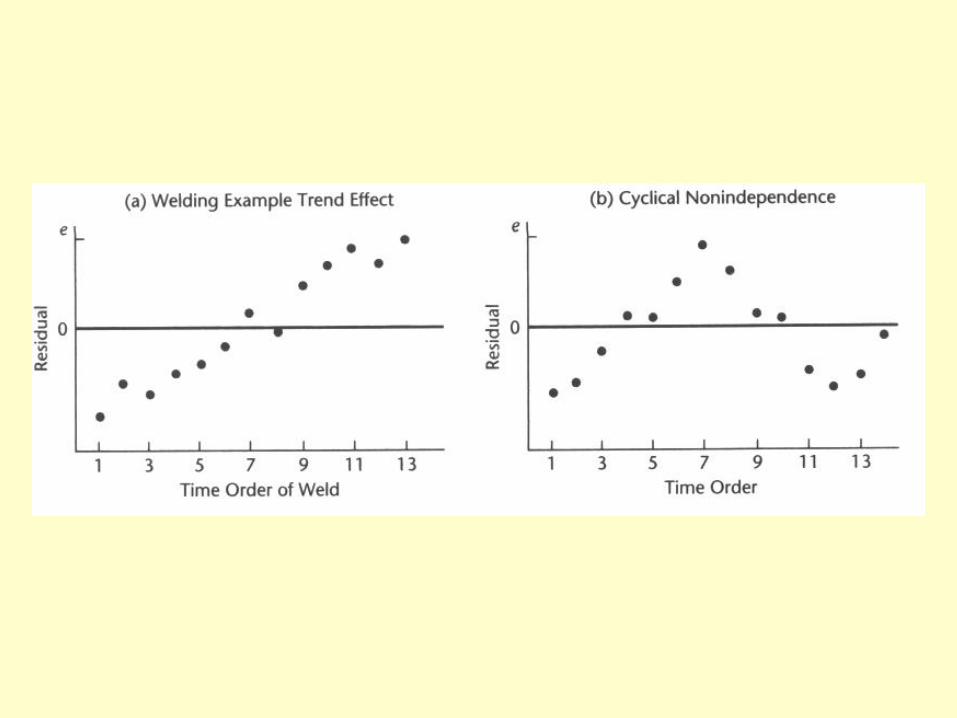
ISSUE: NONINDEPENDENCE OF ERROR TERMS

• Whenever data are obtained in a time sequence or some other type of sequence – such as adjacent geographical areas, it is a good idea to prepare a sequence plot of the residuals (residuals vs. time)

• When the error terms are independent, the residuals in such a graph fluctuate in a random pattern; lack of randomness shows in the form of a time trend or cyclical pattern .

• This is the special case of a predictor omitted from the regression model (in this case, it’s “time”).

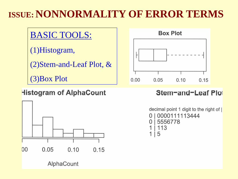
BASIC TOOLS: (1)Histogram,

(2)Stem-and-Leaf Plot, &

(3)Box Plot

ISSUE: NONNORMALITY OF ERROR TERMS

In a Box Plot:

(1) The box extends from first quartile to third quartile, divided into 2 parts at the median,

(2) Two lines (or the “whiskers”) projecting out from the box extending to both sides, each by a distance equal to 1.5 times the length of the adjacent compartment

(3) It tells about “symmetry” of the distribution – those points beyond the reach of the whiskers are usually considered “extreme”

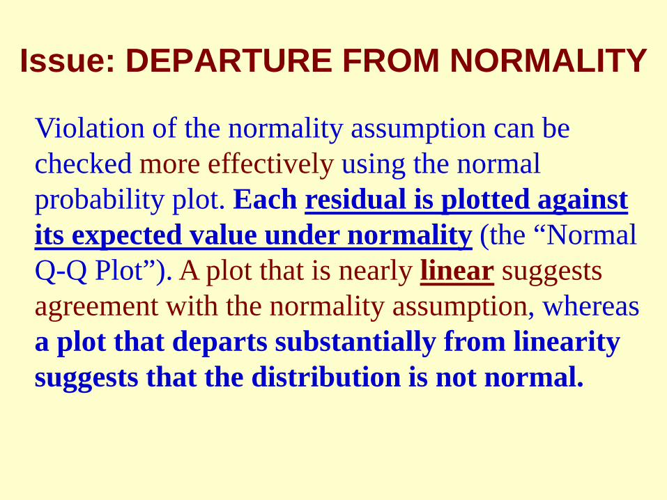
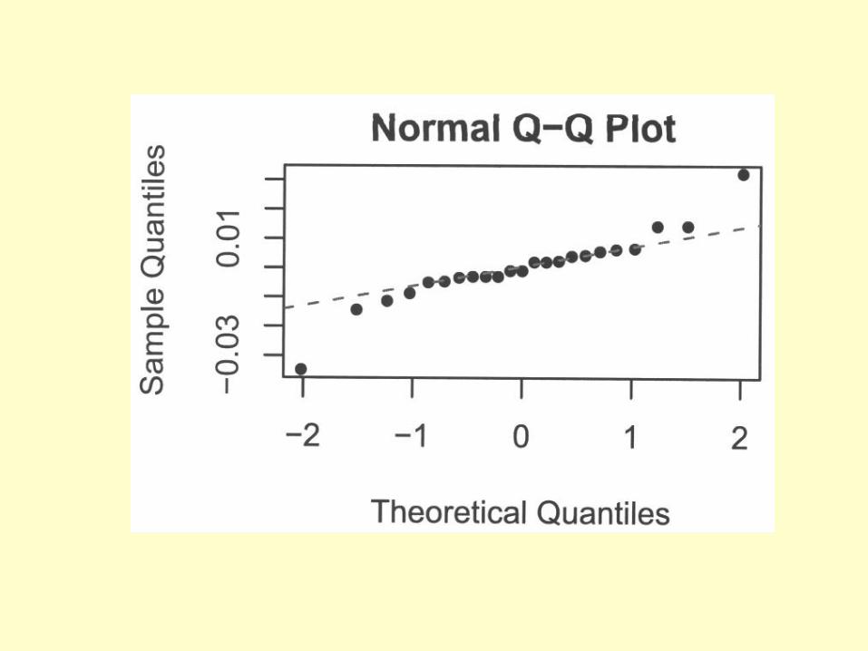
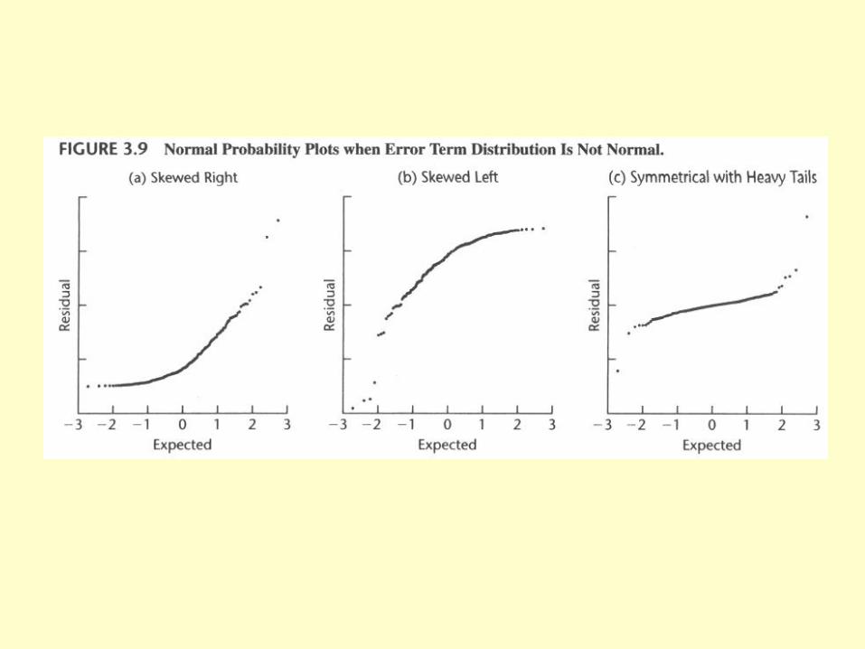
Issue: DEPARTURE FROM NORMALITY

Violation of the normality assumption can be checked more effectively using the normal probability plot. Each residual is plotted against its expected value under normality (the “Normal Q-Q Plot”). A plot that is nearly linear suggests agreement with the normality assumption, whereas a plot that departs substantially from linearity suggests that the distribution is not normal.

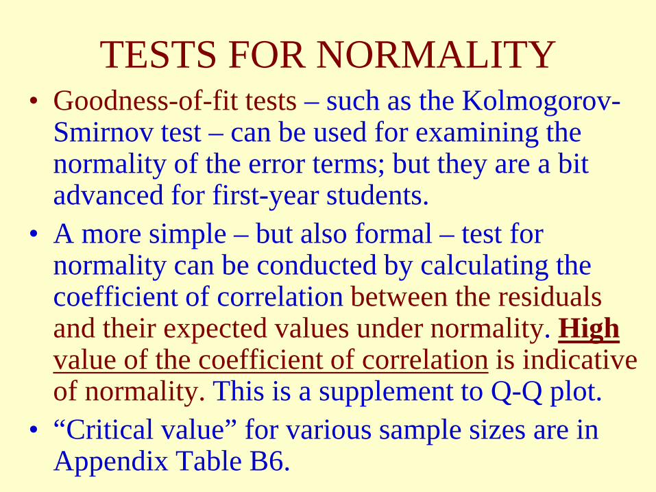
TESTS FOR NORMALITY • Goodness-of-fit tests – such as the Kolmogorov-

Smirnov test – can be used for examining the normality of the error terms; but they are a bit advanced for first-year students.

• A more simple – but also formal – test for normality can be conducted by calculating the coefficient of correlation between the residuals and their expected values under normality. High value of the coefficient of correlation is indicative of normality. This is a supplement to Q-Q plot.

• “Critical value” for various sample sizes are in Appendix Table B6.

When the distribution (of the response) is only near normal, most of the dots (on the Q-Q plot” are already very close to a straight line; the “cut-point” for rejection is quite high. Again, as mentioned, a formal statistical test may not really be needed here; but could use to supplement the Q-Q plot – more valuable when sample size n is small.

LotSize WorkHours80 39930 12150 22190 37670 36160 224

120 54680 352

100 35350 15740 16070 25290 38920 113

110 435100 42030 21250 26890 377

110 42130 27390 46840 24480 34270 323

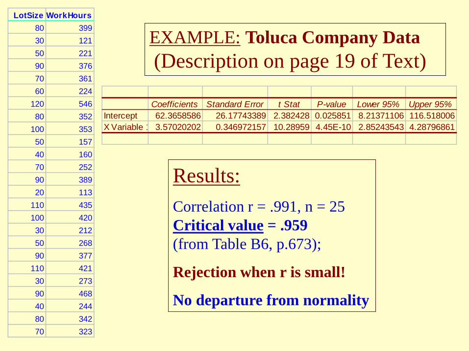
EXAMPLE: Toluca Company Data (Description on page 19 of Text)

Coefficients Standard Error t Stat P-value Lower 95% Upper 95%Intercept 62.3658586 26.17743389 2.382428 0.025851 8.21371106 116.518006X Variable 1 3.57020202 0.346972157 10.28959 4.45E-10 2.85243543 4.28796861

Results: Correlation r = .991, n = 25 Critical value = .959 (from Table B6, p.673);

Rejection when r is small!

No departure from normality

If the probability distributions of Y are not exactly normal but do not depart seriously, the sampling distributions of b0 and b1 would still be approximately normal with very little effects on the level of significance of the t-test for independence and the coverage of the confidence intervals. Even if the probability distributions of Y are far from normal, the effects are still minimal provided that the samples sizes are sufficiently large; i.e. the sampling distributions of b0 and b1 are asymptotically normal.

OMISSION OF OTHER PREDICTORS

Residuals should also be plotted against other potential independent variables – one at a time. “Time” was an earlier example in a sequential plot. If the factor under investigation is not related to the dependent and the independent variable, one would have a horizontal band of dots centered around zero which has special clustering pattern. If it is related to either the dependent or the independent variable then we would have a graph showing the residuals departing from zeros in a systematic fashion.

This is starting step in forming multiple regression models.

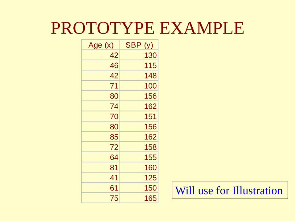
PROTOTYPE EXAMPLE Age (x) SBP (y)

42 13046 11542 14871 10080 15674 16270 15180 15685 16272 15864 15581 16041 12561 15075 165

Will use for Illustration

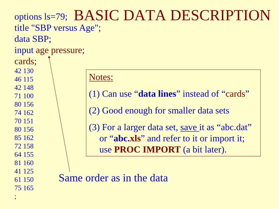
BASIC DATA DESCRIPTION options ls=79; title "SBP versus Age"; data SBP; input age pressure; cards; 42 130 46 115 42 148 71 100 80 156 74 162 70 151 80 156 85 162 72 158 64 155 81 160 41 125 61 150 75 165 ;

Notes:

(1) Can use “data lines” instead of “cards”

(2) Good enough for smaller data sets

(3) For a larger data set, save it as “abc.dat” or “abc.xls” and refer to it or import it; use PROC IMPORT (a bit later).

Same order as in the data

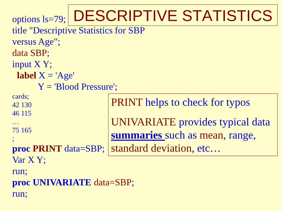
DESCRIPTIVE STATISTICS options ls=79; title "Descriptive Statistics for SBP versus Age"; data SBP; input X Y; label X = 'Age' Y = 'Blood Pressure'; cards; 42 130 46 115 … 75 165 ; proc PRINT data=SBP; Var X Y; run; proc UNIVARIATE data=SBP; run;

PRINT helps to check for typos

UNIVARIATE provides typical data summaries such as mean, range, standard deviation, etc…

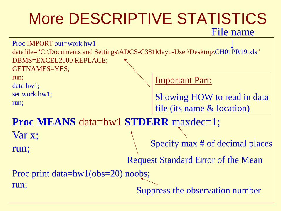
More DESCRIPTIVE STATISTICS Proc IMPORT out=work.hw1 datafile="C:\Documents and Settings\ADCS-C381Mayo-User\Desktop\CH01PR19.xls" DBMS=EXCEL2000 REPLACE; GETNAMES=YES; run; data hw1; set work.hw1; run;

Proc MEANS data=hw1 STDERR maxdec=1; Var x; run; Proc print data=hw1(obs=20) noobs; run;

Important Part:

Showing HOW to read in data file (its name & location)

Specify max # of decimal places

Suppress the observation number

Request Standard Error of the Mean

File name

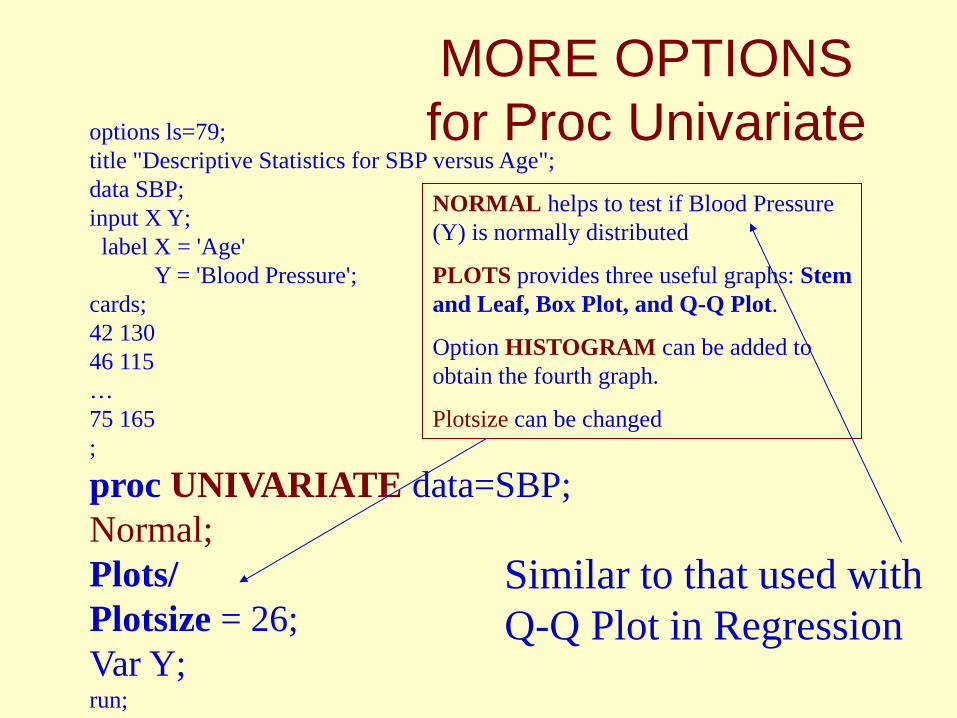
MORE OPTIONS for Proc Univariate options ls=79;

title "Descriptive Statistics for SBP versus Age"; data SBP; input X Y; label X = 'Age' Y = 'Blood Pressure'; cards; 42 130 46 115 … 75 165 ;

proc UNIVARIATE data=SBP; Normal; Plots/ Plotsize = 26; Var Y; run;

NORMAL helps to test if Blood Pressure (Y) is normally distributed

PLOTS provides three useful graphs: Stem and Leaf, Box Plot, and Q-Q Plot.

Option HISTOGRAM can be added to obtain the fourth graph.

Plotsize can be changed

Similar to that used with Q-Q Plot in Regression

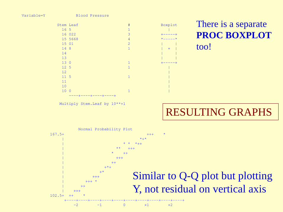
Variable=Y Blood Pressure Stem Leaf # Boxplot 16 5 1 | 16 022 3 +-----+ 15 5668 4 *-----* 15 01 2 | | 14 8 1 | + | 14 | | 13 | | 13 0 1 +-----+ 12 5 1 | 12 | 11 5 1 | 11 | 10 | 10 0 1 | ----+----+----+----+

Multiply Stem.Leaf by 10**+1 Normal Probability Plot 167.5+ +++ * | *+* | * * *++ | ** +++ | * ++ | +++ | ++ | +*+ | +* | +++ | +++ * | ++ | +++ 102.5+ ++ * +----+----+----+----+----+----+----+----+----+----+ -2 -1 0 +1 +2

RESULTING GRAPHS

Similar to Q-Q plot but plotting Y, not residual on vertical axis

There is a separate PROC BOXPLOT too!

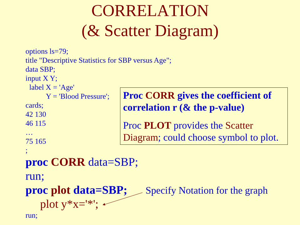
CORRELATION (& Scatter Diagram)

options ls=79; title "Descriptive Statistics for SBP versus Age"; data SBP; input X Y; label X = 'Age' Y = 'Blood Pressure'; cards; 42 130 46 115 … 75 165 ;

proc CORR data=SBP; run; proc plot data=SBP; plot y*x='*'; run;

Proc CORR gives the coefficient of correlation r (& the p-value)

Proc PLOT provides the Scatter Diagram; could choose symbol to plot.

Specify Notation for the graph

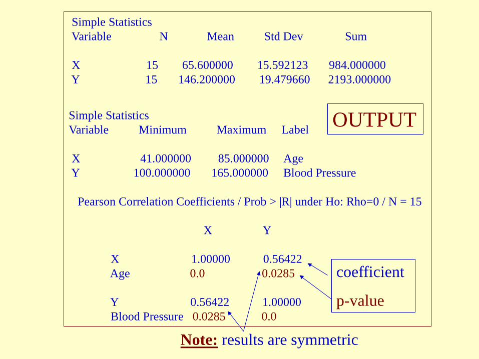
Simple Statistics Variable N Mean Std Dev Sum X 15 65.600000 15.592123 984.000000 Y 15 146.200000 19.479660 2193.000000

Simple Statistics Variable Minimum Maximum Label X 41.000000 85.000000 Age Y 100.000000 165.000000 Blood Pressure Pearson Correlation Coefficients / Prob > |R| under Ho: Rho=0 / N = 15 X Y X 1.00000 0.56422 Age 0.0 0.0285 Y 0.56422 1.00000 Blood Pressure 0.0285 0.0

coefficient

p-value

Note: results are symmetric

OUTPUT

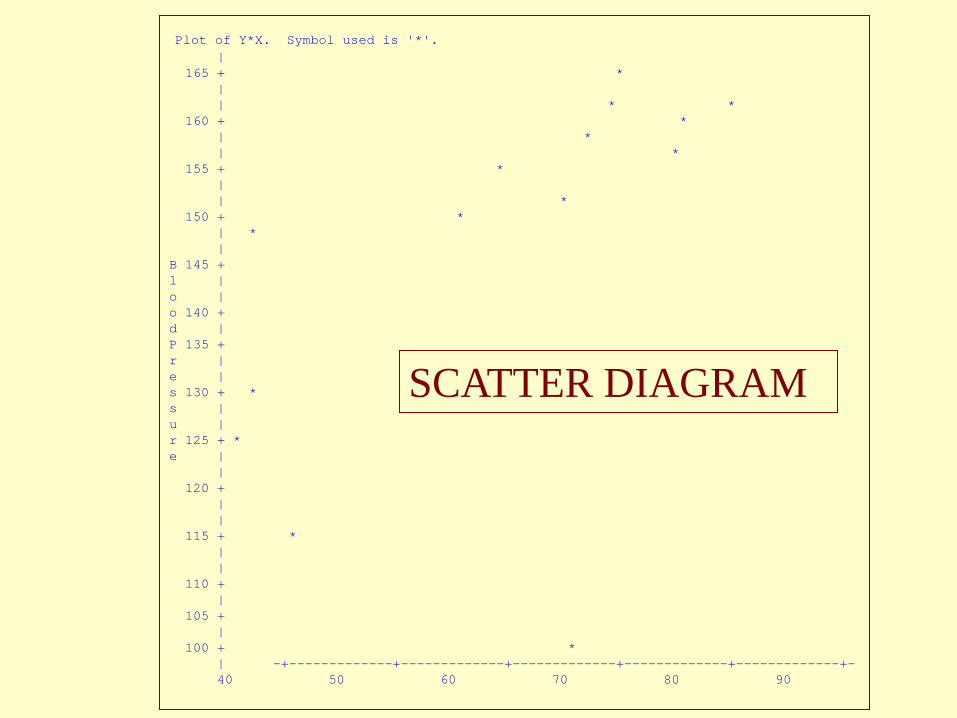
Plot of Y*X. Symbol used is '*'. | 165 + * | | * * 160 + * | * | * 155 + * | | * 150 + * | * | B 145 + l | o | o 140 + d | P 135 + r | e | s 130 + * s | u | r 125 + * e | | 120 + | | 115 + * | | 110 + | 105 + | 100 + * | -+-------------+-------------+-------------+-------------+-------------+- 40 50 60 70 80 90

SCATTER DIAGRAM

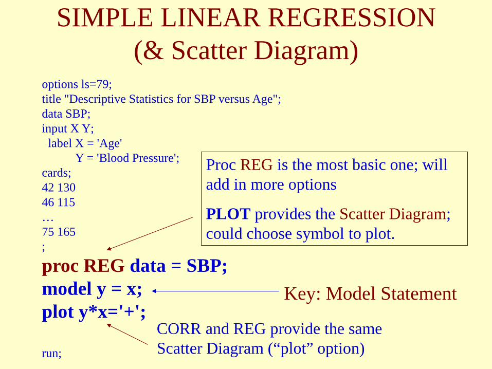
SIMPLE LINEAR REGRESSION (& Scatter Diagram)

options ls=79; title "Descriptive Statistics for SBP versus Age"; data SBP; input X Y; label X = 'Age' Y = 'Blood Pressure'; cards; 42 130 46 115 … 75 165 ;

proc REG data = SBP; model y = x; plot y*x='+'; run;

Proc REG is the most basic one; will add in more options

PLOT provides the Scatter Diagram; could choose symbol to plot.

CORR and REG provide the same Scatter Diagram (“plot” option)

Key: Model Statement

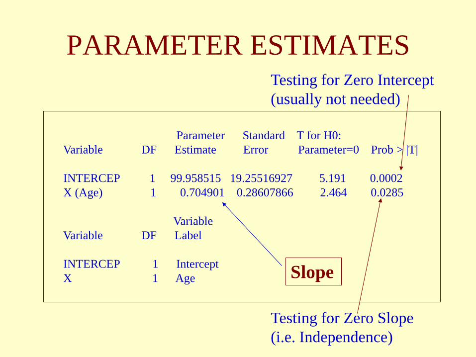
Parameter Standard T for H0: Variable DF Estimate Error Parameter=0 Prob > |T| INTERCEP 1 99.958515 19.25516927 5.191 0.0002 X (Age) 1 0.704901 0.28607866 2.464 0.0285 Variable Variable DF Label INTERCEP 1 Intercept X 1 Age

PARAMETER ESTIMATES

Slope

Testing for Zero Slope (i.e. Independence)

Testing for Zero Intercept (usually not needed)

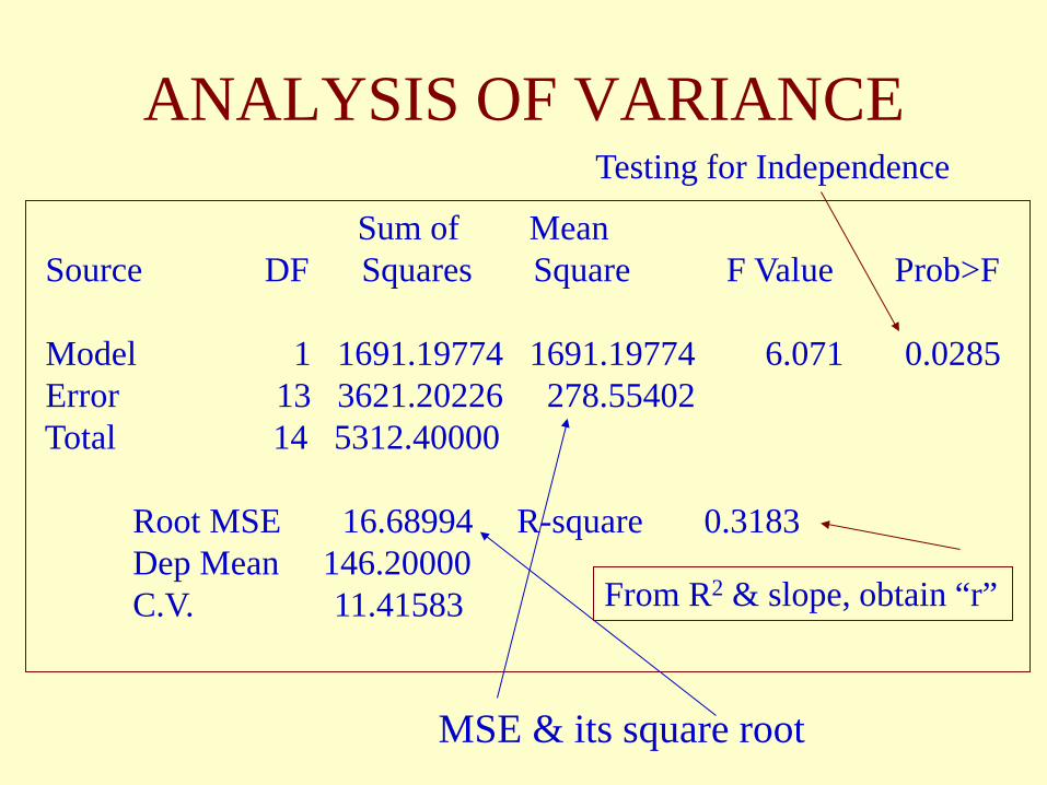
ANALYSIS OF VARIANCE

Sum of Mean Source DF Squares Square F Value Prob>F Model 1 1691.19774 1691.19774 6.071 0.0285 Error 13 3621.20226 278.55402 Total 14 5312.40000 Root MSE 16.68994 R-square 0.3183 Dep Mean 146.20000 C.V. 11.41583

MSE & its square root

Testing for Independence

From R2 & slope, obtain “r”

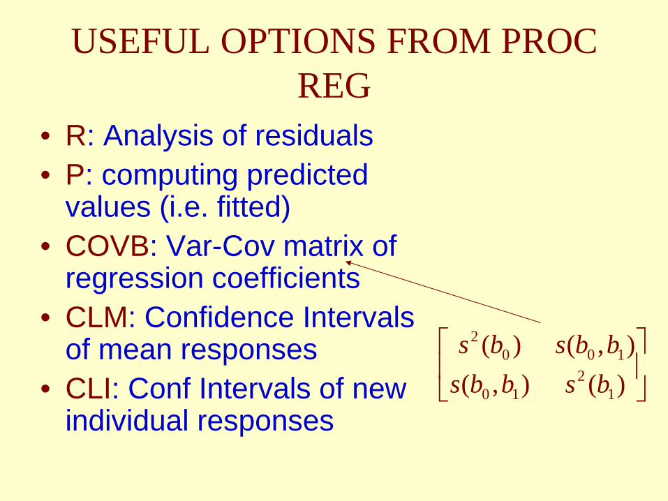
USEFUL OPTIONS FROM PROC REG

• R: Analysis of residuals • P: computing predicted

values (i.e. fitted) • COVB: Var-Cov matrix of

regression coefficients • CLM: Confidence Intervals

of mean responses • CLI: Conf Intervals of new

individual responses

)(),(),()(

12

10

1002

bsbbsbbsbs

ANALYSIS OF RESIDUALS

options ls=79; title "Descriptive Statistics for SBP versus Age"; data SBP; input X Y; label X = 'Age' Y = 'Blood Pressure'; cards; 42 130 … 75 165 ;

proc reg data = SBP noprint; model y = x/R; run;

This short program achieves the same thing and more; it helps to set up a Table just like TABLE 1.2 on page 22 of the text book and student residuals – plus all regression analysis results.

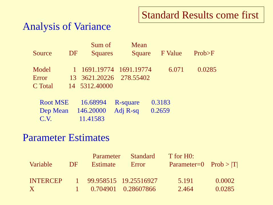
Analysis of Variance Sum of Mean Source DF Squares Square F Value Prob>F Model 1 1691.19774 1691.19774 6.071 0.0285 Error 13 3621.20226 278.55402 C Total 14 5312.40000 Root MSE 16.68994 R-square 0.3183 Dep Mean 146.20000 Adj R-sq 0.2659 C.V. 11.41583

Parameter Estimates Parameter Standard T for H0: Variable DF Estimate Error Parameter=0 Prob > |T| INTERCEP 1 99.958515 19.25516927 5.191 0.0002 X 1 0.704901 0.28607866 2.464 0.0285

Standard Results come first

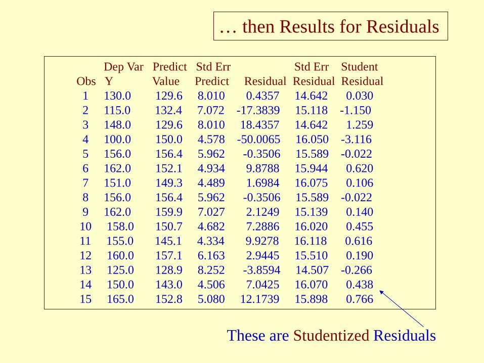
Dep Var Predict Std Err Std Err Student Obs Y Value Predict Residual Residual Residual 1 130.0 129.6 8.010 0.4357 14.642 0.030 2 115.0 132.4 7.072 -17.3839 15.118 -1.150 3 148.0 129.6 8.010 18.4357 14.642 1.259 4 100.0 150.0 4.578 -50.0065 16.050 -3.116 5 156.0 156.4 5.962 -0.3506 15.589 -0.022 6 162.0 152.1 4.934 9.8788 15.944 0.620 7 151.0 149.3 4.489 1.6984 16.075 0.106 8 156.0 156.4 5.962 -0.3506 15.589 -0.022 9 162.0 159.9 7.027 2.1249 15.139 0.140 10 158.0 150.7 4.682 7.2886 16.020 0.455 11 155.0 145.1 4.334 9.9278 16.118 0.616 12 160.0 157.1 6.163 2.9445 15.510 0.190 13 125.0 128.9 8.252 -3.8594 14.507 -0.266 14 150.0 143.0 4.506 7.0425 16.070 0.438 15 165.0 152.8 5.080 12.1739 15.898 0.766

… then Results for Residuals

These are Studentized Residuals

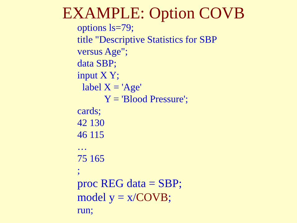
EXAMPLE: Option COVB options ls=79; title "Descriptive Statistics for SBP versus Age"; data SBP; input X Y; label X = 'Age' Y = 'Blood Pressure'; cards; 42 130 46 115 … 75 165 ; proc REG data = SBP; model y = x/COVB; run;

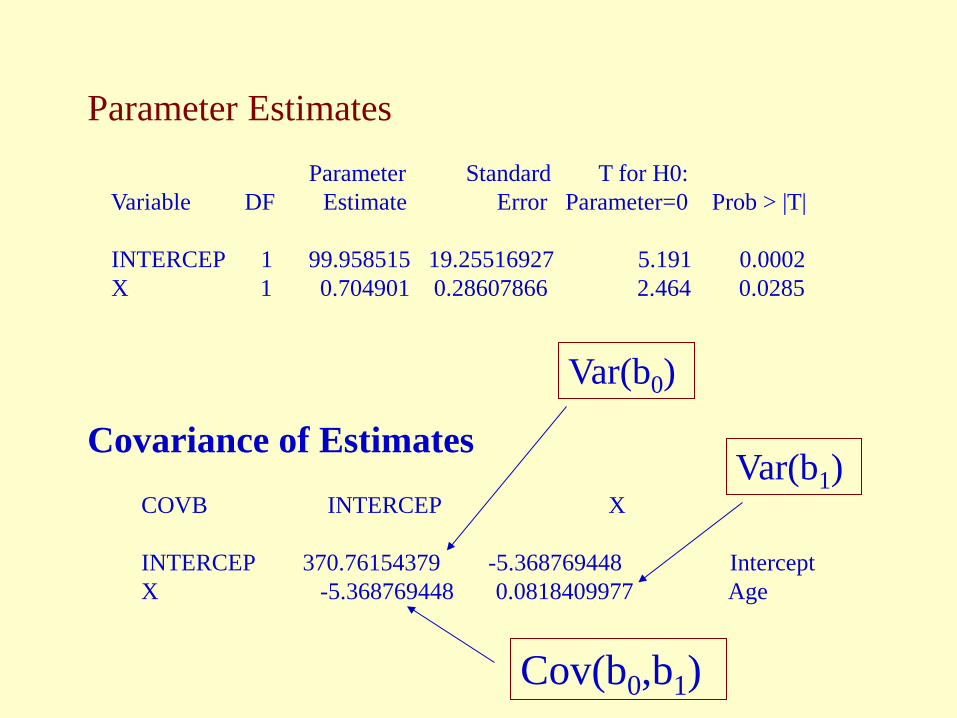
Parameter Estimates Parameter Standard T for H0: Variable DF Estimate Error Parameter=0 Prob > |T| INTERCEP 1 99.958515 19.25516927 5.191 0.0002 X 1 0.704901 0.28607866 2.464 0.0285

Covariance of Estimates COVB INTERCEP X INTERCEP 370.76154379 -5.368769448 Intercept X -5.368769448 0.0818409977 Age

Var(b0)

Var(b1)

Cov(b0,b1)

EXAMPLE: Option CLM options ls=79; title "Descriptive Statistics for SBP versus Age"; data SBP; input X Y; label X = 'Age' Y = 'Blood Pressure'; cards; 42 130 46 115 … 75 165 ; proc REG data = SBP; model y = x/CLM; run;

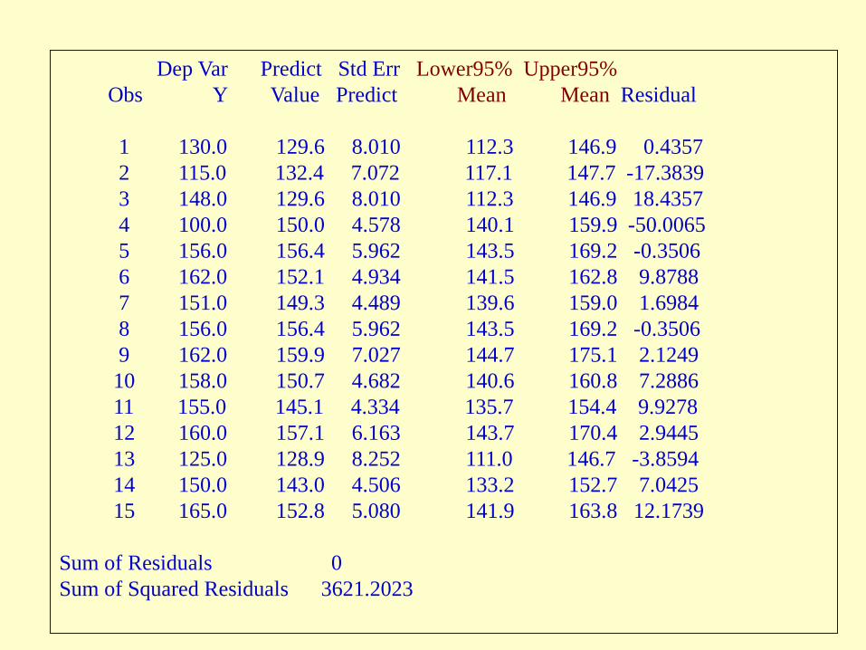
Dep Var Predict Std Err Lower95% Upper95% Obs Y Value Predict Mean Mean Residual 1 130.0 129.6 8.010 112.3 146.9 0.4357 2 115.0 132.4 7.072 117.1 147.7 -17.3839 3 148.0 129.6 8.010 112.3 146.9 18.4357 4 100.0 150.0 4.578 140.1 159.9 -50.0065 5 156.0 156.4 5.962 143.5 169.2 -0.3506 6 162.0 152.1 4.934 141.5 162.8 9.8788 7 151.0 149.3 4.489 139.6 159.0 1.6984 8 156.0 156.4 5.962 143.5 169.2 -0.3506 9 162.0 159.9 7.027 144.7 175.1 2.1249 10 158.0 150.7 4.682 140.6 160.8 7.2886 11 155.0 145.1 4.334 135.7 154.4 9.9278 12 160.0 157.1 6.163 143.7 170.4 2.9445 13 125.0 128.9 8.252 111.0 146.7 -3.8594 14 150.0 143.0 4.506 133.2 152.7 7.0425 15 165.0 152.8 5.080 141.9 163.8 12.1739 Sum of Residuals 0 Sum of Squared Residuals 3621.2023

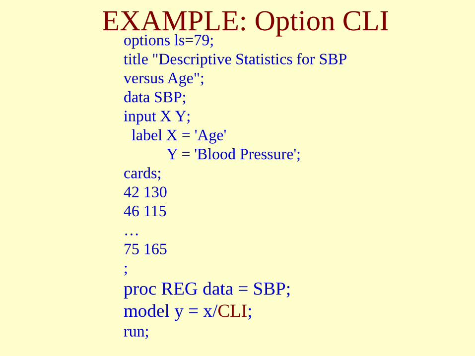
EXAMPLE: Option CLI options ls=79; title "Descriptive Statistics for SBP versus Age"; data SBP; input X Y; label X = 'Age' Y = 'Blood Pressure'; cards; 42 130 46 115 … 75 165 ; proc REG data = SBP; model y = x/CLI; run;

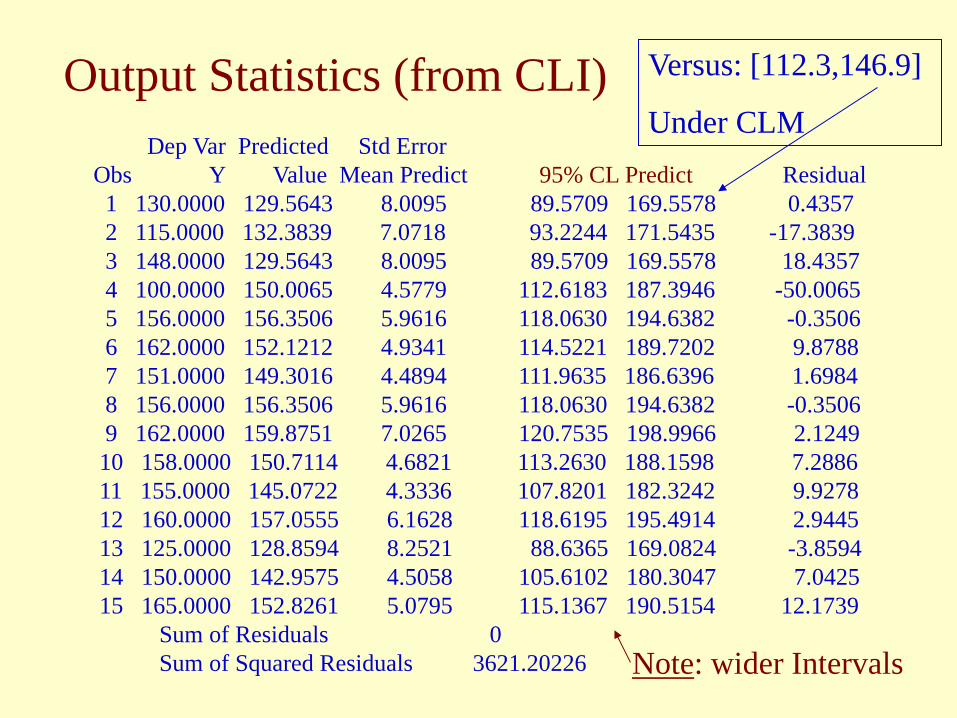
Output Statistics (from CLI) Dep Var Predicted Std Error Obs Y Value Mean Predict 95% CL Predict Residual 1 130.0000 129.5643 8.0095 89.5709 169.5578 0.4357 2 115.0000 132.3839 7.0718 93.2244 171.5435 -17.3839 3 148.0000 129.5643 8.0095 89.5709 169.5578 18.4357 4 100.0000 150.0065 4.5779 112.6183 187.3946 -50.0065 5 156.0000 156.3506 5.9616 118.0630 194.6382 -0.3506 6 162.0000 152.1212 4.9341 114.5221 189.7202 9.8788 7 151.0000 149.3016 4.4894 111.9635 186.6396 1.6984 8 156.0000 156.3506 5.9616 118.0630 194.6382 -0.3506 9 162.0000 159.8751 7.0265 120.7535 198.9966 2.1249 10 158.0000 150.7114 4.6821 113.2630 188.1598 7.2886 11 155.0000 145.0722 4.3336 107.8201 182.3242 9.9278 12 160.0000 157.0555 6.1628 118.6195 195.4914 2.9445 13 125.0000 128.8594 8.2521 88.6365 169.0824 -3.8594 14 150.0000 142.9575 4.5058 105.6102 180.3047 7.0425 15 165.0000 152.8261 5.0795 115.1367 190.5154 12.1739 Sum of Residuals 0 Sum of Squared Residuals 3621.20226 Note: wider Intervals

Versus: [112.3,146.9]

Under CLM

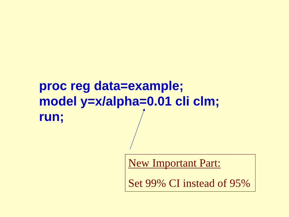
proc reg data=example; model y=x/alpha=0.01 cli clm; run;

New Important Part:

Set 99% CI instead of 95%

Readings & Exercises • Readings: A thorough reading of the text’s

sections 3.1-3.3 (pp. 100-114) and 3.5-3.7 (pp. 115-127) is highly recommended.

• Exercises: The following exercises are good for practice, all from chapter 3 of text: 3.3, 3.7, 3.8, 3.9, 3.10, 3.11, and 3.18.

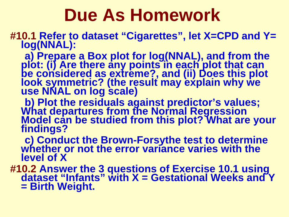
Due As Homework #10.1 Refer to dataset “Cigarettes”, let X=CPD and Y=

log(NNAL): a) Prepare a Box plot for log(NNAL), and from the

plot: (i) Are there any points in each plot that can be considered as extreme?, and (ii) Does this plot look symmetric? (the result may explain why we use NNAL on log scale)

b) Plot the residuals against predictor’s values; What departures from the Normal Regression Model can be studied from this plot? What are your findings?

c) Conduct the Brown-Forsythe test to determine whether or not the error variance varies with the level of X

#10.2 Answer the 3 questions of Exercise 10.1 using dataset “Infants” with X = Gestational Weeks and Y = Birth Weight.