Two-parameter Sample Path Large Deviations for Infinite Server

Queues

Blanchet, J., Chen, X., and Lam, H.

November 8, 2018

Abstract

Let Qλ (t, y) be the number of people present at time t with y units of remaining service timein an infinite server system with arrival rate equal to λ > 0. In the presence of a non-latticerenewal arrival process and assuming that the service times have a continuous distribution,we obtain a large deviations principle for Qλ (·) /λ under the topology of uniform convergenceon [0, T ] × [0,∞). We illustrate our results by obtaining the most likely path, represented asa surface, to ruin in life insurance portfolios, and also we obtain the most likely surfaces tooverflow in the setting of loss queues.

1 Introduction

The asymptotic analysis of queueing systems with many servers in heavy-traffic has received sub-stantial attention, especially in recent years. Among the earliest references that come to mindin connection to this topic is the work of [7] on heavy-traffic limits for the infinite-server queue.Another highly influential paper in the area is [6] in the context of many server Markovian queues,which introduced a scaling that is now known as the “Quality and Efficiency Driven” regime. Theideas in these papers have fueled more recent results in the asymptotic analysis of many serversystems such as: [12], [8], [13], [9], [10], in the setting of many server queues, and [5], [2], [11], [14],in the setting of the infinite server queue. The asymptotic analysis of queueing systems with manyservers has been motivated by applications in service engineering, in particular in the context ofcall centers and health-care operations. Another set of application areas that is also very relevant,but that is infrequently mentioned in the analysis of many server systems is that of insurance math-ematics. It is clear, for instance, that a portfolio of insurance policies can be directly modeled asan infinite server system; casting insurance portfolios in this framework is particularly appealing inthe setting of life insurance as we shall illustrate in Section 5.

So far most of the asymptotic analysis of many server systems has concentrated mainly onfluid and heavy-traffic approximations. Meanwhile, the literature on large deviations analysis formany server queues is not as extensive as that of fluid or diffusion approximations; despite the factthat it is clearly of interest to understand the large deviations behavior of these types of systems.For instance, consider the consequences of dropping calls in an emergency call center or beingunable to satisfy the demand for critically ill patients in the context of health-care applications.In the insurance setting, for instance, it is of interest to estimate ruin probabilities and, perhapseven more importantly, understanding the most likely path (or set of paths) to ruin. Risk theorytypically concentrates on ruin probabilities for aggregated models, such as the classical ruin model

1

arX

iv:1

207.

5164

v1 [

mat

h.PR

] 2

1 Ju

l 201

2

2

(see [1]); the results in this paper, as we shall illustrate, provide a systematic way for assessing ruinprobabilities for a class of bottom-up models.

Our main contribution in this paper is to provide the first sample-path large deviations analysisof the state descriptor of the infinite server queueing model in heavy-traffic (i.e. as the arrivalrate increases to infinity without introducing any scaling on the service times). The statement ofour main result, which is given in Theorem 1, features a convenient representation of a good largedeviations rate function, under a strong topology, that later we use in some applied settings ofinterest. For instance, we compute the most likely path to overflow in a loss system, and also themost likely path to ruin for a life insurance portfolio that embeds an infinite server queue with aparticular service cost structure. It is important to emphasize that our results take advantage of aconvenient representation of the system’s description that facilitates the representation of the ratefunction; detailed discussion on this system’s representation is given in Section 2.1. Previous largedeviations analysis of the infinite server queue has concentrated on queue-length characteristicsonly; see, for instance, [4] who develops large deviations for marginal quantities in the case ofrenewal arrivals, and [15] who develops sample path large deviations for the queue length processof infinite server queues in tandem in the case of Poisson arrivals.

Our large deviations analysis complement results on fluid analysis and diffusion approximationsrecently obtained for infinite server systems. For example, [11] have shown that the state descriptorof the infinite server queue, suitably parameterized in terms of a two-parameter stochastic process,converges after centering and re-scaling to a Gaussian process; see also [14] who interpret the statedescriptor of the infinite server queue as a measure valued process acting on the space of tempereddistributions. These recent results, in turn, extend prior work by [5] in the context of discrete andbounded service time distributions, and [2] for the case of Poisson arrivals.

The analysis of the infinite server queue is important as it serves as a building block for othermodels of interest. For instance, in the setting of loss models one can clearly couple the losssystems with associated infinite server systems, and in the setting of many server queues [13] showshow one can precisely understand queues with multiple servers as a perturbation of infinite serverqueues. Furthermore, the infinite server model is a classical model in queueing theory that servesas direct model in important applications. Of particular interest to us, as mentioned earlier, arethe applications to insurance mathematics.

The rest of the paper is organized as follows. In Section 2 we introduce our problem settingand provide a statement of our main result. This is a fundamental section and it is divided intothree parts. We first shall introduce our assumptions and define our notation. Then we providethe precise mathematical statement of our result, and, finally, we will provide a heuristic argumentthat allows us to gain some intuition behind our main result. The next two sections then providethe proof of our main result. We first show our result for bounded service times in Section 3. Then,in Section 4, we apply a truncation argument to extend our result to unbounded service times.Finally, in Section 5 we apply our result to computing the most likely paths to rare events in thesetting of loss queueing systems and also in the setting of ruin probabilities for large life insuranceportfolios.

2 Assumptions, Notation, and Main Result

The purpose of this section is threefold. First we shall clearly state our assumptions and introducenecessary notation for our development. Second, we shall explain the main large deviations resultand provide a heuristic derivation of the rate function that we obtain. Finally, we shall provide a

3

road map for the strategy behind the proof which will be presented in subsequent sections.

2.1 Assumptions and Notation

We shall describe an underlying system corresponding to an arrival rate λ. We call the system withλ = 1, i.e. one customer per unit time, our “base system”; eventually we shall send λ to infinity inour asymptotic analysis. We collect our assumptions as follows.

Assumptions and notation concerning the arrival process. For the base system, we assumethe interarrival times are non-lattice, i.i.d., positive random variables (Un : n ≥ 1) with finiteexponential moments in a neighborhood of the origin; in precise words, κ(θ) := logEeθUn <∞ forsome θ > 0. In our λ-scaled system, the arrivals come λ times faster (i.e. the n-th interarrivaltimes becomes Un/λ). The associated logarithmic moment generating of the λ-scaled service timesis then κλ(θ) := logEeθUn/λ = κ(θ/λ) <∞ for some θ > 0.

The time at which the n-th arrival occurs in the base system is An = U1 + ... + Un for n ≥ 1.We simply define A0 := 0 and then let N (t) := max{n ≥ 0 : An ≤ t} be the number of arrivals thathave occurred up to time t in the base system. It is important to keep in mind that N (·) increasesby one unit at discontinuity points since we are assuming that the Un’s are positive.

Eventually, we shall increase the arrival rate, so it is sensible to define Nλ (t) := N (λt).Define the so-called infinitesimal logarithmic moment generating function for the arrival process

via ψN (θ) = −κ−1(−θ) (see [4]). This definition is motivated by the fact that

limt→∞

λ−1 logE exp (θ[Nλ (t+ δ)−Nλ (t)]) = ψN (θ) δ

for any δ > 0. Since the Un’s are positive with probability one we have that ψN (·) is continuousand strictly convex on the positive line. We also assume that ψN (·) is continuously differentiablethroughout R. This assumption is satisfied for most arrival processes, certainly for interarrivaltimes that are strictly positive and such that sup{κ (θ) : κ (θ) <∞} =∞.

Assumptions and notation concerning the service times. We assume that the n-th customerthat arrives to the base system (i.e. at time An) brings up a service requirement of size Vn. Thesequence (Vn : n ≥ 1) is assumed to be i.i.d. We write F (x) = P (Vn ≤ x) to denote the associateddistribution function evaluated at x, and set F (x) := 1−F (x) to be the tail distribution. Moreover,we assume that F (·) is continuous.

Two-parameter representation of system status. Let Qλ (t, y) denote the number of cus-tomers who arrived before or at time t and leave after time y in the λ-scaled system. In otherwords,

Qλ (t, y) = Qλ (0, y − t) +

Nλ(t)∑n=1

I (Vn +An/λ > y) .

We shall assume that the system is initially empty at the beginning. This is done for simplicity.Since we have infinitely many servers, we can incorporate the initial configuration by keeping trackof its evolution independently of what occurs subsequently. Given our assumption of an initialempty system we then have that Qλ (0, u) = 0 for all u ≥ 0. Note that for t ∈ [0, T ] and y ≥ 0,

Qλ (t, y) = Qλ (t ∧ y, y) +Nλ (t)−Nλ (t ∧ y) . (1)

4

It is worth comparing the current system representation with the more common one involvingthe quantity Qλ (t, u) defined as the number of customers in the system currently at time t whohave residual service time larger than u ≥ 0; more precisely, Qλ (t, u) = Qλ (t, u+ t). These twosystem representations are equivalent in the sense that (Qλ (t, u) : t ∈ [0, T ], u ≥ 0) encodes theevolution of the infinite server systems and thus, such evolution can be used in principle to retrieve(Qλ (t, u) : t ∈ [0, T ], u ≥ 0). We have chosen the representation based on Qλ to facilitate therepresentation of the rate function; a more detailed discussion is given towards the end of Section2.2.1. In addition, the representation based on Qλ allows to obtain a rich large deviations principleto which one can apply the contraction principle directly to several continuous functions of interest.For instance, it follows immediately that the arrival process Nλ (t) = Qλ (t, 0), and the departureprocess, Dλ (t) := Nλ (t) − Qλ (t, t) are continuous functions under the topology that we consider(and that we shall discuss in the next paragraphs). More applications of the contraction principlewill be discussed in Section 5.

Discussion about the topological space. Let D = {(t, y) : 0 ≤ t ≤ T, y ≥ 0} and let us write|| · ||C to denote the supremum norm over any set C. The space of functions that we consider for ourlarge deviations principle shall be denoted by L+,∞(D) and it corresponds to bounded functionswith domain in D, such that x (0, u) = 0 for u ≥ 0, x (t, ·) is non increasing, and x (t, ·) vanishesat infinity. We will develop the large deviations principle for the family of stochastic processes(Qλ/λ : λ > 0) on the space L+,∞(D) endowed with the topology generated by the supremumnorm. Following [3] p. 4, the probability measures in path space in our development are assumedto have been completed.

Our large deviations principle for Qλ/λ immediately implies in particular a large deviations prin-ciple in the Skorokhod topology in the space DDR[0,∞)[0, T ] which is the space of right-continuous-with-left-limits (RCLL) functions x, with domain on [0, T ], that take values on the space of RCLLfunctions taking values on R. That is, on each time point t in x = (x (t) : t ∈ [0, T ]) ∈ DDR[0,∞)[0, T ]is a function x (t) ∈ DR[0,∞). This is precisely the topology considered in [11], who also provide adiscussion on the benefits of using this topology relative to other natural (but weaker) alternativeoptions (see Section 2.3 in [11]).

An alternative approach that one might consider given the available results on functional weakconvergence analysis of the infinite server queue, such as [14], is to interpret the space descriptorof the infinite server queue as acting on the space of tempered distributions. We believe, however,that this approach, although elegant, has important limitations in terms of assumptions and theclass of functions to which the contraction principle can be directly applied to obtain other largedeviations principles of interest.

2.2 Statement of Our Main result.

We are now ready to state our main result. Let q := (q (t, y) : (t, y) ∈ D) ∈ L+,∞(D). We say thatq ∈ AC+ (D) if the following conditions hold:

i) q is absolutely continuous on D, and∫ ∞0

∫ ∞0

∣∣∣∣ ∂2

∂t ∂yq(t, y)

∣∣∣∣ dydt <∞,ii) ∂2q(t, y)/∂t ∂y = 0 almost everywhere for (t, y) ∈ {(t, y) : 0 ≤ y ≤ t ≤ T},iii) q (0, y) = 0 for y ≥ 0.If q ∈ AC+ (D), then we let I (q) be defined via

5

supθ(·,·)∈Cb[0,T ]×[0,∞)

∫ T

0

[∫ ∞t

θ(t, y − t)(− ∂2

∂t ∂yq(t, y)

)dy − ψN

(log

(∫ ∞0

eθ(t,y)dF (y)

))]dt (2)

where Cb[0, T ] × [0,∞) is the set of all bounded continuous functions on [0, T ] × [0,∞). On theother hand, if q ∈ L+,∞(D) fails to satisfy any of the conditions i) to iii), simply let I (q) =∞.

We now can state our main result.

Theorem 1. Under the set of assumptions discussed in Section 2.1, (Qλ/λ : λ > 0) satisfies a largedeviations principle with good rate function I (·) on the space (L+,∞(D), ||·||D). In precise terms,for each open set O we have that

limλ→∞ log1

λP (Qλ/λ ∈ O) ≥ − inf

q∈OI (q) ,

and for each closed set C

limλ→∞ log1

λP (Qλ/λ ∈ C) ≤ − inf

q∈CI (q) .

As an immediate corollary we obtain, as mentioned earlier, a large deviations principle for(Qλ/λ : λ > 0) under the Skorokhod topology in the space DDR[0,∞)[0, T ], discussed in the previoussection and introduced in [11].

We shall explain the strategy behind the proof of Theorem 1. First, we shall introduce anauxiliary continuous process, Qλ/λ, which shall be defined later in Section 2.3. We will showthat Qλ/λ is exponentially equivalent to Qλ/λ. Second, in addition to the assumptions imposedin Section 2.1 we will assume that there exists a deterministic constant M ∈ (0,∞) such thatP (Vn ∈ [0,M ]) = 1. In the third and last part of the argument we will relax this truncationassumption.

In turn, the first part of the argument (i.e. assuming truncation) is divided into several steps.The first step consists in developing the large deviations principle for Qλ/λ with rate I (·)

under the topology of pointwise convergence using the Dawson-Gartner projective limit theorem.The second step involves showing that Qλ/λ is exponentially tight as λ → ∞ under the uniformtopology on the compact set [0, T ] × [0,M ]. The third and last step involves lifting the largedeviations principle to the uniform topology.

During the second part we introduce an approximation scheme that proceeds by ignoring thecustomers that arrive to the system with a service time larger than K. Using a coupling argument,the process that is obtained using this scheme is shown to be a good approximation to the originalsystem for the purpose of computing large deviations probabilities.

However, before we do this let us provide a heuristic argument in order to guess the form of therate function. Later we will explain what are the technical difficulties that need to be addressed.

2.2.1 Guessing the Rate Function: A Heuristic Approach

One can take advantage of the point process representation of the input process (i.e. the arrivalsand the service times represented as a marked point process). Let us start with the case of Poissonarrivals. We shall briefly explain how to adapt the development that follows to the more generalcase of renewal arrivals.

6

Consider the scaled system with arrival rate λ and suppose that F (·) has a density f (·). Theamount of customers that arrive during the time interval [t, t+ dt] that bring a service requirementof size [r, r + dr] is denoted by the quantity Mλ (t+ dt, r + dr), which is governed by a Poissondistribution with rate λf (r) dtdr. It follows then by elementary considerations involving the Poissondistribution that Mλ (t+ dt, r + dr) /λ satisfies a large deviations principle in the real line. Inparticular, we formally obtain that

P (Mλ (t+ dt, r + dr) /λ ≈ µ (t, r) dtdr) = exp (−λJ (µ (t, r)) dtdr) ,

withJ (µ (t, r)) = sup

η(t,r)[η (t, r)µ (t, r)− ψN (η (t, r)) f (r)],

and ψN (η) = exp (η)−1. The supremum above is obtained formally with η∗ (t, r) := log(µ (t, r) /f (r)).So, by pasting independent regions of the form [t, t+ dt]× [r, r + dr] together one expects that

the Poisson random measure Mλ (·) /λ would satisfy a large deviations principle under a suitabletopology, so that

P

(Mλ (A×B) /λ ≈

∫A×B

µ (t, r) dtdr, for a large class A×B)≈ exp (−λJ (µ))

with

J (µ) =

∫[0,T ]×[0,∞)

[η∗ (t, r)µ (t, r)− ψN (η∗ (t, r)) f (r)]dtdr

= supη(·,·)∈Cb[0,T ]×[0,∞)

∫[0,T ]×[0,∞)

[η (t, r)µ (t, r)− ψN (η (t, r)) f (r)]dtdr. (3)

Now, observe that for all y ≥ t

Qλ (t, y) =

∫[0,t]×[y−s,∞)

Mλ (s+ ds, r + dr) , (4)

and Qλ (0, y) = 0 for y ≥ 0. Now, consider

q(t, y) =

∫ t

0

∫ ∞y−s

v (s, r) drds. (5)

Note that∂2

∂y∂tq(t, y) = −v (t, y − t) .

Therefore, if q(·, ·) is absolutely continuous and q(0, y) = 0 for y ≥ 0, so that representation(5) is applicable, one can formally compute the rate function of Qλ (·, ·) /λ evaluated at q(·, ·) byevaluating J (µ) with

µ (s, r) = − ∂2

∂y∂tq(t, y)

∣∣∣∣t=s,y=s+r

for s ∈ [0, T ] and r ∈ [0,∞). In particular, this analysis yields that I (q) should satisfy

supη(·,·)∈Cb[0,T ]×[0,∞)

∫[0,T ]×[0,∞)

[η (s, r)µ (s, r)− ψN (η (s, r)) f (r)]drds

= supη(·,·)∈Cb[0,T ]×[0,∞)

∫[0,T ]×[0,∞)

[η (s, r)

(− ∂2

∂y∂tq(s, s+ r)

)− ψN (η (s, r)) f (r)

]drds

= supη(·,·)∈Cb[0,T ]×[0,∞)

∫[0,T ]×[s,∞)

[η (s, u− s)

(− ∂2

∂y∂tq(s, u)

)− (exp(η (s, u− s))− 1)f (u− s)

]duds,

7

which is, of course, equivalent to (2) in the Poisson case assuming the existence of a density f (·)for the distribution of the service times. The previous form of the rate function was heuristicallyobtained assuming that y ≥ t. However, since all the information of the infinite server queue iscontained in the evolution of (Qλ (t, y) : t ∈ [0, T ], u ≥ 0) and Qλ (t, u) = Qλ (t, t+ u), we musthave that the rate function should be specified only over q (t, y), such that t ∈ [0, T ] and y ≥ t sothat ∂2q(t, y)/∂y∂t = 0 if 0 ≤ y ≤ t ≤ T .

For the non-Poisson case one can argue using renewal arguments. We need to compute thelog-moment generating function of the vertical strip (Mλ (t+ dt, ri + dr) : 1 ≤ i ≤ n), wherer1 < r2 < ... < rn for an arbitrary partition (ri : 1 ≤ i ≤ n). We obtain, using elementary propertiesof the multinomial distribution together with an application of the key renewal theorem as in [4],

E

[exp

(n∑i=1

θ (t, ri)Mλ (t+ dt, ri + dr)

)]

= E

( n∑i=1

exp (θ (t, ri))P (V1 ∈ [ri, ri + dr])

)N(λ(t+dt))−N(λt)

= E

[exp

([N (λ(t+ dt))−N (λt)] log

(n∑i=1

exp (θ (t, ri))P (V1 ∈ [ri, ri + dr])

))]

= exp

(λψN

(log

(n∑i=1

exp (θ (t, ri))P (V1 ∈ [ri, ri + dr])

))+ o (λ)

)

as λ→∞.So, by pasting together vertical strips (i.e. ranging the parameter t) we obtain that the family

of random measures Mλ (·) /λ is expected to satisfy a large deviations principle under a suitabletopology with rate function

J (µ) = supθ(·,·)∈Cb[0,T ]×[0,∞)

∫[0,T ]

[∫ ∞0

θ (t, r)µ (t, r) dr − ψN(∫ ∞

0exp (θ (t, r)) dF (r)

)]dt.

The rest of the formal analysis proceeds similarly as in the Poisson case.The formal argument just outlined, even if heuristic, suggests a potential approach to developing

sample path large deviations for Qλ/λ. Namely, first develop a large deviations for the randommeasuresMλ (·) /λ, and then apply the contraction principle to obtain the desired large deviationsresult for Qλ/λ. This approach, although intuitive, will not be followed in our development. Wefound it easier to directly work with the topology that we wish to impose. Part of the probleminvolved in making the argument based on random measures rigorous in the setting of the topologythat is of interest to us is that indicator functions are not continuous, so the contraction principle isnot directly applicable if one is to endow the space of measures with the weak convergence topology.Of course, one can proceed by trying a different topology (stronger than weak convergence) or bytrying to use the extended contraction principle. However, the technical development, we believe,would end up being more involved than the direct approach that we will follow.

An additional concern that might arise at this point is our selection of Qλ/λ in order to representthe system status; as opposed to Qλ/λ, which might appear more natural at first sight. Let us

8

explain why Qλ/λ is a more convenient object to consider. Note that if q (s, r) = q(s, s+ r), then

∂2

∂s ∂rq (s, r) =

∂2

∂s ∂rq(s, s+ r) +

∂2

∂r2q(s, s+ r)

=∂2

∂s ∂rq(s, s+ r) +

∂2

∂r2q (s, r)

so∂2

∂s ∂rq(s, s+ r) =

∂2

∂s ∂rq (s, r)− ∂2

∂r2q (s, r) .

Since Qλ (t, u) /λ = Qλ (t, u+ t) /λ and our heuristic analysis suggests that the candidate ratefunction of Qλ (t, y) /λ is given by

supθ(·,·)∈Cb[0,T ]×[0,∞)

∫ T

0

[∫ ∞t

θ(t, y − t)(− ∂2

∂t ∂yq(t, y)

)dy − ψN

(log

(∫ ∞0

eθ(t,y)dF (y)

))]dt,

it is then sensible to conjecture, making y = u + t, a representation based on q (t, u) = q(t, t + u)via

supθ(·,·)∈Cb[0,T ]×[0,∞)

∫ T

0

[∫ ∞0

θ(t, u)

(− ∂2

∂t ∂yq(t, u+ t)

)du− ψN

(log

(∫ ∞0

eθ(t,u)dF (u)

))]dt

= supθ(·,·)∈Cb[0,T ]×[0,∞)

∫ T

0

[∫ ∞0

θ(t, u)

(− ∂2

∂t ∂uq (t, u) +

∂2

∂u2q (t, u)

)du− ψN

(log

(∫ ∞0

eθ(t,u)dF (u)

))]dt.

(6)

This representation, in turn, suggests that for the rate function to be finite at q (·), one might needto impose as a necessary condition the existence of ∂2q (t, u) /∂2u. Nevertheless, as we shall see inour examples, one might have a finite-valued rate function even in cases in which ∂q (t, ·) /∂u is noteven continuous for every value of t ∈ (0, T ).

2.3 Construction of an Auxiliary Continuous Process

In order to prove Theorem 1 we introduce an auxiliary approximating continuous process, Qλ,which shall be shown to be exponentially equivalent to the process of interest Qλ in the uniformnorm. The construction of Qλ will be based on polygonal interpolations, so it will be convenient tointroduce some notation.

First, given (t, y) and (t′, y′) where t 6= t′ we write Qλ (t, y)↔ Qλ (t′, y′) to denote the straightline that joins the points (t, y,Qλ (t, y)) and (t′, y′, Qλ (t′, y′)) in the associated three-dimensionalspace.

Now, given a sample path of the process Qλ (·), consider the set {t1, ..., tm} of points cor-responding to either arrivals or departures in the interval [0, T ] (in increasing order); and putt0 = 0 and tm+1 = T . First let us consider Qλ(t, ·) for a fixed time t ∈ {t0, ..., tm+1}. Let{y1 (t) , ..., yn(t) (t)} be the set of discontinuities of the function Qλ (t, ·) (recall again that Qλ(t, ·) isa right continuous non-increasing step function). Interpolate using straight lines forming the seg-ments Qλ(t, 0)↔ Qλ(t, y1 (t)), Qλ(t, y1 (t))↔ Qλ(t, y2 (t)), . . . , Qλ(t, yn(t)−1 (t))↔ Qλ(t, yn(t) (t)).

The next step is to join the end points of these straight lines to the end points of adjacent(suitably matched in the time axis) end points of straight lines in order to form segments of adjacentplanes. In order to do this matching note that for each successive ti and ti+1, either Qλ(ti+1, ·) has

9

one less discontinuous point than Qλ (ti, ·) (i.e. a departure occurs at ti+1) or one more discontinuitypoint (i.e. an arrival occurs at ti+1); the exception is the last segment from tm to tm+1 = T , wherethere might be no difference between the number of discontinuity points between Qλ(tm, ·) andQλ (tm+1, ·). Note that batch arrivals are not possible since the interarrival times are positive.

According to the notation introduced earlier for discontinuity points, y1 (ti) , ..., yn(ti) (ti) arethe discontinuous points of Qλ(ti, ·) with corresponding values Qλ(ti, y1 (ti)), Qλ(ti, y2 (ti)), . . .,Qλ(ti, yn(ti) (ti)). We will explain how to joint discontinuity points of Qλ (ti, ·) with those fromQλ (ti+1, ·).

Suppose a departure occurs at time ti+1. Then we can label the discontinuous points ofQλ(ti+1, ·) as y1 (ti+1) , ..., yn(ti+1) (ti+1), with n (ti+1) = n (ti) − 1. We form a set of straight linesQλ(ti, 0)↔ Qλ(ti+1, 0)↔ Qλ(ti, y1 (ti))↔ Qλ(ti+1, y1 (ti+1))↔ Qλ(ti, y2 (ti))↔ Qλ(ti+1, y2 (ti+1))↔... ↔ Qλ(ti+1, yn(ti+1) (ti+1)) ↔ Qλ(ti, yn(ti) (ti)) in a zig-zag manner; together with another set ofstraight lines Qλ(ti, 0)↔ Qλ(ti, y1 (ti))↔ . . .↔ Qλ(ti, yn(ti) (ti)), and also the set of straight linesQλ(ti+1, 0)↔ Qλ(ti+1, y1 (ti+1))↔ . . .↔ Qλ(ti+1, yn(ti+1) (ti+1)). These three sets describe a seriesof adjacent triangular planar sections which jointly form a continuous surface.

Similarly, suppose that an arrival occurs at time ti+1. Then we can label the discontinuouspoints of Qλ(ti+1, ·) as Qλ(ti+1, y1 (ti+1)), . . ., Qλ(ti+1, yn(ti+1) (ti+1)), with n (ti+1) = n (ti)+1. Wethen form the set of straight lines Qλ(ti+1, 0) ↔ Qλ(ti, 0) ↔ Qλ(ti+1, y1 (ti+1)) ↔ Qλ(ti, y1 (ti)) ↔Qλ(ti+1, y2 (ti+1)) ↔ ... ↔ Qλ(ti, yn(ti) (ti)) ↔ Qλ(ti+1, yn(ti+1) (ti+1)). Again, together with asecond set of straight lines Qλ(ti, 0) ↔ Qλ(ti, y1 (ti)) ↔ . . . ↔ Qλ(ti, yn(ti) (ti)), and a third setof straight lines, namely Qλ(ti+1, 0) ↔ Qλ(ti+1, y1 (ti+1)) ↔ . . . ↔ Qλ(ti+1, yn(ti+1)(ti+1)). Thesethree sets of straight lines, once again describe a series of adjacent triangular planar sections whichjointly form a continuous surface. The last time interval from tm to T is dealt with similarly, withperhaps one less triangle formed if n (tm) = n (T ).

The continuous function (Q∗λ(t, y) : 0 ≤ t ≤ T, y ≥ 0) is defined by concatenating all theseadjacent triangular planar regions as one varies ti and ti+1 for i ∈ {0, 1, ...,m}, and settingQ∗λ(t, y) =0 for the region where y is beyond the boundary of the last triangular plane i.e. beyond thelines Qλ(ti, yn(ti)(ti)) ↔ Qλ(ti+1, yn(ti+1)(ti+1)), i ∈ {0, 1, ...,m}. It is immediate from the previousconstruction, and the fact that Qλ(t, ·) is non increasing, that Q∗λ(t, ·) is also non increasing for eacht ∈ [0, T ].

Then, we define our auxiliary process Qλ (t, y) for y ≥ t via

Qλ (t, y) = Q∗λ(t, y − t). (7)

In order to define Qλ (t, y) for 0 ≤ y ≤ t ≤ T , first let Nλ (·) be the continuous process obtained bythe polygonal interpolation of Nλ (·), so that Nλ (0) = 0 and Nλ (Ak/λ) = Nλ (Ak/λ) for all k ≥ 1.Then, define

Qλ (t, y) = Qλ (t ∧ y, y) + Nλ (t)− Nλ (t ∧ y) ,

analogous to (1). Observe that

||Qλ − Qλ||D ≤ 4, (8)

where || · ||D represents the uniform norm over the set D.

3 Bounded Service Times

In addition to the assumptions imposed in Section 2 here we also assume that P (Vn ∈ [0,M ]) = 1for M ∈ (0,∞).

10

We define DM = {(t, u) : 0 ≤ t ≤ T, 0 ≤ u ≤M + T} and let C+(DM ) be the space of functions(x (t, u) : (t, u) ∈ DM ) such that x (·) is continuous in both components, x (0, u) = 0 for u ≥ 0, andx (t, ·) vanishes at infinity. If in addition, x (·, ·) is absolutely continuous, and ∂x (t, y) /∂t∂y = 0almost everywhere on 0 ≤ y ≤ t ≤ T , we say that x (·, ·) ∈ AC+(DM ).

Our initial goal is to obtain a large deviations principle for (Qλ/λ : λ > 0) as λ → ∞ on thespace (C+(DM ), ||·||DM ); we then will use (8) to obtain the corresponding large deviations principlefor (Qλ/λ : λ >∞).

We start by deriving a large deviations principle in the topology of pointwise convergence. Theproof of this result will be given at the end of this section.

Lemma 1. Let X consist of all the maps from DM to R, and we equip X with the topology ofpointwise convergence on DM . Then Qλ/λ satisfies a large deviations principle with good ratefunction I(q) defined by

supθ(·,·)∈C[0,T ]×[0,M ]

∫ T

0

[∫ M+t

tθ(t, y − t)

(− ∂2

∂t ∂yq(t, y)

)dy − ψN

(log

(∫ M

0eθ(t,y)dF (y)

))]dt

(9)if q(·) ∈ AC+(DM ), and I(q) =∞ otherwise. Here C[0, T ]× [0,M ] denotes the set of all continuousfunctions on [0, T ]× [0,M ].

In order to lift the large deviations principle indicated in Lemma 1 to the uniform topology weneed the following result on exponential tightness; we shall also give the proof of this result at theend of this section.

Lemma 2. Qλ/λ is exponentially tight in C+(DM ) equipped with the topology of uniform conver-gence.

Using the previous two lemmas we are ready to state and prove the main result of this section,which is a version of Theorem 1 for the case of bounded service times.

Theorem 2. Qλ/λ satisfies a large deviations principle with good rate function defined in (9) underthe uniform topology on DM .

Proof. Since the domain of I (·) is a subset of C+ (DM ), and Qλ/λ ∈ C+ (DM ) with probability1, the large deviations principle in Lemma 1 holds in the space C+ (DM ) with pointwise topology,

(Lemma 4.1.5 (b) in [3]). Since by Lemma 2 Qλ/λ is exponentially tight in(C+ (DM ) , ||·||DM

)the

same large deviations principle holds in(C+ (DM ) , ||·||DM

)(Corollary 4.2.6 in [3]) and the result

follows.

As a corollary of the previous theorem we obtain that (Qλ/λ : λ > 0) satisfies a large deviationsprinciple on (L+,∞(DM ), ||·||DM )

Corollary 1. The process (Qλ/λ : λ > 0) satisfies a large deviations principle on (L+,∞(DM ),||·||DM ) with rate function I (·) defined in (9).

11

Proof. First we verify that Qλ/λ and Qλ/λ are exponentially equivalent according to Definition4.2.10 in [3]). Since the laws of (Qλ/λ, Qλ/λ) are induced by a separable stochastic process and theunderlying topology is induced by the uniform norm, the set

{ω : ||Qλ/λ− Qλ/λ||DM > η}

is Borel measurable (see Remark b) following Definition 4.2.10 in [3]). Now recall that by theconstruction of Qλ that ‖Qλ − Qλ‖ ≤ 4 a.s. Hence for any η > 0,

P (||Qλ/λ− Qλ/λ||DM > η) = 0

for large enough λ. Hence

lim supλ→∞

1

λlogP (||Qλ/λ− Qλ/λ||DM > η) = −∞.

The result then follows by applying Theorem 4.2.13 in [3].

3.1 Proofs of Technical Results

Finally, we provide the proof of Lemmas 1 and 2.We start with Lemma 1 which takes advantage of the Dawson-Gartner projective limit theorem

and thus requires that we obtain an auxiliary large deviations principle for finite dimensional objectsdefined via

∆ij (λ) =

Nλ(ti)∑k=Nλ(ti−1)+1

I(yj−1 < Ak/λ+ Vk ≤ yj) (10)

= Qλ(ti, yj−1)− Qλ(ti, yj)− Qλ(ti−1, yj−1) + Qλ(ti−1, yj),

for ti−1 < ti, and yj−1 < yj .

Lemma 3. For 0 = t0 < t1 < t2 < ... < tm ≤ T and 0 = y0 < y1 < ... < yn < yn+1 = T + M ,(∆ij(λ)/λ : 1 ≤ i ≤ m, 1 ≤ j ≤ n + 1) possesses a large deviations principle with a good ratefunction

supθij :1≤i≤m,1≤j≤n+1

m∑i=1

n+1∑j=1

θijδij −m∑i=1

∫ ti

ti−1

ψN

logn+1∑j=1

eθijP (yj−1 − u < V1 ≤ yj − u)

du.

Proof of Lemma 3. We use that ψN (·) is continuously differentiable over R. Since Ui are non-lattice,the key renewal theorem implies that for any set of 0 ≤ t0 < t1 < t2 < · · · < tm,

limλ→∞

1

λlogE exp

{m∑i=1

θi(Nλ(ti)−Nλ(ti−1))

}=

m∑i=1

ψN (θ)(ti − ti−1)

for any θ ∈ R. Then, from [4], the Gartner-Ellis limit of (∆ij(λ) : 1 ≤ i ≤ m, 1 ≤ j ≤ n+1) satisfies

Λ(Θ) = limλ→∞

1

λlogE exp

m∑i=1

n+1∑j=1

θij∆ij(λ)

=

m∑i=1

∫ ti

ti−1

ψN

logn+1∑j=1

eθijP (yj−1 − u < V1 ≤ yj − u)

du

12

is finite for any Θ := (θi,j : 1 ≤ i ≤ m, 1 ≤ j ≤ n+ 1). Moreover, for any ti−1 < u ≤ ti,∣∣∣∣∣ ∂∂θij ψN(

logn+1∑k=1

eθikP (yk−1 − u < V1 ≤ yk − u)

)∣∣∣∣∣=

∣∣∣∣∣ψ′N(

logn+1∑k=1

eθikP (yk−1 − u < V1 ≤ yk − u)

)∣∣∣∣∣ · eθijP (yj−1 − u < V1 ≤ yj − u)∑n+1k=1 e

θikP (yk−1 − u < V1 ≤ yk − u)

≤max{ |ψ′N (max{θik, k = 1, . . . , n+ 1})| , |ψ′N (min{θik, k = 1, . . . , n+ 1})| }

which is uniformly bounded over a neighborhood of θij and ti−1 < u ≤ ti, fixing all other θlk’s.Therefore,

1

h

∣∣∣∣∣ψNlog

eθij+hP (yj−1 − u < V1 ≤ yj − u) +∑k 6=j

eθikP (yk−1 − u < V1 ≤ yk − u)

− ψN

(log

n+1∑k=1

eθikP (yk−1 − u < V1 ≤ yk − u)

)∣∣∣∣∣is also uniformly bounded one the same region. By dominated convergence theorem, we have

∂

∂θijΛ(Θ)

=

∫ ti

ti−1

ψ′N

(log

n+1∑k=1

eθikP (yk−1 − u < V1 ≤ yk − u)

)· eθijP (yj−1 − u < V1 ≤ yj − u)∑ni

k=1 eθikP (yk−1 − u < V1 ≤ yk − u)

du

Moreover, it is dominated by

(ti − ti−1) max{|ψ′N (max{θik, k = 1, . . . , n+ 1})|, |ψ′N (min{θik, k = 1, . . . , n+ 1})|} <∞

for any given Θ ∈ Rd. Since Λ(·) is finite and differentiable everywhere on Rd, by the Gartner-EllisTheorem for the case DΛ = Rd ([3], p. 52, Ex 2.3.20 (g)), {∆ij(λ)} possesses a rate function

supθij :1≤i≤m,1≤j≤n+1

m∑i=1

n+1∑j=1

θijδij −m∑i=1

∫ ti

ti−1

ψN

logn+1∑j=1

eθijP (yj−1 − u < V1 ≤ yj − u)

du.

We argue that the rate function is good. By [3] p. 8, Lemma 1.2.18, it suffices to show that(∆ij(λ) : 1 ≤ i ≤ m, 1 ≤ j ≤ n+ 1) is exponentially tight. Denoting ‖ · ‖1 as the L1-norm, we haveby Chernoff’s bound

limλ→∞1

λlogP

(‖∆ij(λ)/λ‖1 > α

)≤ limλ→∞

1

λlogP (Nλ(T ) > αλ) ≤ −θα+ ψN (θ),

for any θ > 0. Sending α→∞ we then obtain

limα→∞limλ→∞1

λlogP

(‖∆ij(λ)/λ‖1 > α

)= −∞,

thereby obtaining exponential tightness and the goodness of the underlying rate function as claimed.

13

Proof of Lemma 1. We will use the Dawson-Gartner projective limit theorem. Consider a collectionof points in the plane of the form κ = ((ti, yj) : 1 ≤ i ≤ m, 0 ≤ j ≤ n), such that 0 := t0 < t1 <t2 < ... < tm ≤ T and 0 := y0 < y1 < ... < yn. Moreover, we assume that yl = tl if 0 ≤ l ≤min (m,n). Let K be the union of such collection of sets κ. Further, let {pκ}κ∈K be the projectivesystem generated by K. We will proceed to obtain a large deviations principle for the projections(Qλ(t, y)/λ : (t, y) ∈ κ

). However, we will do this by first obtaining a large deviations principle for

quantities ∆ij (λ) /λ and then the large deviations principle for the projections follows using thecontraction principle as the

(Qλ(t, y)/λ : (t, y) ∈ κ

)will be shown to be continuous functions. Set

yn+1 =∞, so that Qλ(t, yn+1) = 0 for every t ∈ [0, T ]. It is important to note, given the structureof the partition κ, that if 1 ≤ i ≤ m, 1 ≤ j ≤ n, and i > j, then ∆ij (λ) = 0. Now, similar to thedefinition of ∆ij (λ) we define, for 1 ≤ i ≤ m and 1 ≤ j ≤ n+ 1,

∆ij (λ) = Qλ(ti, yj−1)− Qλ(ti, yj)− Qλ(ti−1, yj−1) + Qλ(ti−1, yj).

Once again, observe that Qλ(t, yn+1) = 0, and also if i > j, for 1 ≤ i ≤ m, 1 ≤ j ≤ n, we haveti−1 ≥ yj and therefore

∆ij (λ) = Qλ(yj−1, yj−1) + Nλ (ti)− Nλ (yj−1)− (Qλ(yj , yj) + Nλ (ti)− Nλ (yj))

− (Qλ(yj−1, yj−1) + Nλ (ti−1)− Nλ (yj−1)) + (Qλ(yj , yj) + Nλ (ti−1)− Nλ (yj))

= 0.

Moreover, clearly we have for 1 ≤ i ≤ m, and 1 ≤ j ≤ n

Qλ(ti, yj) =i∑l=1

n+1∑r=j+1

∆lr (λ) ,

so indeed we have that (Qλ(ti, yj) : 1 ≤ i ≤ m, 1 ≤ j ≤ n + 1) can be recovered as a continuous

function of the ∆lr (λ)’s. Since∣∣∣∆ij (λ)−∆ij (λ)

∣∣∣ ≤ 16, we have that

limλ→∞

1

λlogE exp

m∑i=1

n+1∑j=i

θij∆ij (λ)

= limλ→∞

1

λlogE exp

m∑i=1

n+1∑j=i

θij∆ij (λ)

.

Consequently, from Lemma 3, the rate function for the projections represented by κ (these projec-tions are denoted by pκ(q)) can be written as

I(pκ(q))

= sup{θij :1≤ı≤m,1≤j≤n+1}

m∑i=1

n∑j=1

θijδij (κ)−m∑i=1

∫ ti

ti−1

ψN

logn+1∑j=i

eθijP (yj−1 − u < V1 ≤ yj − u)

du

To possess a finite I(pκ(q)), the quantity δij (κ) := q(ti, yj−1)− q(ti, yj)− q(ti−1, yj−1) + q(ti−1, yj)must satisfy that

δij (κ) = 0 (11)

for i > j, and 1 ≤ i ≤ m, 1 ≤ j ≤ n + 1; otherwise, if δij (κ) 6= 0, the rate function can bemade arbitrarily large by picking θij = c × sgn(δij (κ)) with arbitrarily large constant c > 0 for1 ≤ j < i ≤ m, as ∫ ti

ti−1

ψN

log

n+1∑j=i

eθijP (yj−1 − u < V1 ≤ yj − u)

du

14

is independent of θij ’s that have j < i. In the representation of the rate function I(pκ(q)) we havealso used the fact that q(ti, yj) =

∑l≤i,r>j δlr (κ), with q(0, yj) = 0, so the relation from the δij (κ)’s

to the q(ti, yj) is a one-to-one, continuous function, so that the contraction principle (Theorem 4.2.1,[3]) is invoked for the above representation for I(pκ(q)). We want to show that supκ∈K I(pκ(q)) isequal to (9), and hence conclude the proof by Dawson-Gartner Theorem (see Theorem 4.6.1, [3]).Clearly it suffices to concentrate on functions q such that q(t, y) = 0 whenever t > T or y > t+Mgiven that we are assuming service times bounded by M . Note that the constraint (11) implies thatfor any q, in order that I(q) < ∞, we must have absolute continuity throughout 0 ≤ y ≤ t ≤ Tand, moreover, that

∂q(t, y)/∂y∂t = 0

almost everywhere on 0 ≤ y ≤ t ≤ T (see [3] p. 189). We now focus on q(t, y) that is absolutelycontinuous on [0, T ]× [0, T +M ] and have ∂q(t, y)/∂y∂t = 0 almost everywhere on 0 ≤ y ≤ t ≤ T .Observe that

δij (κ) = q(ti, yj−1)− q(ti, yj)− q(ti−1, yj−1) + q(ti−1, yj)

= −∫ ti

ti−1

∫ yj

yj−1

∂2

∂t∂yq(t, y)dydt.

Regarding θ(·, ·) as a step function with jumps at 0 = t1 < t2 < · · · < tm ≤ T and 0 ≤ y0 < y1 <· · · < yn < yn+1 = T +M , and denote S (D) as the set of all step functions on a given domain D.We can write

supκI(pκ(q))

= supθ(·,·)∈S[0,T ]×[0,T+M ]

{∫ T

0

∫ t+M

tθ(t, y)

(− ∂2

∂y∂tq(t, y)

)dydt−

∫ T

0ψN

(log

∫ t+M

teθ(t,y)dF (y − t)

)dt

}(12)

To show that supκ I(pκ(q)) ≥ I(q) where I(q) is as defined in (9), note first that the set of stepfunctions S ([0, T ]× [0, T +M ]) is dense in C ([0, T ]× [0, T +M ]), the set of continuous functionsequipped with the uniform metric. So for any continuous function θ(·, ·) ∈ C ([0, T ]× [0, T +M ]),we can find a sequence θk(·, ·) ∈ S ([0, T ]× [0, T +M ]) with ‖θk − θ‖[0,T ]×[0,T+M ] → 0. Note thatsince θ is continuous, it is bounded and so θk is also uniformly bounded i.e. |θk(t, y)| ≤ C for all kand some C > 0. Consider∫ T

0

∫ t+M

tθ(t, y)

(− ∂2

∂y∂tq(t, y)

)dydt−

∫ T

0ψN

(log

∫ t+M

teθ(t,y)dF (y − t)

)dt

with θ ∈ C ([0, T ]× [0, T +M ]). We want to show that this can be approximated by the counterpartin θk ∈ S ([0, T ]× [0, T +M ]). Note that∫ T

0

∫ t+M

t

∣∣∣∣θk(t, y)

(− ∂2

∂y∂tq(t, y)

)∣∣∣∣ dydt ≤ C ∫ T

0

∫ t+M

t

∣∣∣∣ ∂2

∂y∂tq(t, y)

∣∣∣∣ dydt <∞since q is absolutely continuous. By dominated convergence we have∫ T

0

∫ t+M

tθk(t, y)

(− ∂2

∂y∂tq(t, y)

)dydt→

∫ T

0

∫ t+M

tθ(t, y)

(− ∂2

∂y∂tq(t, y)

)dydt (13)

15

Similarly, since, as mentioned earlier |θk(t, y)| ≤ C, by the bounded convergence theorem we have∫ t+M

teθk(t,y)dF (y − t)→

∫ t+M

teθk(t,y)dF (y − t)

and so by the continuity of ψN (log (·)) we get

ψN

(log

∫ t+M

teθk(t,y)dF (y − t)

)→ ψN

(log

∫ t+M

teθ(t,y)dF (y − t)

)for any t. Furthermore, the obvious inequality

e−C = e−C∫ M

0dF (y) ≤

∫ M

0eθk(t,y)dF (y) ≤ eC

∫ M

0dF (y) = eC , (14)

yields ∣∣∣∣ψN (log

∫ t+M

teθk(t,y)f(y − t)dy

)∣∣∣∣ ≤ supξ∈[−C,C]

|ψN (ξ)|

Hence yet another application of dominated convergence gives∫ T

0ψN

(log

∫ t+M

teθk(t,y)dF (y − t)

)dt→

∫ T

0ψN

(log

∫ t+M

teθ(t,y)dF (y − t)

)dt (15)

Combining (13) and (15) and using the expression in (12), we conclude that supκ I(pκ(q)) ≥ I(q)(note a shift of variable y in (9)). For the other direction, consider∫ T

0

∫ t+M

tθ(t, y)

(− ∂2

∂t∂yq(t, y)

)dydt−

∫ T

0ψN

(log

∫ M

0eθ(t,y)dF (y)

)dt

now with θ ∈ S ([0, T ]× [0, T +M ]). Note that we can find a sequence θk ∈ C ([0, T ]× [0, T +M ])such that θk → θ pointwise almost everywhere and that θk is uniformly bounded; this sequencecan be found, for example, by convolving θ with a sequence of mollifiers (i.e. smooth kernels withbandwidth that tends to zero as k → ∞). Exactly the same argument as above would then yieldsupκ I(pκ(q)) ≤ I(q). Now, let q ∈ C+(DM ) and suppose that q is not absolutely continuous. Thatis, it is not of bounded total variation in the sense of [3] p. 189. Then, for every γ > 0 there exists

t1 (γ) < ... < tm (γ) and y0 (γ) < ... < yn (γ) such that∑m

i=1

∑nj=1

∣∣∣δγij∣∣∣ ≥ γ, where

δγij = q(ti (γ) , yj−1 (γ))− q(ti (γ) , yj (γ))− q(ti−1 (γ) , yj−1 (γ)) + q(ti−1 (γ) , yj (γ)).

Now observe that

supκ∈K

I(pκ(q))

= supθij :1≤i≤m,1≤j≤n

κ∈K

m∑i=1

n∑j=1

θijδij (κ)−m∑i=1

∫ ti

ti−1

ψN

log

n+1∑j=1

eθijP (yj−1 − u < V1 ≤ yj − u)

du.

Following [3] p. 192, we can select θij = sgn(δγij

)for the partition introduced earlier that defines

δγij , and obtain

supκ∈K

I(pκ(q)) ≥m∑i=1

n∑j=1

∣∣∣δγij∣∣∣− TψN (1) .

16

Since γ > 0 is arbitrary we conclude that

supκ∈K

I(pκ(q)) =∞

as required.

Proof of Lemma 2. We want to prove that for any η,

limλ→∞

1

λlogP

∥∥∥∥∥Qλ(0, 0)

λ

∥∥∥∥∥DM

> η

= −∞

and

limδ→0

limλ→∞1

λlogP

(w

(Qλλ, δ

)> η

)= −∞

where w(Qλ/λ, δ) is the modulus of continuity of Qλ/λ with order δ defined by

w(Qλ/λ, δ

)= sup|t1−t2|<δ|y1−y2|<δ

|Qλ(t1, y1)/λ− Qλ(t2, y2)/λ|.

Recall that ‖Qλ − Qλ‖DM ≤ 4 a.s., and that Qλ(t, y) = Qλ(t, y − t) for y > t and Qλ(t, y) =Qλ(y, y) +Nλ (t)−Nλ (y) for 0 ≤ y ≤ t ≤ T . Therefore, it suffices to show that for any η > 0,

limλ→∞

1

λlogP

(∥∥∥∥Qλ(0, 0)

λ

∥∥∥∥ > η

)= −∞, (16)

(where ‖ · ‖ denotes the supremum norm over [0, T ]× [0,M ]), also

limδ→0

limλ→∞1

λlogP

(w

(Qλλ, δ

)> η

)= −∞, (17)

and finally that

limδ→0

limλ→∞1

λlogP

(sup

0≤t2−t1<δ(Nλ(t2)/λ−Nλ(t1)/λ) > η

)= −∞. (18)

By our assumption that the system is empty, (16) is obvious. Condition (18) will follow as a directconsequence of our analysis of (17). Now, to prove (17) consider

P

(w

(Qλλ, δ

)> η

)≤bT/δc∑m=0

bM/δc∑n=0

P

sup0<t1−t2<δ, t1∈(mδ,(m+1)δ]|y2−y1|<δ, y1∈(nδ,(n+1)δ]

|Qλ(t1, y1)−Qλ(t2, y2)| > λη

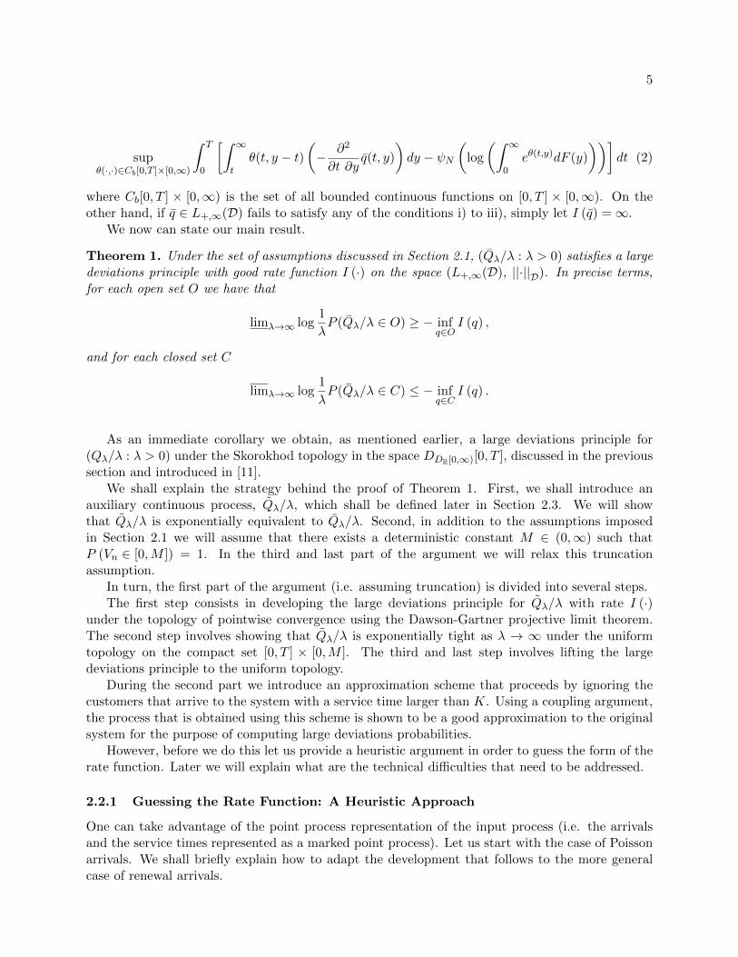
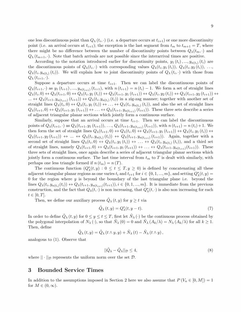
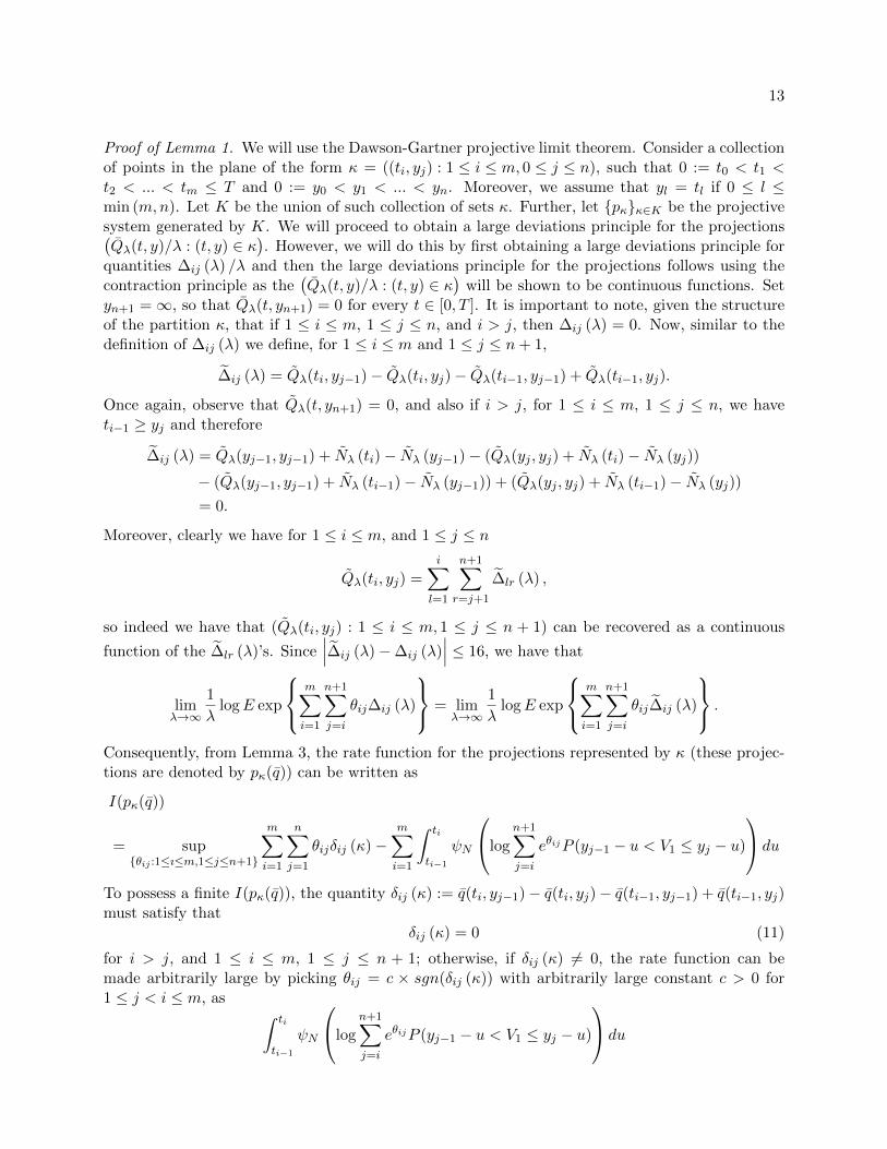
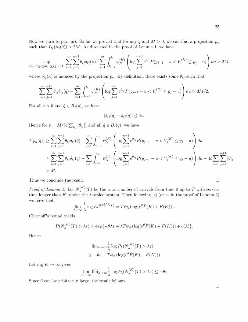
It is best to proceed our analysis by keeping in mind the pictorial representation that we shalldescribe. One can represent the arrival and status of each customer in a two-dimensional plane,with x-axis representing the arrival time and y-axis the service time at the time of arrival. Underthis representation, Qλ(t, y) is the number of points in the triangle formed by a vertical line and

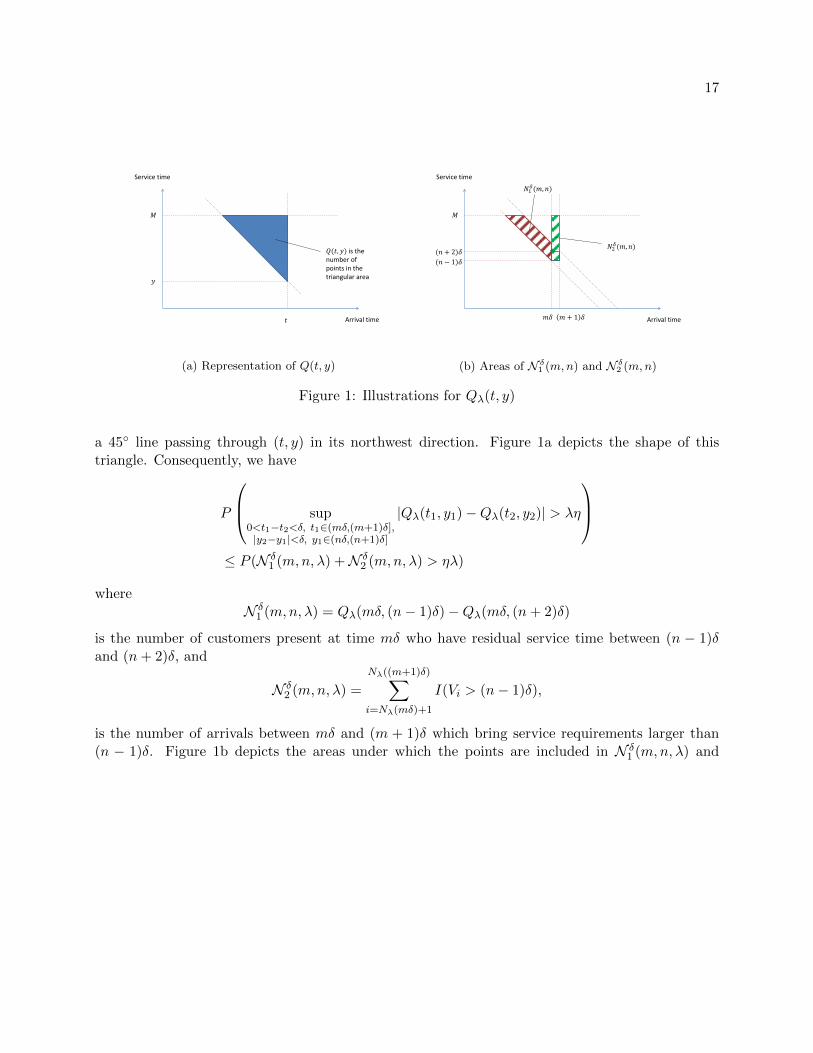
17

Arrival time

Service time

𝑀

𝑡

𝑄(𝑡, 𝑦) is the number of points in the triangular area

𝑦

(a) Representation of Q(t, y)

Arrival time

Service time

𝑀

𝑚𝛿

𝑁1𝛿(𝑚, 𝑛)

𝑚 + 1 𝛿

(𝑛 − 1)𝛿

(𝑛 + 2)𝛿 𝑁2𝛿(𝑚, 𝑛)

(b) Areas of N δ1 (m,n) and N δ

2 (m,n)

Figure 1: Illustrations for Qλ(t, y)

a 45◦ line passing through (t, y) in its northwest direction. Figure 1a depicts the shape of thistriangle. Consequently, we have

P

sup0<t1−t2<δ, t1∈(mδ,(m+1)δ],|y2−y1|<δ, y1∈(nδ,(n+1)δ]

|Qλ(t1, y1)−Qλ(t2, y2)| > λη

≤ P (N δ

1 (m,n, λ) +N δ2 (m,n, λ) > ηλ)

whereN δ

1 (m,n, λ) = Qλ(mδ, (n− 1)δ)−Qλ(mδ, (n+ 2)δ)

is the number of customers present at time mδ who have residual service time between (n − 1)δand (n+ 2)δ, and

N δ2 (m,n, λ) =

Nλ((m+1)δ)∑i=Nλ(mδ)+1

I(Vi > (n− 1)δ),

is the number of arrivals between mδ and (m + 1)δ which bring service requirements larger than(n − 1)δ. Figure 1b depicts the areas under which the points are included in N δ

1 (m,n, λ) and

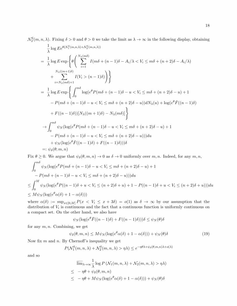
18

N δ2 (m,n, λ). Fixing δ > 0 and θ > 0 we take the limit as λ→∞ in the following display, obtaining

1

λlogEeθ(N

δ1 (m,n,λ)+N δ2 (m,n,λ))

=1

λlogE exp

{θ

(Nλ(mδ)∑i=1

I(mδ + (n− 1)δ −Ai/λ < Vi ≤ mδ + (n+ 2)δ −Ai/λ)

+

Nλ((m+1)δ)∑i=Nλ(mδ)+1

I(Vi > (n− 1)δ)

)}

=1

λlogE exp

{∫ mδ

0log(eθP (mδ + (n− 1)δ − u < Vi ≤ mδ + (n+ 2)δ − u) + 1

− P (mδ + (n− 1)δ − u < Vi ≤ mδ + (n+ 2)δ − u))dNλ(u) + log(eθF ((n− 1)δ)

+ F ((n− 1)δ))[Nλ((m+ 1)δ)−Nλ(mδ)]

}

→∫ mδ

0ψN (log(eθP (mδ + (n− 1)δ − u < Vi ≤ mδ + (n+ 2)δ − u) + 1

− P (mδ + (n− 1)δ − u < Vi ≤ mδ + (n+ 2)δ − u)))du

+ ψN (log(eθF ((n− 1)δ) + F ((n− 1)δ)))δ

=: ψδ(θ;m,n)

Fix θ ≥ 0. We argue that ψδ(θ,m, n)→ 0 as δ → 0 uniformly over m,n. Indeed, for any m,n,∫ mδ

0ψN (log(eθP (mδ + (n− 1)δ − u < Vi ≤ mδ + (n+ 2)δ − u) + 1

− P (mδ + (n− 1)δ − u < Vi ≤ mδ + (n+ 2)δ − u)))du

≤∫ M

0ψN (log(eθP ((n− 1)δ + u < Vi ≤ (n+ 2)δ + u) + 1− P ((n− 1)δ + u < Vi ≤ (n+ 2)δ + u)))du

≤ MψN (log(eθα(δ) + 1− α(δ)))

where α(δ) := supx∈[0,M ] P (x < Vi ≤ x + 3δ) = o(1) as δ → ∞ by our assumption that thedistribution of Vi is continuous and the fact that a continuous function is uniformly continuous ona compact set. On the other hand, we also have

ψN (log(eθF ((n− 1)δ) + F ((n− 1)δ)))δ ≤ ψN (θ)δ

for any m,n. Combining, we get

ψδ(θ,m, n) ≤MψN (log(eθα(δ) + 1− α(δ))) + ψN (θ)δ (19)

Now fix m and n. By Chernoff’s inequality we get

P (N δ1 (m,n, λ) +N δ

2 (m,n, λ) > ηλ) ≤ e−ηθλ+ψδ(θ,m,n)λ+o(λ)

and so

limλ→∞1

λlogP (N1(m,n, λ) +N2(m,n, λ) > ηλ)

≤ − ηθ + ψδ(θ,m, n)

≤ − ηθ +MψN (log(eθα(δ) + 1− α(δ))) + ψN (θ)δ

19

by (19). Hence

limλ→∞1

λlogP

(w

(Qλλ, δ

)> η

)

≤ limλ→∞1

λlog

bT/δc∑m=0

bM/δc∑n=0

P (N δ1 (m,n, λ) +N δ

2 (m,n, λ) > ηλ)

≤ − ηθ +MψN (log(eθα(δ) + 1− α(δ))) + ψN (θ)δ

which gives

limδ→0

lim supλ→∞

1

λlogP

(w

(Qλλ, δ

)> η

)≤ −ηθ

Since θ can be arbitrarily large, we conclude (17). Finally, condition (18) follows from the analysisof N δ

2 (m, 1, λ)/λ.

4 Unbounded Service Times

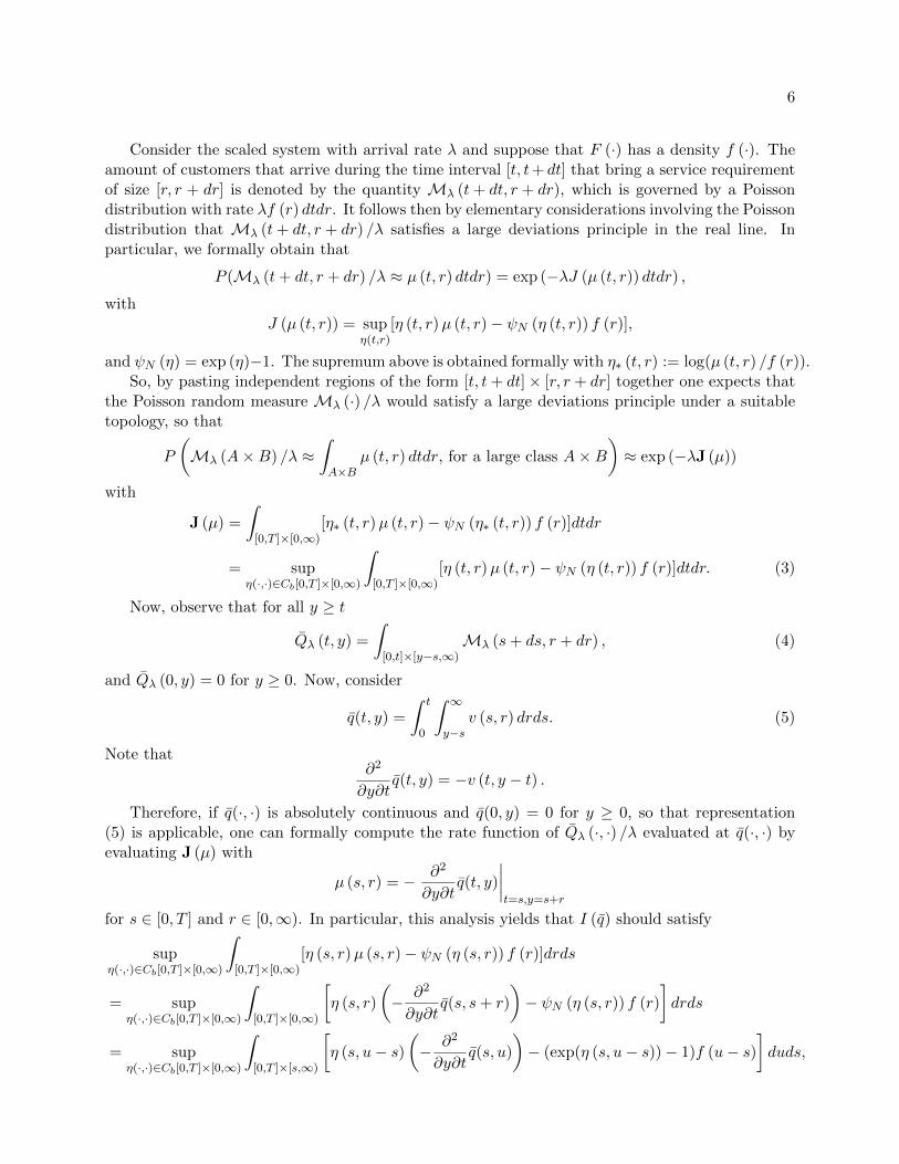
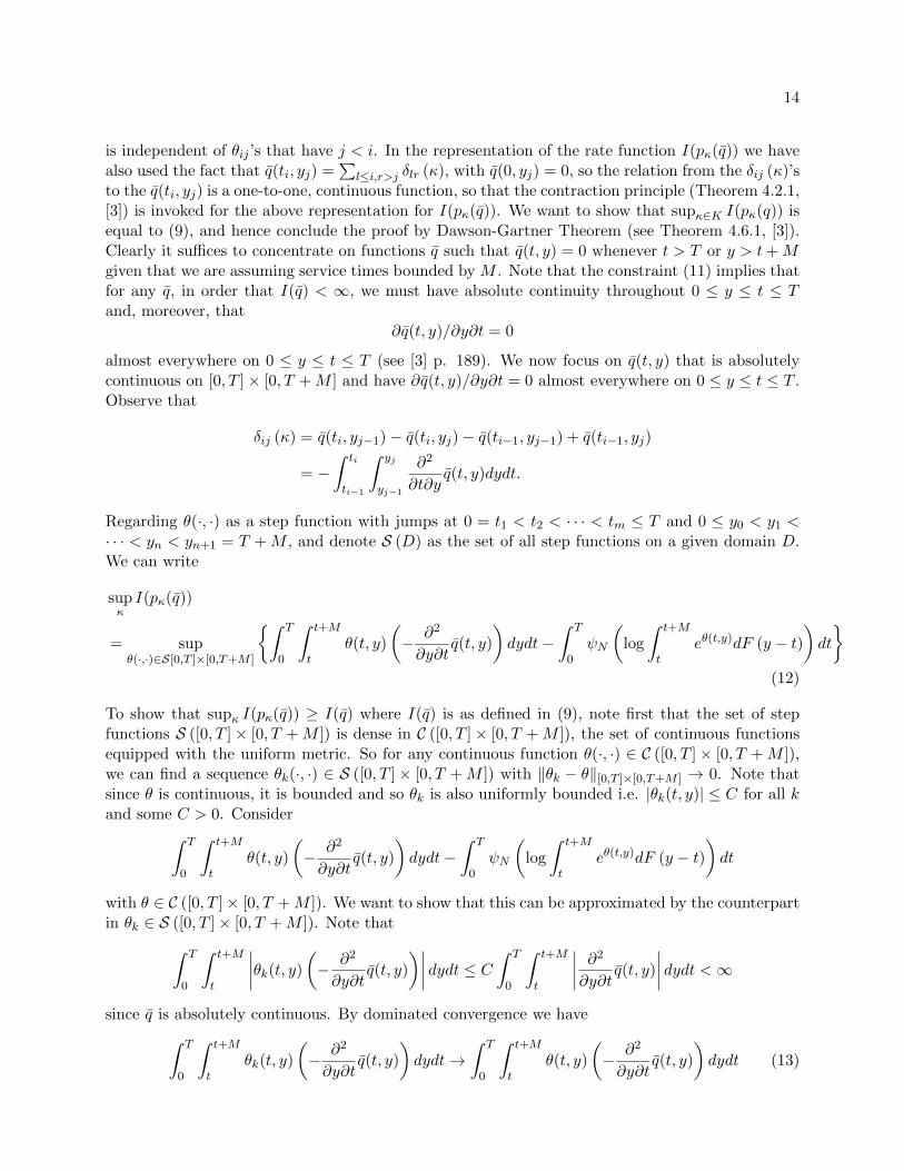
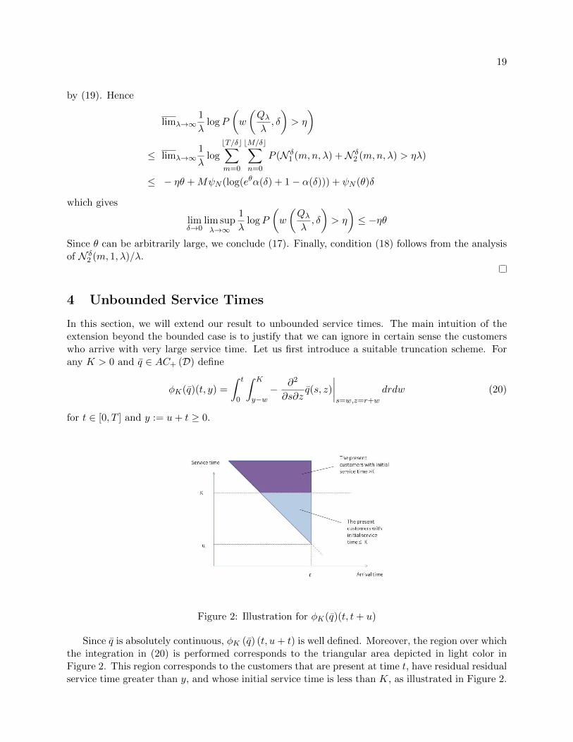
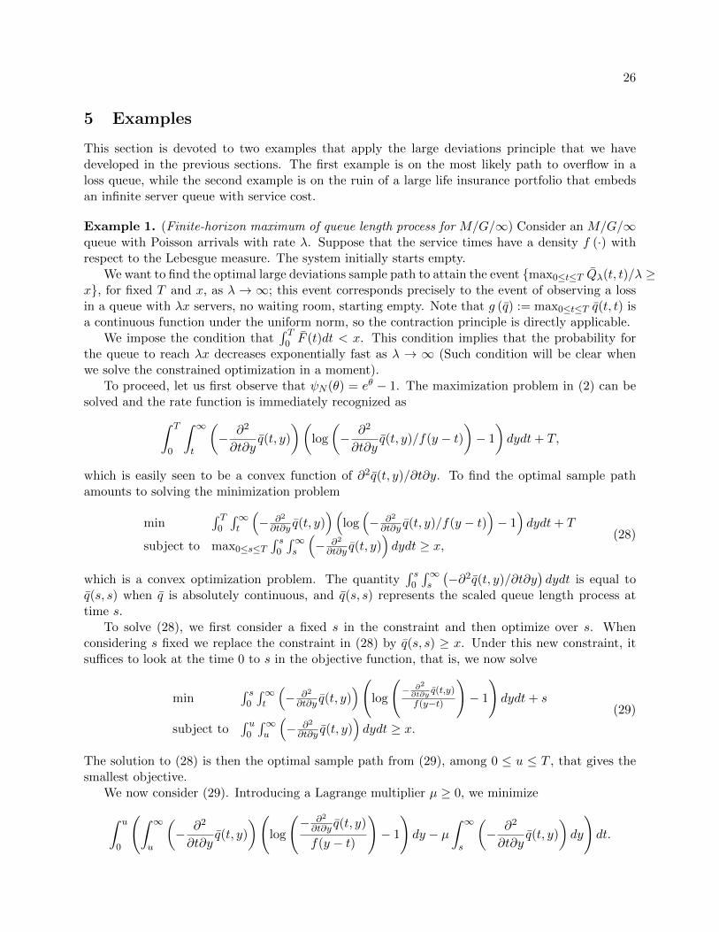
In this section, we will extend our result to unbounded service times. The main intuition of theextension beyond the bounded case is to justify that we can ignore in certain sense the customerswho arrive with very large service time. Let us first introduce a suitable truncation scheme. Forany K > 0 and q ∈ AC+ (D) define

φK(q)(t, y) =

∫ t

0

∫ K

y−w− ∂2

∂s∂zq(s, z)

∣∣∣∣s=w,z=r+w

drdw (20)

for t ∈ [0, T ] and y := u+ t ≥ 0.

Figure 2: Illustration for φK(q)(t, t+ u)

Since q is absolutely continuous, φK (q) (t, u+ t) is well defined. Moreover, the region over whichthe integration in (20) is performed corresponds to the triangular area depicted in light color inFigure 2. This region corresponds to the customers that are present at time t, have residual residualservice time greater than y, and whose initial service time is less than K, as illustrated in Figure 2.

20

Moreover, for a sample path Qλ, define Qλ,K as the two-parameter process derived from Qλ byignoring the arrivals with service time greater than K (one way to imagine is that they leave thesystem immediately upon arrival). Therefore, Qλ,K is a two-parameter queue length process corre-

sponding to an infinite server system with i.i.d. interarrival times following the law U =∑G

i=1 Ui/λ,where G is a geometric r.v. independent of the Ui’s such that P (G = n) = F (K)n−1F (K), n ≥ 1.It is easy to check that the arrival process corresponding to Qλ,K , i.e. by ignoring the arrivals withinitial service time larger than K, satisfies the conditions in Section 2.1. The service time then has

the distribution function FK(x) = F (x)/F (K) for x ∈ [0,K]. We denote (V(K)n , n = 1, . . .) as the

sequence of service times in this modified system.Now recall the continuous version of Qλ, denoted by Qλ constructed in Section 2.3. Moreover,

define Qλ,K to be the continuous approximation to Qλ,K constructed in exactly the same fashion.In addition, for q ∈ AC+ (DK) define IK (q) as

supθ(t,·)∈C[0,T ]×[0,T+K]

∫ T

0

[∫ t+K

tθ(t, y − t)

(− ∂2

∂t ∂yq(t, y)

)dy − ψ(K)

N

(log

(1

F (K)

∫ K

0eθ(t,y)dF (y)

))]dt,

(21)

and set IK (q) = ∞ otherwise, where ψ(K)N is the infinitesimal moment generating function corre-

sponding to the truncated arrival process.Theorem 2 yields that Qλ,K/λ, satisfies a full large deviations principle with good rate function

IK(·). For q ∈ AC+ (D) we shall also evaluate IK (q) according to the expression (21).Since the geometric r.v. G is independent of the Ui’s, we can compute the associated logarithmic

moment generating function of the modified interarrival times

κ(K)(θ) := κ(θ) + log

(F (K)

1− F (K)eκ(θ)

),

and from which we solve that the associated infinitesimal logarithmic moment generating functionof the arrival process is

ψ(K)N (θ) := ψN (log(F (K)eθ + F (K))).

Plugging in the above expressions into (21), we have the following expression of IK(q)

supθ(·,·)∈C[0,T ]×[0,T+K]

∫ T

0

[∫ T+K

tθ(t, y − t)

(− ∂2

∂t ∂yq(t, y)

)dy − ψN

(log

(F (K) +

∫ K

0eθ(t,y)dF (y)

))]dt.

(22)At this point our strategy involves two steps. First, we want to show that Qλ,K/λ and Qλ,K/λ

are exponentially good approximations as K ↗∞ to both Qλ/λ and Qλ/λ respectively. The secondstep consists in using this fact, together with the properties of IK(q) as K ↗∞ and also propertiesof I (q) to conclude the identification of the rate function of Qλ/λ.

So, to execute the first step we first define

N(K)λ (t) =

Nλ(t)∑j=1

I (Vj > K) ,

that is, N(K)λ (t) is the number of arrivals with service time larger than K in the λ-scaled system.

Then we obtain the following result, which is proved at the end of this section.

21

Lemma 4. For any ε > 0,

limK→∞

limλ→∞1

λlogP (N

(K)λ (T ) > λε) = −∞. (23)

Consequently, Qλ,K/λ and Qλ,K/λ are exponentially good approximations as K ↗∞ to both Qλ/λand Qλ/λ respectively.

Using the previous lemma we obtain the following result. The proof is straightforward, butfollowing our convention we shall give it at the end of the section.

Lemma 5. The family (Qλ/λ : λ > 0) satisfies a weak large deviations principle on C+ (D) withrate function

I∗ (q) := supδ>0

limK→∞ inf{z:||z−q||D≤δ}

IK (z) .

We now extend the weak large deviations principle into a full large deviations principle with agood rate function using exponential tightness.

Lemma 6. The family (Qλ/λ : λ > 0) is exponentially tight on C+ (D) and therefore it satisfies afull large deviations principle with good rate function I∗ (·) .

We proceed to show the identification I∗ (q) = I (q). We now collect useful properties that wewill need to show this identification.

Lemma 7.

i) For any q such that I(q) <∞, we have I(φK(q)) = IK(φK(q)) = IK(q)↗ I(q) as K →∞;the notation IK(q)↗ I(q) implies that (IK(q) : K > 0) is non decreasing in K and convergent toI(q).

ii) For any q such that I(q) =∞, and each M > 0, there exists a projection pκ (following thenotation introduced in the proof of Lemma 1) such that, for large enough K,

IK(pκ(q)) > M.

iii) Finally, with κ from ii) there exists ε > 0 such that if q ∈ C+ (D) and ||q − q||D < ε then

IK(pκ(q)) > M.

We now are ready to prove the following important result of this section.

Theorem 3. Qλ/λ satisfies a large deviations principle with good rate function defined in (2) underthe uniform topology on [0, T ]× [0,∞).

Proof of Theorem 3. Given Lemma 6 all we need to show is that I∗ (q) = I (q). Suppose that q issuch that I (q) =∞. Then, parts ii) and iii) in Lemma 7 imply in particular that for every M , thereexists K, a projection κ, and ε > 0 such that IK (pκ (q)) > M for any ||q − q||D < ε. Consequently,we conclude, by using the monotonicity of IK (q) as a function of K and taking subsequences, that

I∗ (q) = supδ>0

limK→∞ inf{z:||z−q||D≤δ}

IK (z) = supδ>0

supK>0

inf{z:||z−q||D≤δ}

IK (z) =∞.

22

If I (q) <∞, then note that

I∗ (q) = supδ>0

supK>0

inf{z:||z−q||D≤δ}

IK (z) = supK>0

supδ>0

inf{z:||z−q||D≤δ}

IK (z) .

Further, observe that

supδ>0

inf{z:||z−q||D≤δ}

IK (z) = supδ>0

inf{φK(z):||φK(z)−φK(q)||D≤δ}

IK (φK (z)) ,

Since IK (·) is a rate function (in particular IK (·) is lower semicontinuous) we have that

supδ>0

inf{φK(z):||φK(z)−φK(q)||DK≤δ}

IK (φK (z)) = IK (φK (q))

and then by part i) of Lemma 7 we conclude that supK>0 IK (φK (q)) = I (q), thus concluding thatI∗ (q) = I (q) as claimed.

We finish this section with the proof of Theorem 1.

Proof of Theorem 1. All we need to show is that Qλ/λ and Qλ/λ are exponentially equivalent. Thisfollows exactly as in the proof of Corollary 1 since ‖Qλ− Qλ‖D ≤ 4. The measurability issue againis dealt with using separability. The result then follows by applying Theorem 4.2.13 in [3].

4.1 Proofs of Technical Results

We now provide the proof of the pending technical results.

Proof of Lemma 5. This result is a direct application of part a) in Theorem 4.2.16 in [3].

Proof of Lemma 6. This is similar to the case with bounded service time, but the conditions fortightness are slightly different given that our domain D is not compact. We must show that for anyη, γ > 0, we can choose small enough ρ > 0, such that for δ < ρ,

1

λlogP (w(Qλ/λ, δ) > η) < −γ

when λ is large; this part is indeed basically the same as the case DM . In addition, however, wealso must show that for all η > 0 and every a > 0 there exists K > 0 such that

P

(supt∈[0,T ]

supy≥K

Qλ (t, y) /λ > η

)≤ exp (−λa) . (24)

Note that

P (w(Qλ/λ, δ) > η)

≤P(w(Qλ/λ, δ) > η, ‖Qλ/λ− Qλ,K/λ‖ ≤

η

2

)+ P

(‖Qλ/λ− Qλ,K/λ‖ >

η

2λ)

≤P(w(Qλ,K/λ, δ) >

η

2

)+ P

(N

(K)λ (T ) > λη/2

), (25)

23

and

P

(supt∈[0,T ]

supy≥K

Qλ (t, y) /λ > η

)≤ P

(N

(K)λ (T ) > λη

).

By Lemma 4, for every γ > 0 can choose K large enough such that

1

λlogP

(N

(K)λ (T ) > λη/2

)< −2γ.

for all λ large enough. So, condition (24) is enforced and the second term in the sum in (25) is alsoappropriately controlled. Now, by a similar argument as in Lemma 2 in the previous section, for achosen K, we have, for all small enough δ,

1

λlogP

(w(Qλ,K/λ, δ) >

η

2

)< −2γ.

for large enough λ. In sum, we get

1

λlogP (w(Qλ/λ, δ) > η) < −γ

for large enough λ. Therefore, exponential tightness follows. It follows immediately that a weaklarge deviations principle and exponential tightness implies a full large deviations principle. Thegoodness of the rate function then is a consequence of exponential tightness together with the weaklarge deviations principle; see Lemma 1.2.18, p. 8, part b) of [3].

Proof of Lemma 7. We start with part i), assuming that I(q) <∞. Since

∂2

∂t∂yφK(q)(t, y) =

∂2

∂y∂tφK(q)(t, y) =

∂2

∂t∂yq(t, y)1{y≤K+t},

we have immediately that I(φK(q)) = IK(φK(q)) = IK(q). It is obvious that IK(q) is non-decreasingin K and that IK (q) ≤ I(q). On the other hand, there exists θn ∈ Cb[0, T ] × [0,∞) (the space ofbounded and continuous functions on [0, T ]× [0,∞)) such that

In(q) :=

∫ T

0

[∫ ∞t

θn(t, y − t)(− ∂2

∂t ∂yq(t, y)

)dy − ψN

(log

(∫ ∞0

eθn(t,y)dF (y)

))]dt

converges to I(q) as n → ∞. Since I(q) < ∞, it follows easily that ∂2q(·)/∂t∂y is integrable overD. Therefore, given that θn(·) is bounded,∫ T

0

∫ ∞K

θn(t, y − t)(− ∂2

∂t ∂yq(t, y)

)dydt→ 0

as K → ∞. Besides, for given n, as ψN is uniformly continuous on the bounded set [−Mn,Mn]where Mn = sup |θn(t, y)| <∞, we have that

ψN

(log

(F (K) +

∫ K

0eθn(t,y)dF (y)

))converges to

ψN

(log

(∫ ∞0

eθn(t,y)dF (y)

))

24

uniformly on t ∈ [0, T ]. In sum, limK→∞InK(q) = In(q) as K →∞. Therefore, there exists Kn such

that InKn(q) ≥ In(q)− 1/n. Recall that InKn(q) ≤ IKn(q) and consequently we obtain

In(q)− 1

n≤ IKn(q) ≤ I(q).

Since IK(q) increases in K, we have IK(q)↗ I(q) as claimed.For part ii), when I(q) = ∞, there are two cases: a) q is not absolutely continuous, and b) q isabsolutely continuous. Case b) in turn is divided into two subcases: b.1) ∂2q(t, y)/∂t ∂y is notintegrable over D, and b.2) ∂2q(t, y)/∂t ∂y is integrable over D. We shall proceed to analyze allthese cases now. For Case a). We can construct a projection pκ with IK(pκ(q)) > M as we did inthe proof of Lemma 1. For Case b), we have that q is absolutely continuous, but

supθ(·,·)∈Cb[0,T ]×[0,∞)

∫ T

0

[∫ ∞0

θ(t, y)

(− ∂2

∂t ∂yq(t, y + t)

)dy − ψN

(log

(∫ ∞0

eθ(t,y)dF (y)

))]dt =∞,

so we proceed to study case b.1): Assume that ∂2q(t, y)/∂t ∂y is not integrable on D. We shallassume that ∫ T

0

∫ ∞t

(− ∂2

∂t ∂yq(t, y)

)+

dydt =∞ (26)

(if this integral is finite, then integral of the negative part must diverge and the analysis that followsnext is identical). As in the proof of Lemma 1, given a projection κ induced by 0 ≤ t1 < t2 < ... <tm ≤ T and 0 ≤ y0 < y1 < ... < yn+1, define

δij (κ) := q(ti, yj−1)− q(ti, yj)− q(ti−1, yj−1) + q(ti−1, yj)

= −∫ ti

ti−1

∫ yj

yj−1

∂2

∂y∂tq(t, y)dydt, (27)

as long as yj−1 ≥ ti−1 (otherwise, if yj−1 < ti−1, δij (κ) = 0). Then, from (26) and (27), it followseasily that for any M , there exists a partition κ such that∑

i,j

δij (κ) > M + TψN (1).

Therefore, for large enough K,

IK(pκ (q)) ≥∑i,j

δij (κ)− TψN (1) > M.

Now, for case b.2) suppose that ∂2q(t, y)/∂t ∂y is integrable on D. We can find θ(t, y) such that

3M <

∫ T

0

∫ ∞t

θ(t, y − t)(− ∂2

∂t ∂yq(t, y)

)dy − ψN

(log

(∫ ∞0

eθ(t,y)dF (y)

))dt <∞.

Following the same line of reasoning as in the proof of part i) we can conclude that there existsK > 0 such that IK(q) > 2M . According to Dawson-Gartner Theorem, IK(q) = sup IK(pκ(q))where the supremum is taken over all projections restricted to {t ∈ [0, T ], 0 ≤ y ≤ t + K}. As aresult, there exists some projection pκ such that IK(pκ(q)) > M and hence we are done.

25

Now we turn to part iii). So far we proved that for any q and M > 0, we can find a projection pκsuch that IK(pκ(q)) > 2M . As discussed in the proof of Lemma 1, we have

sup{θij :1≤i≤m,1≤j≤n+1}

m∑i=1

n+1∑j=1

θijδij(κ)−m∑i=1

∫ ti

ti−1

ψ(K)N

log

n+1∑j=1

eθijP (yj−1 − u < V(K)

1 ≤ yj − u)

du > 2M.

where δij(κ) is induced by the projection pκ. By definition, there exists some θij such that

m∑i=1

n+1∑j=1

θijδij(q)−m∑i=1

∫ ti

ti−1

ψ(K)N

log

n+1∑j=1

eθijP (yj−1 − u < V(K)

1 ≤ yj − u)

du > 3M/2.

For all ε > 0 and q ∈ Bε(p), we have

|δij(q)− δij(q)| ≤ 4ε.

Hence for ε = M/(8∑

i,j |θij |) and all q ∈ Bε(q), we have

I(pκ(q)) ≥m∑i=1

n+1∑j=1

θijδij(q)−m∑i=1

∫ ti

ti−1

ψ(K)N

log

n+1∑j=1

eθijP (yj−1 − u < V(K)

1 ≤ yj − u)

du

≥m∑i=1

n+1∑j=1

θijδij(q)−m∑i=1

∫ ti

ti−1

ψ(K)N

log

n+1∑j=1

eθijP (yj−1 − u < V(K)

1 ≤ yj − u)

du− 4ε

m∑i=1

n+1∑j=1

|θij |

> M.

Thus we conclude the result.

Proof of Lemma 4. Let N(K)λ (T ) be the total number of arrivals from time 0 up to T with service

time longer than K, under the λ-scaled system. Then following [4] (or as in the proof of Lemma 2)we have that

limλ→∞

1

λlogEeθN

(K)λ (T ) = TψN (log(eθF (K) + F (K))).

Chernoff’s bound yields

P (N(K)λ (T ) > λε) ≤ exp{−θλε+ λTψN (log(eθF (K) + F (K))) + o(λ)}.

Hence

limλ→∞1

λlogPλ(N

(K)λ (T ) > λε)

≤− θε+ TψN (log(eθF (K) + F (K)))

Letting K →∞ gives

limK→∞

limλ→∞1

λlogPλ(N

(K)λ (T ) > λε) ≤ −θε

Since θ can be arbitrarily large, the result follows.

26

5 Examples

This section is devoted to two examples that apply the large deviations principle that we havedeveloped in the previous sections. The first example is on the most likely path to overflow in aloss queue, while the second example is on the ruin of a large life insurance portfolio that embedsan infinite server queue with service cost.

Example 1. (Finite-horizon maximum of queue length process for M/G/∞) Consider an M/G/∞queue with Poisson arrivals with rate λ. Suppose that the service times have a density f (·) withrespect to the Lebesgue measure. The system initially starts empty.

We want to find the optimal large deviations sample path to attain the event {max0≤t≤T Qλ(t, t)/λ ≥x}, for fixed T and x, as λ → ∞; this event corresponds precisely to the event of observing a lossin a queue with λx servers, no waiting room, starting empty. Note that g (q) := max0≤t≤T q(t, t) isa continuous function under the uniform norm, so the contraction principle is directly applicable.

We impose the condition that∫ T

0 F (t)dt < x. This condition implies that the probability forthe queue to reach λx decreases exponentially fast as λ → ∞ (Such condition will be clear whenwe solve the constrained optimization in a moment).

To proceed, let us first observe that ψN (θ) = eθ − 1. The maximization problem in (2) can besolved and the rate function is immediately recognized as∫ T

0

∫ ∞t

(− ∂2

∂t∂yq(t, y)

)(log

(− ∂2

∂t∂yq(t, y)/f(y − t)

)− 1

)dydt+ T,

which is easily seen to be a convex function of ∂2q(t, y)/∂t∂y. To find the optimal sample pathamounts to solving the minimization problem

min∫ T

0

∫∞t

(− ∂2

∂t∂y q(t, y))(

log(− ∂2

∂t∂y q(t, y)/f(y − t))− 1)dydt+ T

subject to max0≤s≤T∫ s

0

∫∞s

(− ∂2

∂t∂y q(t, y))dydt ≥ x,

(28)

which is a convex optimization problem. The quantity∫ s

0

∫∞s

(−∂2q(t, y)/∂t∂y

)dydt is equal to

q(s, s) when q is absolutely continuous, and q(s, s) represents the scaled queue length process attime s.

To solve (28), we first consider a fixed s in the constraint and then optimize over s. Whenconsidering s fixed we replace the constraint in (28) by q(s, s) ≥ x. Under this new constraint, itsuffices to look at the time 0 to s in the objective function, that is, we now solve

min∫ s

0

∫∞t

(− ∂2

∂t∂y q(t, y))(

log

(− ∂2

∂t∂yq(t,y)

f(y−t)

)− 1

)dydt+ s

subject to∫ u

0

∫∞u

(− ∂2

∂t∂y q(t, y))dydt ≥ x.

(29)

The solution to (28) is then the optimal sample path from (29), among 0 ≤ u ≤ T , that gives thesmallest objective.

We now consider (29). Introducing a Lagrange multiplier µ ≥ 0, we minimize

∫ u

0

(∫ ∞u

(− ∂2

∂t∂yq(t, y)

)(log

(− ∂2

∂t∂y q(t, y)

f(y − t)

)− 1

)dy − µ

∫ ∞s

(− ∂2

∂t∂yq(t, y)

)dy

)dt.

27

By a formal application of Euler-Lagrange equations, we differentiate the integrand with respect to−∂2q(t, y)/∂t∂y to get log

(−∂2q(t,y)/∂t∂y

f(t−y)

)= 0 for t ≤ y ≤ u

log(−∂2q(t,y)/∂t∂y

f(t−y)

)− µ = 0 for y > u

which gives

− ∂2

∂t∂yq(t, y) =

{f(y − t) for t ≤ y ≤ uµf(y − t) for y > u

for some µ ≥ 1 (we replace eµ by another dummy µ for convenience). Complementary slacknessthen implies ∫ u

0

∫ ∞u

(−∂2q(t, y)/∂t∂y)dydt =

∫ u

0

∫ ∞u

µf(y − t)dydt = x,

which in turn gives

µ =x∫ u

0 F (t)dt

(note that we have assumed∫ u

0 F (t)dt < x and so the condition µ > 1 is satisfied). As a result

− ∂2

∂t∂yq(t, y) =

{f(y − t) for t ≤ y ≤ uxf(y−t)∫ u0 F (t)dt

for y > u.

The optimal sample path q(t, y) leading to the constraint q(u, u) ≥ x is given by

q(t, y) =

∫ t

0

∫ ∞y

(− ∂2

∂t∂yq(s, w)

)dwds

=

∫ t

0

(∫ u

y∧uf(w − s)dw +

∫ ∞u∨y

xf(w − s)∫ u0 F (r)dr

dw

)ds

Transforming into q(t, y) = q(t, y + t) and some simple calculus gives the optimal sample path

q(t, y) =

∫ y+t

yF (s)ds−

∫ u

u−tF (s)ds+

x∫ uu−t F (s)ds∫ u0 F (r)dr

, for y + t ≤ u,

and

q(t, y) =x∫ y+ty F (s)ds∫ u0 F (r)dr

, for y + t > u.

In connection to our discussion about the direct rate function representation in terms of Qλ/λ(see equation (6), in Section 2.2.1), one can check that ∂q(t, y)/∂y is not continuous on the liney = t and therefore ∂2q(t, y)/∂y2 does not exists though I(q) is finite.

Note also that the objective is∫ u

0

(−∫ u

tf(y − t)dy +

∫ ∞u

xf(y − t)∫ u0 F (t)dt

(log

(x∫ u

0 F (t)dt

)− 1

)dy

)dt+ T

=

∫ u

0F (t)dt+

(log

(x∫ s

0 F (t)dt

)− 1

)x. (30)

28

This is the rate function corresponding to the probability P (Qλ(u, u) ≥ λx) = P (Qλ(u, 0) ≥ λx),where Qλ(u, 0) is the queue length at time u. This rate of decay is consistent with direct calculationusing the fact that Qλ(u, 0) is a Poisson random variable with rate λ

∫ u0 F (t)dt, which gives

P (Q(s) > λx) =∑n≥λx

e−λ∫ u0 F (t)dt

(λ

∫ u

0F (t)dt

)n/n!.

For a consistency check, our result here can in fact recover the large deviations for the arrival

process itself. If one changes the constraint in (29) to q(u, 0) =∫ u

0

∫∞0

(− ∂2

∂t∂y q(t, y))dydt ≥ x, the

optimal value of (29) then becomes x[log(x/s)− 1] + s, which coincides with the exponential decayrate of P (Poisson(λs) > λx) as λ→∞.

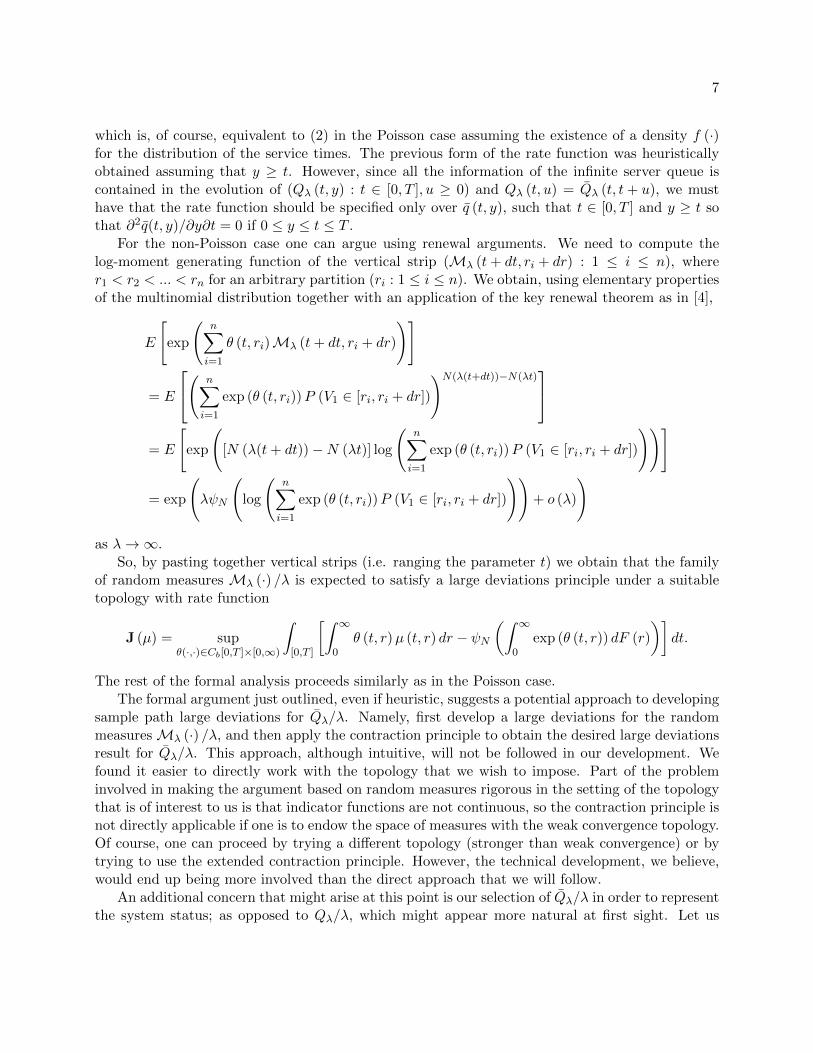
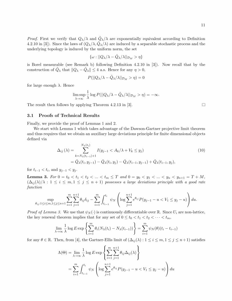
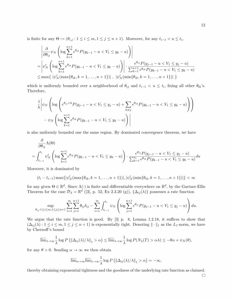
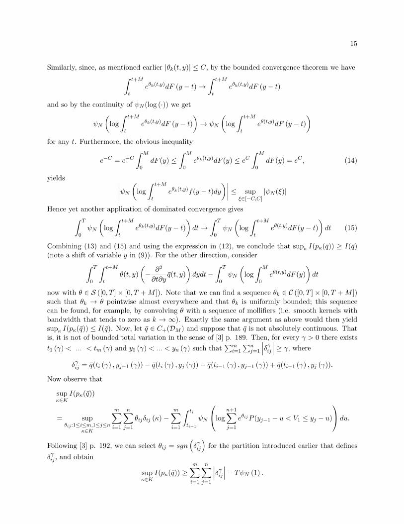
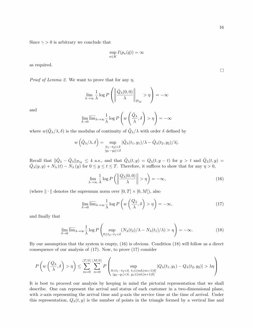
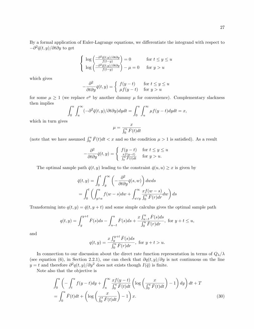
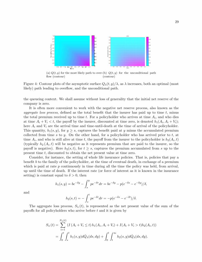
Figures 3 and 4 illustrate both the law of large numbers (i.e. the typical path) and the mostlikely path to the overflow event max0≤u≤T Qλ(u, u)/λ ≥ x for T = 1, x = 2. The underlyingservice time distribution is uniform in the interval [0, 1]. We can see that the optimal path ofQ(t, y) increases gradually over time to overflow at time 1.

(a) Q(t, y) for the most likely path to overflow (sur-face)

(b) Q(t, y) for the unconditional path (surface)

Figure 3: Surface plots of the asymptotic surface Qλ(t, y)/λ, as λ increases, both an optimal (mostlikely) path leading to overflow, and the unconditional path.

It is easy to see that since we assume∫ T

0 F (u)du < x, the rate function (30) is non-decreasingin s, and as a result an optimal time horizon is T . If the service time has bounded support [0,M ]with M < T , then the selection of any time s ∈ [M,T ] will give an optimal sample path.

Example 2. (Insurance risk process) The net reserve of a life insurance company consists ofthe premium collected from policyholders, deducted by the benefit paid to policyholders in theevent of deaths; often all these payments are discounted at zero in order to recognize the valueof money in time. When policyholders arrive at the insurance company over time (an arrival isinterpreted as the moment when a contract is signed), one can model the net assets of the insureras a function of the underlying arrivals and death events of policyholders. Specifically, we shallassume that policyholders arrive according to a Poisson process with rate λ, and that the time-until-death upon arrival of the policyholders are independent and identically distributed. Moreover,we assume that the time-until-death upon arrival has density f(·), distribution function F (·), andtail distribution F (·). The time-until-death in this setting can be thought as the service time in

29

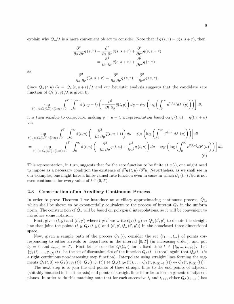
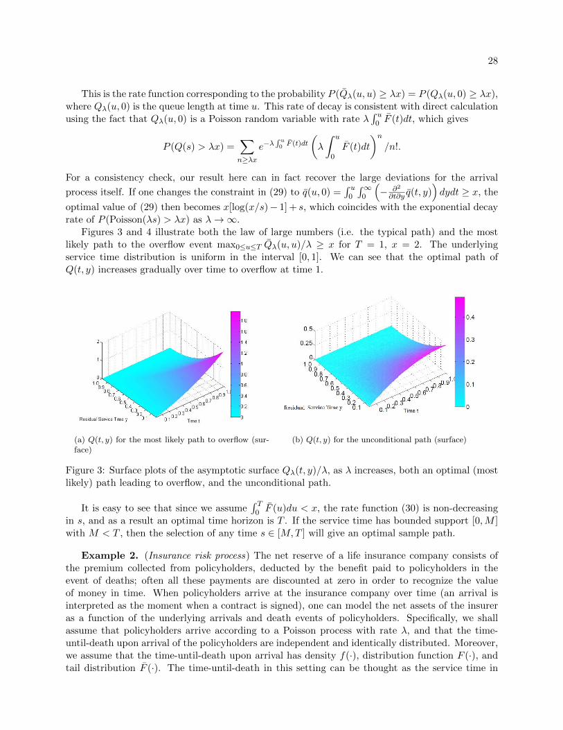
(a) Q(t, y) for the most likely path to over-flow (contour)

0.1 0.2 0.3 0.4 0.5 0.6 0.7 0.8 0.9 1.0

0.1

0.2

0.3

0.4

0.5

0.6

0.7

0.8

0.9

1.0 q(t,y)

Time t

Res

idua

l Ser

vice

Tim

e y

0

0.05

0.1

0.15

0.2

0.25

0.3

0.35

0.4

0.45

(b) Q(t, y) for the unconditional path(contour)

Figure 4: Contour plots of the asymptotic surface Qλ(t, y)/λ, as λ increases, both an optimal (mostlikely) path leading to overflow, and the unconditional path.

the queueing context. We shall assume without loss of generality that the initial net reserve of thecompany is zero.

It is often more convenient to work with the negative net reserve process, also known as theaggregate loss process, defined as the total benefit that the insurer has paid up to time t, minusthe total premium received up to time t. For a policyholder who arrives at time Ai, and who diesat time Ai + Vi < t, the payoff by the insurer, discounted at time zero, is denoted h1(Ai, Ai + Vi);here Ai and Vi are the arrival time and time-until-death at the time of arrival of the policyholder.This quantity, h1(s, y), for y ≥ s, captures the benefit paid at y minus the accumulated premiumcollected from time s to y. On the other hand, for a policyholder who has arrived prior to t, attime Ai, and who is still alive at time t, the payoff from the insurer to the policyholder is h2(Ai, t)(typically h2 (Ai, t) will be negative as it represents premium that are paid to the insurer, so thepayoff is negative). Here h2(s, t), for t ≥ s, captures the premium accumulated from s up to thepresent time t, discounted to obtain the net present value at time zero.

Consider, for instance, the setting of whole life insurance policies. That is, policies that pay abenefit b to the family of the policyholder, at the time of eventual death, in exchange of a premiumwhich is paid at rate p continuously in time during all the time the policy was held, from arrival,up until the time of death. If the interest rate (or force of interest as it is known in the insurancesetting) is constant equal to δ > 0, then

h1(s, y) = be−δy −∫ y

spe−δrdr = be−δy − p(e−δs − e−δy)/δ,

and

h2(s, t) = −∫ t

spe−δrdr = −p(e−δs − e−δt)/δ.

The aggregate loss process, Sλ (t), is represented as the net present value of the sum of thepayoffs for all policyholders who arrive before t and it is given by

Sλ (t) =

Nλ(t)∑i=1

(I (Ai + Vi ≤ t)h1(Ai, Ai + Vi) + I(Ai + Vi > t)h2(Ai, t))

=

∫ t

0

∫ t

sh1(s, y)dQλ(ds, dy) +

∫ t

0

∫ ∞t

h2(s, y)dQλ(ds, dy).

30

We claim that Sλ (·) is a continuous function of Qλ (·) under the uniform topology on D. In orderto see this, define Dλ (t) to be the number of departures by time t, that is,

Dλ (t) = Nλ (t)− Qλ (t, t) = Qλ (t, 0)− Qλ (t, t) . (31)

Note that Dλ (·) and Nλ (·) are clearly continuous functions of Qλ (·). Moreover, we have that

Nλ(t)∑i=1

I (Ai + Vi ≤ t)h1(Ai, Ai + Vi) =

∫ t

0

∫ t

0h1 (s, u)Dλ (du)Nλ (ds) ,

and therefore

Sλ (t) =

∫ t

0

∫ t

0h1 (s, u)Dλ (du)Nλ (ds) +

∫ t

0

∫ ∞t

h2(s, y)Qλ(ds, dy).

Now, integration by parts shows that∫ t

0

∫ t

0h1 (s, u)Dλ (du)Nλ (ds)

=

∫ t

0

∫ t

0

∂2

∂u∂sh1 (s, u)Dλ (u)Nλ (s) dsdu−Nλ (t)

∫ t

0Dλ (u)

∂

∂uh1 (t, u) du

−Dλ (t)

∫ t

0

∂

∂sh1 (s, t)Nλ (s) ds+Dλ (t)Nλ (t)h1 (t, t) . (32)

A similar development yields∫ t

0

∫ ∞t

h2(s, y)Qλ(ds, dy) =

∫ ∞t

∫ t

0Qλ(s, y)

∂2h2 (s, y)

∂s∂ydsdy −

∫ ∞t

Qλ(t, y)∂h2 (t, y)

∂ydy

+

∫ t

0

∂h2(s, t)

∂sQλ(s, t)ds− Qλ(t, t)h2 (t, t) . (33)

It is now not difficult to see from (32) and (33) that indeed Sλ (·) is a continuous function of Qλ (·)in the uniform topology on [0, T ]× [0,∞).

Consider the finite-horizon ruin probability that the negative net asset of the insurer rises abovethe level λx by time T . That is, the event {maxt∈[0,T ] Sλ (t) /λ ≥ x}. We wish to solve for the mostlikely path that leads to this event and therefore, applying our theory, we must solve the followingconvex calculus of variations problem.

min∫ T

0

∫∞t

(− ∂2

∂t∂y q(t, y))(

log

(− ∂2

∂t∂yq(t,y)

f(y−t)

)− 1

)dydt+ T

subject to max0≤u≤T∫ u

0

(∫ ut h1(t, y)

(− ∂2

∂t∂y q(t, y))dy +

∫∞u h2(t, u)

(− ∂2

∂t∂y q(t, y))dy)dt ≥ x

Following the recipe of Example 1, we first consider

min∫ u

0

∫∞t

(− ∂2

∂t∂y q(t, y))(

log

(− ∂2

∂t∂yq(t,y)

f(y−t)

)− 1

)dydt+ u

subject to∫ u

0

(∫ ut h1(t, y)

(− ∂2

∂t∂y q(t, y))dy +

∫∞u h2(t, u)

(− ∂2

∂t∂y q(t, y))dy)dt ≥ x

31

Introducing the Lagrange multiplier µ ≥ 0, we get

− ∂2

∂t∂yq(t, y) =

{f(y − t)eµh1(t,y) for t ≤ y ≤ uf(y − t)eµh2(t,u) for y > u

When x is large, complementary slackness forces µ to satisfy∫ u

0

(∫ u

tf(y − t)eµh1(t,y)h1(t, y)dy + F (u− t)eµh2(t,u)h2(t, u)

)dt = x (34)

for some µ > 0. Denote the integration on the left hand side by G(µ), then

G′(µ) =

∫ u

0

(∫ u

tf(y − t)eµh1(t,y)h2

1(t, y)dy + F (u− t)eµh2(t,u)h22(t, u)

)dt > 0.

Therefore, for given u, G(µ) is monotone in µ. Besides, |G′(µ)| → ∞ as µ → ∞. As a directconsequence, for any x large enough, equation (34) can be easily fit to many standard numericalsolvers, and it admits a unique solution. Given µ, the optimal sample path is given by

q(t, y) =

∫ t

0

∫ ∞y

(− ∂2

∂t∂yq(s, w)

)dwds

=

∫ t

0

(∫ u

y∧uf(w − s)eµ(u)h1(s,w)dw +

∫ ∞u∨y

f(w − s)eµ(u)h2(s,u)dw

)ds

for y ≥ t, and hence

q(t, y) =

∫ t

0

∫ ∞y+t

(− ∂2

∂t∂yq(s, w)

)dwds

=

∫ t

0

(∫ u

(y+t)∧uf(w − s)eµ(u)h1(s,w)dw +

∫ ∞u∨(y+t)

f(w − s)eµ(u)h2(s,u)dw

)ds

for y ≥ 0. Note that here we highlight the dependence of µ on u. Moreover, the rate function forthe fixed-time probability is∫ u

0

(∫ u

tf(y − t)eµ(u)h1(t,y)(µ(u)h1(t, y)− 1)dy +

∫ ∞u

f(y − t)eµ(u)h2(t,u)(µ(u)h2(t, u)− 1)dy

)dt

(35)The optimal time horizon u over 0 ≤ u ≤ T is chosen to minimize (35).

Now we consider a whole life insurance contract with benefit b = 1.5, continuous premium p = 1,zero interest rate and time-until-death which follows the uniform distribution on [0, 1]. Our goal isto compute the optimal sample path for ruin(x=10) before time T = 1. We solve the constraintequation (34) in Matlab and obtain the optimal u = 1 with µ = 2.251.

In this case, we can compute the optimal path

q(t, y) =1

µ2(eµb−µy − eµb−µy−µt − eµb−µ+µt + eµb−µ) +

t

µe−µ+µt − 1

µ2(e−µ+µt − e−µ), for y + t ≤ 1,

and

q(t, y) = e−µ(2−t−y)

(1− yµ

eµ−µy − 1

µ2(eµ−µy − 1)

), for y + t > 1.

These optimal paths to ruin are shown in Figure 5. We just show the conditional paths, as theunconditional path are identical to the figures illustrated in Example 1. The optimal path hereis qualitatively very different from that of Example 1. The value of Q(t, y) is the largest midwaybetween time 0 and 1. Intuitively, it is because it requires the smallest “energy”, or distortion fromthe law of large numbers, at such time point in contributing to a large cash outflow from the insurer.

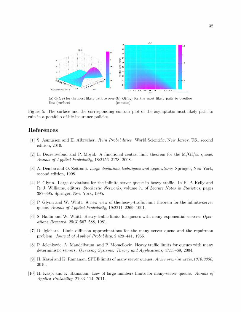
32

(a) Q(t, y) for the most likely path to over-flow (surface)

(b) Q(t, y) for the most likely path to overflow(contour)

Figure 5: The surface and the corresponding contour plot of the asymptotic most likely path toruin in a portfolio of life insurance policies.

References

[1] S. Asmussen and H. Albrecher. Ruin Probabilities. World Scientific, New Jersey, US., secondedition, 2010.

[2] L. Decreusefond and P. Moyal. A functional central limit theorem for the M/GI/∞ queue.Annals of Applied Probability, 18:2156–2178, 2008.

[3] A. Dembo and O. Zeitouni. Large deviations techniques and applications. Springer, New York,second edition, 1998.

[4] P. Glynn. Large deviations for the infinite server queue in heavy traffic. In F. P. Kelly andR. J. Williams, editors, Stochastic Networks, volume 71 of Lecture Notes in Statistics, pages387–395. Springer, New York, 1995.

[5] P. Glynn and W. Whitt. A new view of the heavy-traffic limit theorem for the infinite-serverqueue. Annals of Applied Probability, 19:2211–2269, 1991.

[6] S. Halfin and W. Whitt. Heavy-traffic limits for queues with many exponential servers. Oper-ations Research, 29(3):567–588, 1981.

[7] D. Iglehart. Limit diffusion approximations for the many server queue and the repairmanproblem. Journal of Applied Probability, 2:429–441, 1965.

[8] P. Jelenkovic, A. Mandelbaum, and P. Momcilovic. Heavy traffic limits for queues with manydeterministic servers. Queueing Systems: Theory and Applications, 47:53–69, 2004.

[9] H. Kaspi and K. Ramanan. SPDE limits of many server queues. Arxiv preprint arxiv:1010.0330,2010.

[10] H. Kaspi and K. Ramanan. Law of large numbers limits for many-server queues. Annals ofApplied Probability, 21:33–114, 2011.

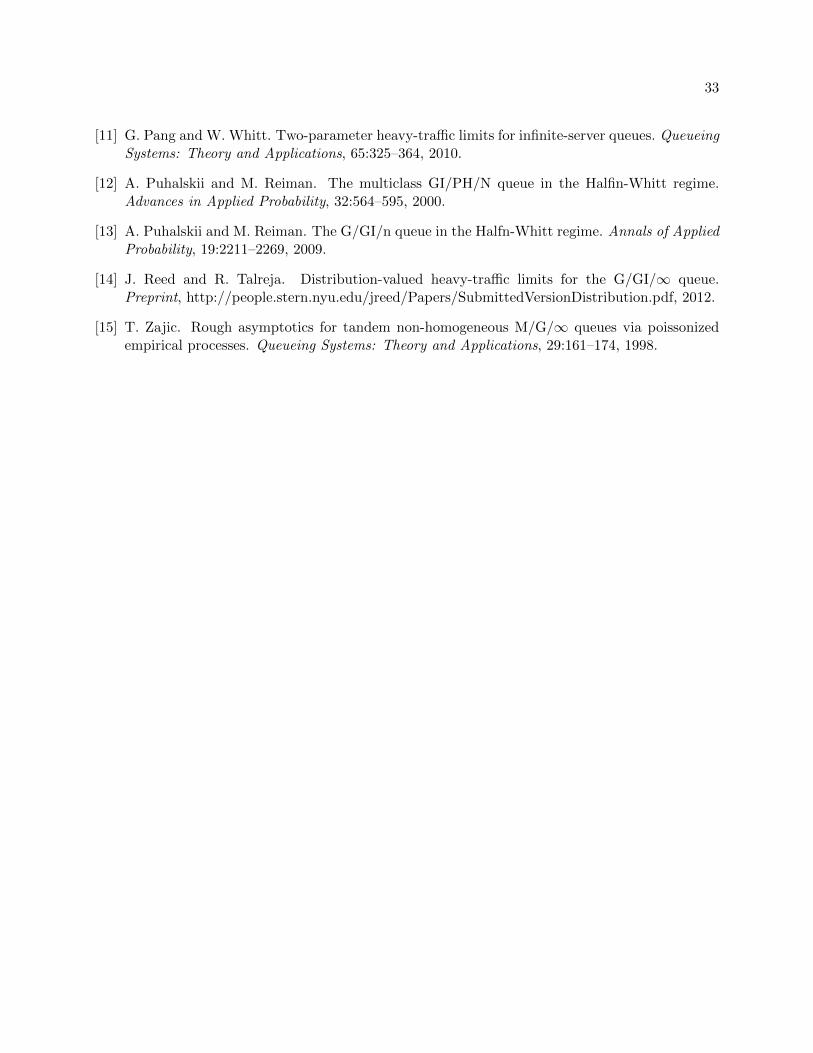
33

[11] G. Pang and W. Whitt. Two-parameter heavy-traffic limits for infinite-server queues. QueueingSystems: Theory and Applications, 65:325–364, 2010.

[12] A. Puhalskii and M. Reiman. The multiclass GI/PH/N queue in the Halfin-Whitt regime.Advances in Applied Probability, 32:564–595, 2000.

[13] A. Puhalskii and M. Reiman. The G/GI/n queue in the Halfn-Whitt regime. Annals of AppliedProbability, 19:2211–2269, 2009.

[14] J. Reed and R. Talreja. Distribution-valued heavy-traffic limits for the G/GI/∞ queue.Preprint, http://people.stern.nyu.edu/jreed/Papers/SubmittedVersionDistribution.pdf, 2012.

[15] T. Zajic. Rough asymptotics for tandem non-homogeneous M/G/∞ queues via poissonizedempirical processes. Queueing Systems: Theory and Applications, 29:161–174, 1998.