Bayesian Maximum Likelihood - Northwestern...
27
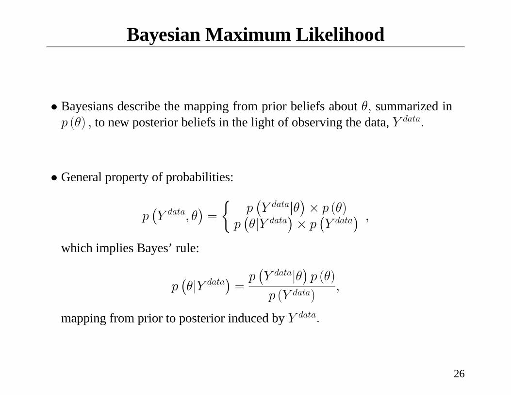
Bayesian Maximum Likelihood • Bayesians describe the mapping from prior beliefs about θ, summarized in p (θ ) , to new posterior beliefs in the light of observing the data, Y data . • General property of probabilities: p ¡ Y data ,θ ¢ = ½ p ¡ Y data |θ ¢ × p (θ ) p ¡ θ |Y data ¢ × p ¡ Y data ¢ , which implies Bayes’ rule: p ¡ θ |Y data ¢ = p ¡ Y data |θ ¢ p (θ ) p (Y data ) , mapping from prior to posterior induced by Y data . 26
-
Upload
truongtuong -
Category
Documents
-
view
226 -
download
0
Transcript of Bayesian Maximum Likelihood - Northwestern...
Bayesian Maximum Likelihood
• Bayesians describe the mapping from prior beliefs about θ, summarized inp (θ) , to new posterior beliefs in the light of observing the data, Y data.
• General property of probabilities:
p¡Y data, θ
¢=
½p¡Y data|θ
¢× p (θ)
p¡θ|Y data
¢× p
¡Y data
¢ ,
which implies Bayes’ rule:
p¡θ|Y data
¢=p¡Y data|θ
¢p (θ)
p (Y data),
mapping from prior to posterior induced by Y data.
26
Bayesian Maximum Likelihood ...
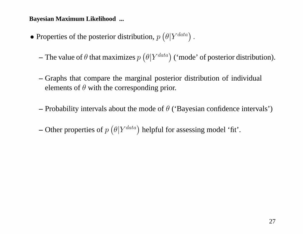
• Properties of the posterior distribution, p¡θ|Y data
¢.
– The value of θ that maximizes p¡θ|Y data
¢(‘mode’ of posterior distribution).
– Graphs that compare the marginal posterior distribution of individualelements of θ with the corresponding prior.
– Probability intervals about the mode of θ (‘Bayesian confidence intervals’)
– Other properties of p¡θ|Y data
¢helpful for assessing model ‘fit’.
27
Bayesian Maximum Likelihood ...
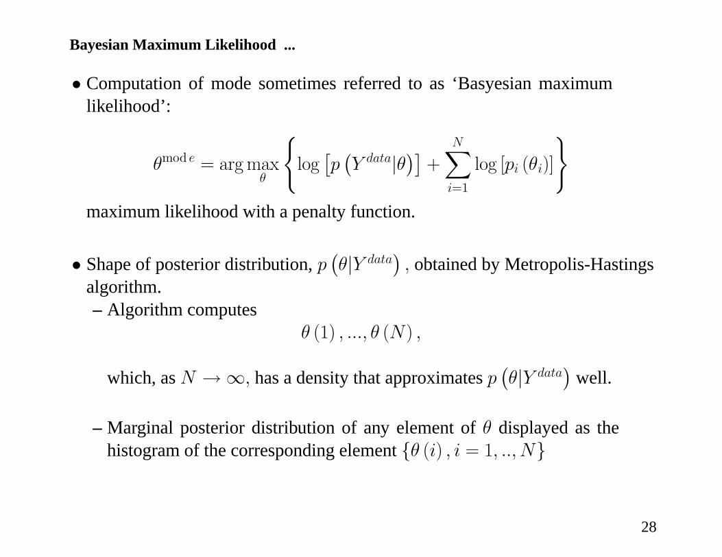
• Computation of mode sometimes referred to as ‘Basyesian maximumlikelihood’:
θmod e = argmaxθ
(log£p¡Y data|θ
¢¤+
NXi=1
log [pi (θi)]
)maximum likelihood with a penalty function.
• Shape of posterior distribution, p¡θ|Y data
¢, obtained by Metropolis-Hastings
algorithm.– Algorithm computes
θ (1) , ..., θ (N) ,
which, as N →∞, has a density that approximates p¡θ|Y data
¢well.
– Marginal posterior distribution of any element of θ displayed as thehistogram of the corresponding element {θ (i) , i = 1, .., N}
28
Metropolis-Hastings Algorithm (MCMC)
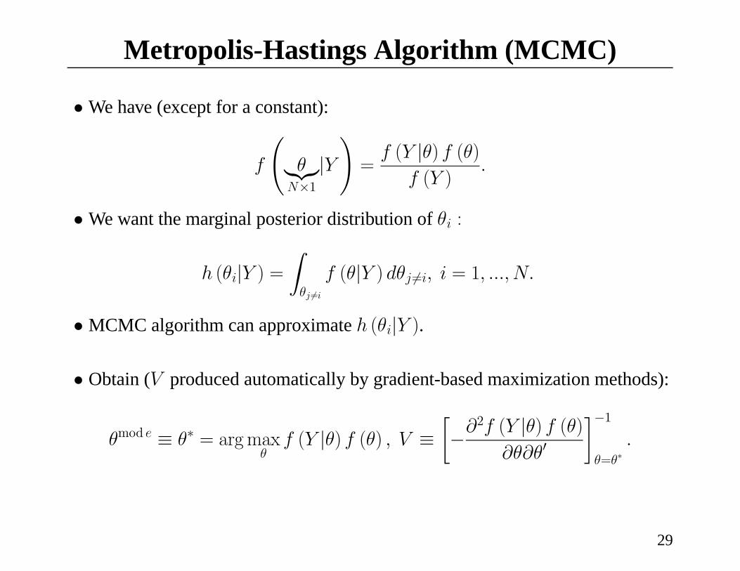
• We have (except for a constant):
f
Ãθ|{z}
N×1|Y!=f (Y |θ) f (θ)
f (Y ).
• We want the marginal posterior distribution of θi :
h (θi|Y ) =Zθj 6=i
f (θ|Y ) dθj 6=i, i = 1, ..., N.
• MCMC algorithm can approximate h (θi|Y ).
• Obtain (V produced automatically by gradient-based maximization methods):
θmod e ≡ θ∗ = argmaxθ
f (Y |θ) f (θ) , V ≡∙−∂
2f (Y |θ) f (θ)∂θ∂θ0
¸−1θ=θ∗
.
29
Metropolis-Hastings Algorithm (MCMC) ...
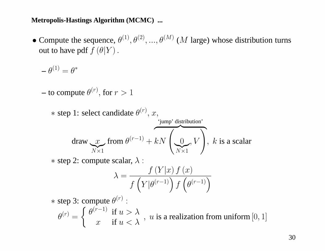
• Compute the sequence, θ(1), θ(2), ..., θ(M) (M large) whose distribution turnsout to have pdf f (θ|Y ) .
– θ(1) = θ∗
– to compute θ(r), for r > 1
∗ step 1: select candidate θ(r), x,
draw x|{z}N×1
from θ(r−1) +
‘jump’ distribution’z }| {kN
Ã0|{z}
N×1, V
!, k is a scalar
∗ step 2: compute scalar, λ :
λ =f (Y |x) f (x)
f³Y |θ(r−1)
´f³θ(r−1)
´∗ step 3: compute θ(r) :
θ(r) =
½θ(r−1) if u > λx if u < λ
, u is a realization from uniform [0, 1]
30
Metropolis-Hastings Algorithm (MCMC) ...
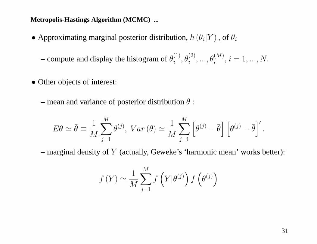
• Approximating marginal posterior distribution, h (θi|Y ) , of θi
– compute and display the histogram of θ(1)i , θ(2)i , ..., θ
(M)i , i = 1, ..., N.
• Other objects of interest:
– mean and variance of posterior distribution θ :
Eθ ' θ ≡ 1
M
MXj=1
θ(j), V ar (θ) ' 1
M
MXj=1
hθ(j) − θ
i hθ(j) − θ
i0.
– marginal density of Y (actually, Geweke’s ‘harmonic mean’ works better):
f (Y ) ' 1
M
MXj=1
f³Y |θ(j)
´f³θ(j)´
31
Larry Christiano
Text Box

Metropolis-Hastings Algorithm (MCMC) ...
• Some intuition
– Algorithm is more likely to select moves into high probability regions thaninto low probability regions.
– Set,nθ(1), θ(2), ..., θ(M)
o, populated relatively more by elements near mode
of f (θ|Y ) .
– Set,nθ(1), θ(2), ..., θ(M)
o, also populated (though less so) by elements far
from mode of f (θ|Y ) .
32
Metropolis-Hastings Algorithm (MCMC) ...
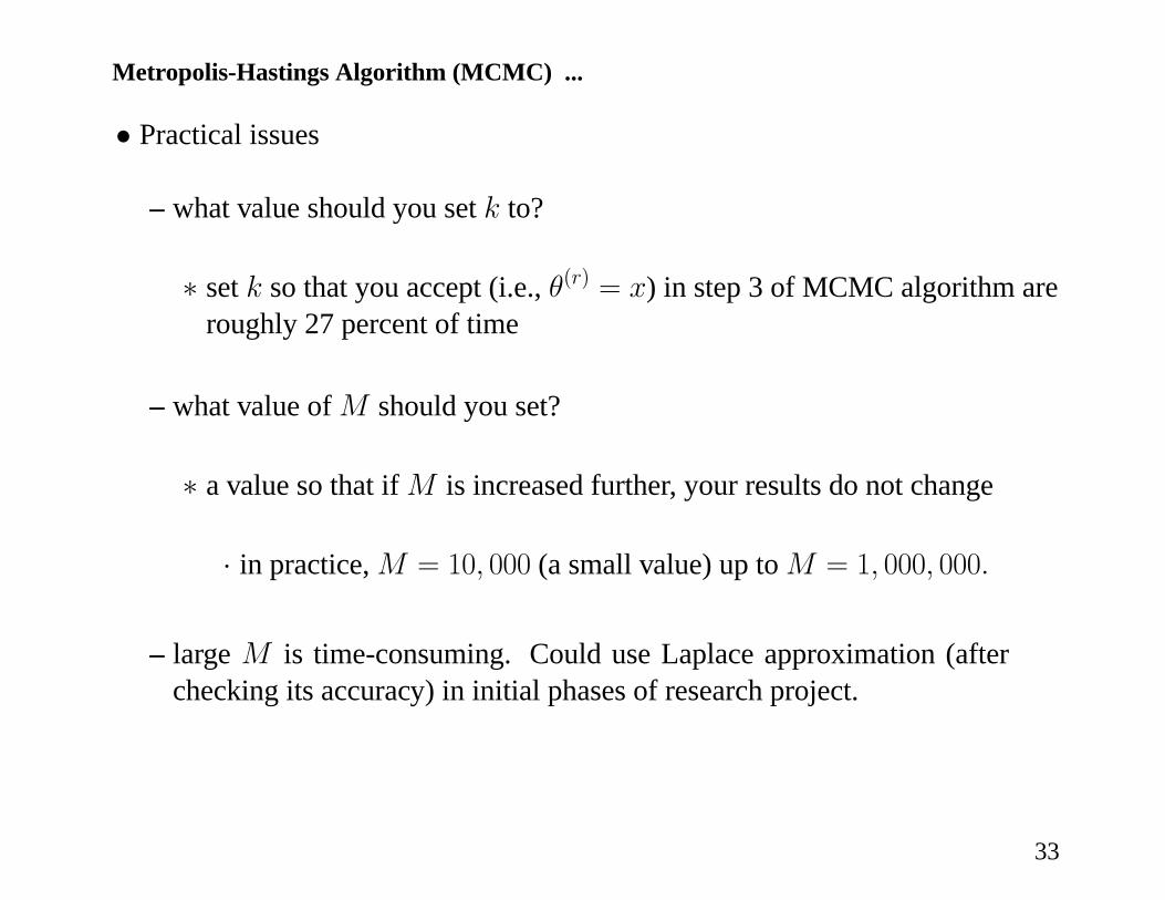
• Practical issues
– what value should you set k to?
∗ set k so that you accept (i.e., θ(r) = x) in step 3 of MCMC algorithm areroughly 27 percent of time
– what value of M should you set?
∗ a value so that if M is increased further, your results do not change
· in practice, M = 10, 000 (a small value) up to M = 1, 000, 000.
– large M is time-consuming. Could use Laplace approximation (afterchecking its accuracy) in initial phases of research project.
33
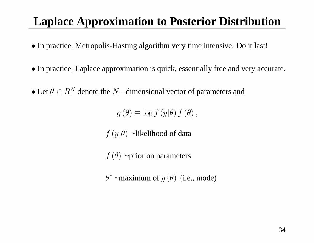
Laplace Approximation to Posterior Distribution
• In practice, Metropolis-Hasting algorithm very time intensive. Do it last!
• In practice, Laplace approximation is quick, essentially free and very accurate.
• Let θ ∈ RN denote the N−dimensional vector of parameters and
g (θ) ≡ log f (y|θ) f (θ) ,
f (y|θ) ~likelihood of data
f (θ) ~prior on parameters
θ∗ ~maximum of g (θ) (i.e., mode)
34
Laplace Approximation to Posterior Distribution ...
• Second order Taylor series expansion about θ = θ∗ :
g (θ) ≈ g (θ∗) + gθ (θ∗) (θ − θ∗)− 1
2(θ − θ∗)0 gθθ (θ
∗) (θ − θ∗) ,
where
gθθ (θ∗) = −∂
2 log f (y|θ) f (θ)∂θ∂θ0
|θ=θ∗
• Interior optimality implies:
gθ (θ∗) = 0, gθθ (θ
∗) positive definite
• Then,
f (y|θ) f (θ) ' f (y|θ∗) f (θ∗) exp½−12(θ − θ∗)0 gθθ (θ
∗) (θ − θ∗)
¾.
35
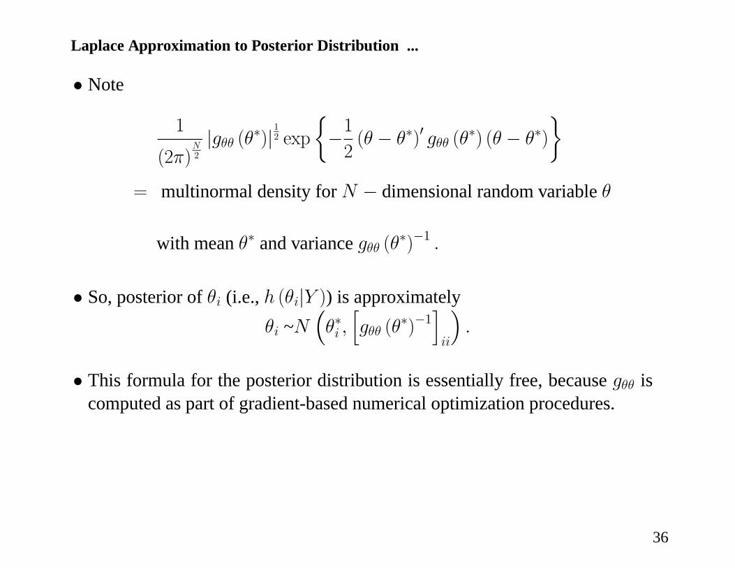
Laplace Approximation to Posterior Distribution ...
• Note
1
(2π)N2
|gθθ (θ∗)|12 exp
½−12(θ − θ∗)0 gθθ (θ
∗) (θ − θ∗)
¾= multinormal density for N − dimensional random variable θ
with mean θ∗ and variance gθθ (θ∗)−1 .
• So, posterior of θi (i.e., h (θi|Y )) is approximatelyθi ~N
³θ∗i ,hgθθ (θ
∗)−1iii
´.
• This formula for the posterior distribution is essentially free, because gθθ iscomputed as part of gradient-based numerical optimization procedures.
36
Laplace Approximation to Posterior Distribution ...
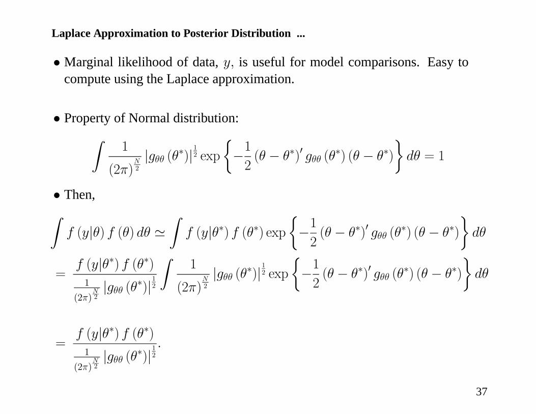
• Marginal likelihood of data, y, is useful for model comparisons. Easy tocompute using the Laplace approximation.
• Property of Normal distribution:Z1
(2π)N2
|gθθ (θ∗)|12 exp
½−12(θ − θ∗)0 gθθ (θ
∗) (θ − θ∗)
¾dθ = 1
• Then,Zf (y|θ) f (θ) dθ '
Zf (y|θ∗) f (θ∗) exp
½−12(θ − θ∗)0 gθθ (θ
∗) (θ − θ∗)
¾dθ
=f (y|θ∗) f (θ∗)1
(2π)N2|gθθ (θ∗)|
12
Z1
(2π)N2
|gθθ (θ∗)|12 exp
½−12(θ − θ∗)0 gθθ (θ
∗) (θ − θ∗)
¾dθ
=f (y|θ∗) f (θ∗)1
(2π)N2|gθθ (θ∗)|
12
.
37
Laplace Approximation to Posterior Distribution ...
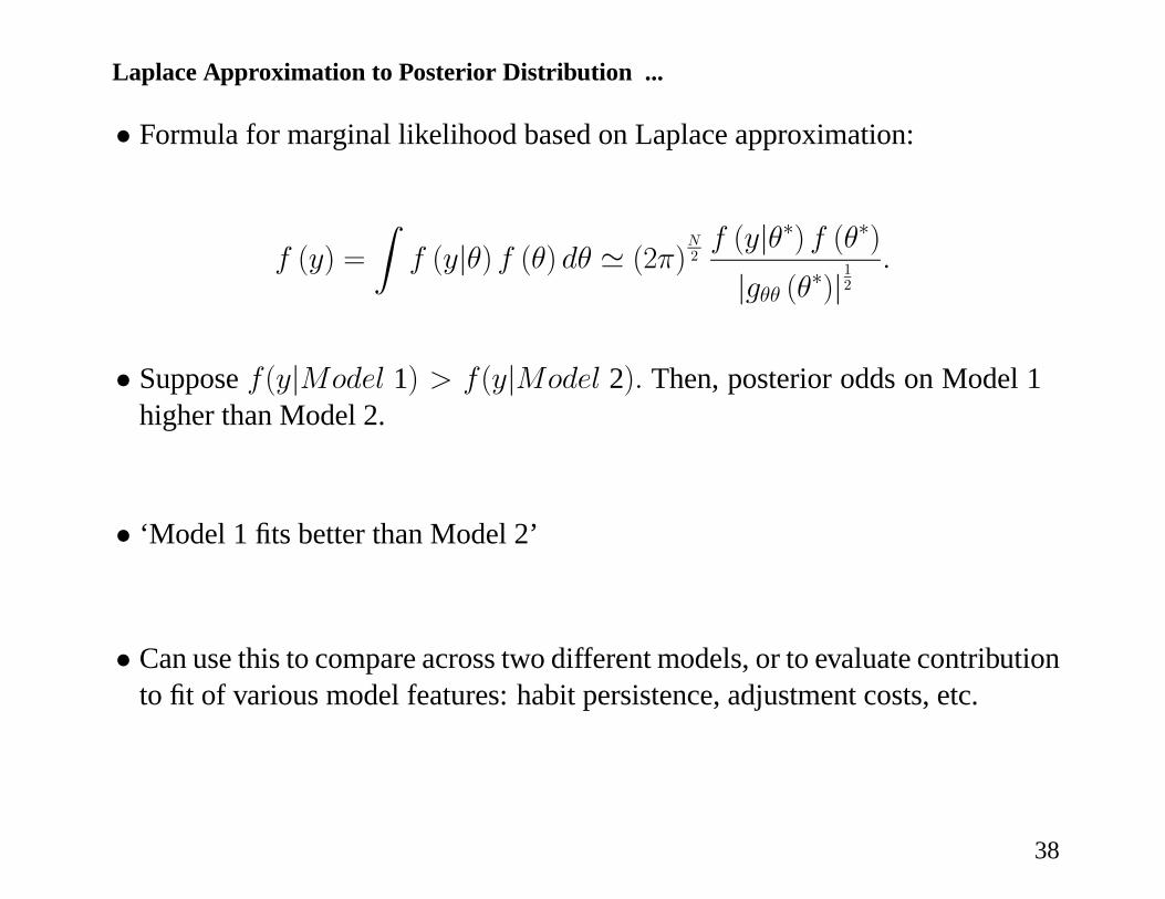
• Formula for marginal likelihood based on Laplace approximation:
f (y) =
Zf (y|θ) f (θ) dθ ' (2π)
N2f (y|θ∗) f (θ∗)|gθθ (θ∗)|
12
.
• Suppose f(y|Model 1) > f(y|Model 2). Then, posterior odds on Model 1higher than Model 2.
• ‘Model 1 fits better than Model 2’
• Can use this to compare across two different models, or to evaluate contributionto fit of various model features: habit persistence, adjustment costs, etc.
38
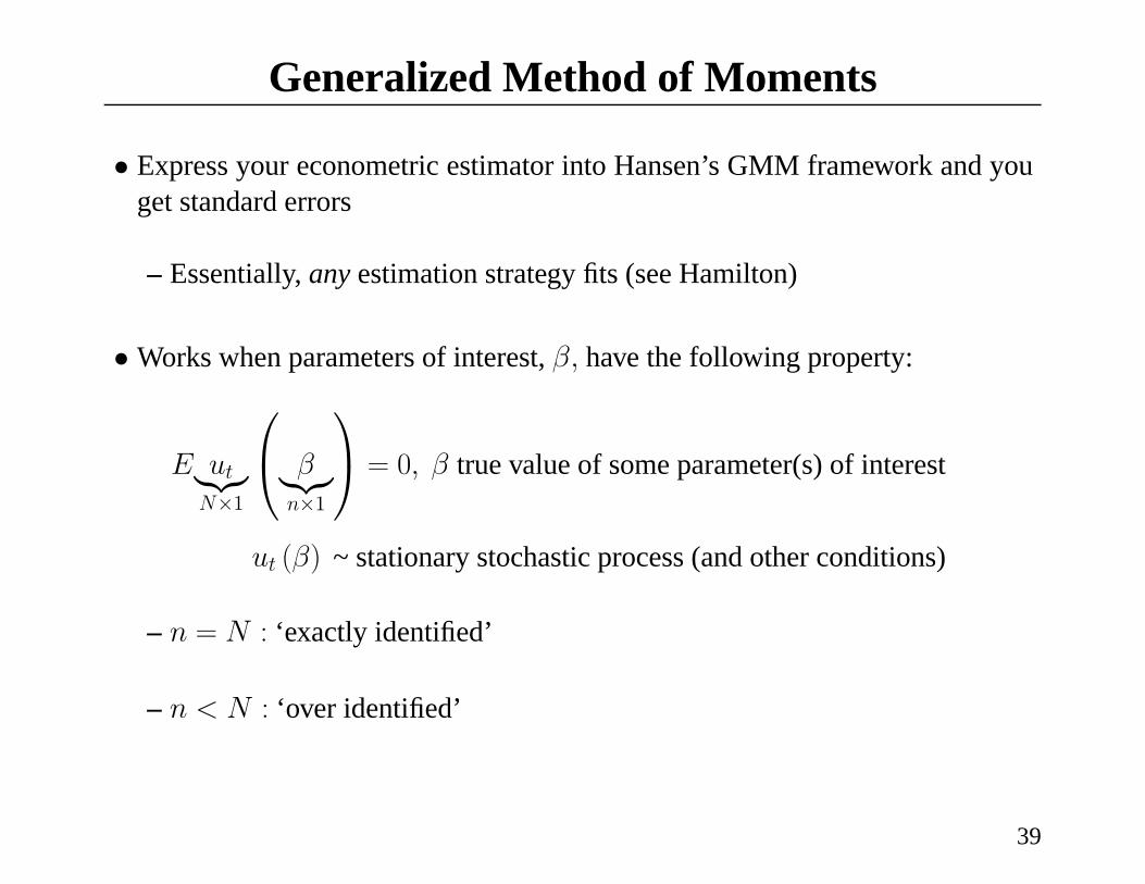
Generalized Method of Moments
• Express your econometric estimator into Hansen’s GMM framework and youget standard errors
– Essentially, any estimation strategy fits (see Hamilton)
• Works when parameters of interest, β, have the following property:
E ut|{z}N×1
⎛⎝ β|{z}n×1
⎞⎠ = 0, β true value of some parameter(s) of interest
ut (β) ~ stationary stochastic process (and other conditions)
– n = N : ‘exactly identified’
– n < N : ‘over identified’
39
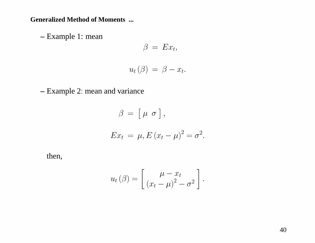
Generalized Method of Moments ...
– Example 1: meanβ = Ext,
ut (β) = β − xt.
– Example 2: mean and variance
β =£μ σ
¤,
Ext = μ,E (xt − μ)2 = σ2.
then,
ut (β) =
∙μ− xt
(xt − μ)2 − σ2
¸.
40
Generalized Method of Moments ...
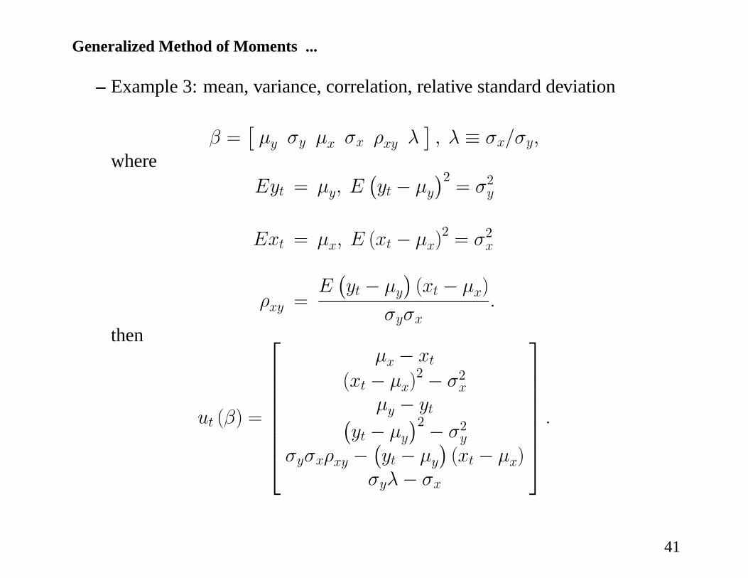
– Example 3: mean, variance, correlation, relative standard deviation
β =£μy σy μx σx ρxy λ
¤, λ ≡ σx/σy,
whereEyt = μy, E
¡yt − μy
¢2= σ2y
Ext = μx, E (xt − μx)2 = σ2x
ρxy =E¡yt − μy
¢(xt − μx)
σyσx.
then
ut (β) =
⎡⎢⎢⎢⎢⎢⎢⎢⎣
μx − xt(xt − μx)
2 − σ2xμy − yt¡
yt − μy¢2 − σ2y
σyσxρxy −¡yt − μy
¢(xt − μx)
σyλ− σx
⎤⎥⎥⎥⎥⎥⎥⎥⎦.
41
Generalized Method of Moments ...
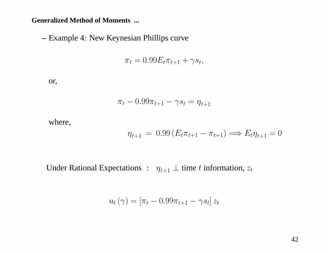
– Example 4: New Keynesian Phillips curve
πt = 0.99Etπt+1 + γst,
or,
πt − 0.99πt+1 − γst = ηt+1
where,ηt+1 = 0.99 (Etπt+1 − πt+1) =⇒ Etηt+1 = 0
Under Rational Expectations : ηt+1 ⊥ time t information, zt
ut (γ) = [πt − 0.99πt+1 − γst] zt
42
Generalized Method of Moments ...
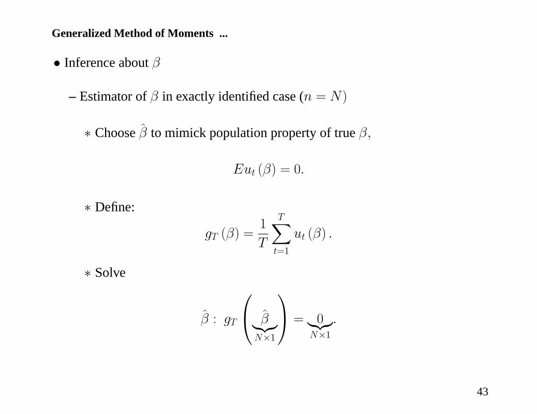
• Inference about β
– Estimator of β in exactly identified case (n = N)
∗ Choose β to mimick population property of true β,
Eut (β) = 0.
∗ Define:
gT (β) =1
T
TXt=1
ut (β) .
∗ Solve
β : gT
⎛⎝ β|{z}N×1
⎞⎠ = 0|{z}N×1
.
43
Generalized Method of Moments ...
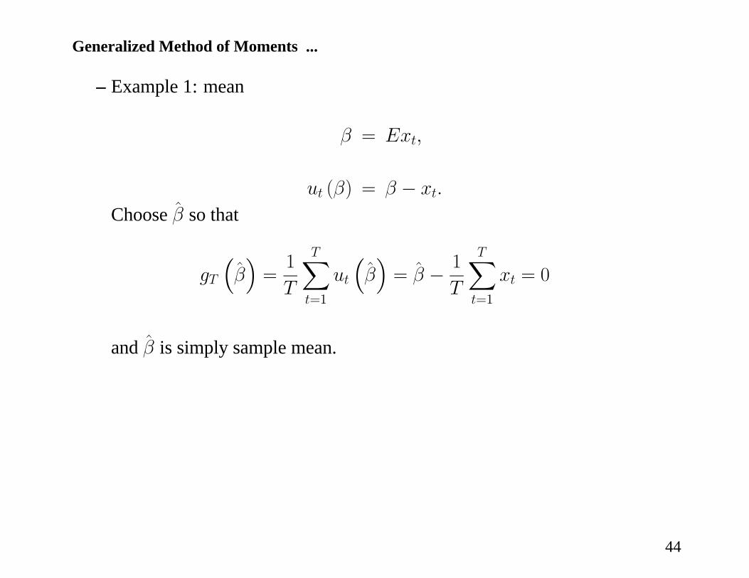
– Example 1: mean
β = Ext,
ut (β) = β − xt.
Choose β so that
gT
³β´=1
T
TXt=1
ut
³β´= β − 1
T
TXt=1
xt = 0
and β is simply sample mean.
44
Generalized Method of Moments ...
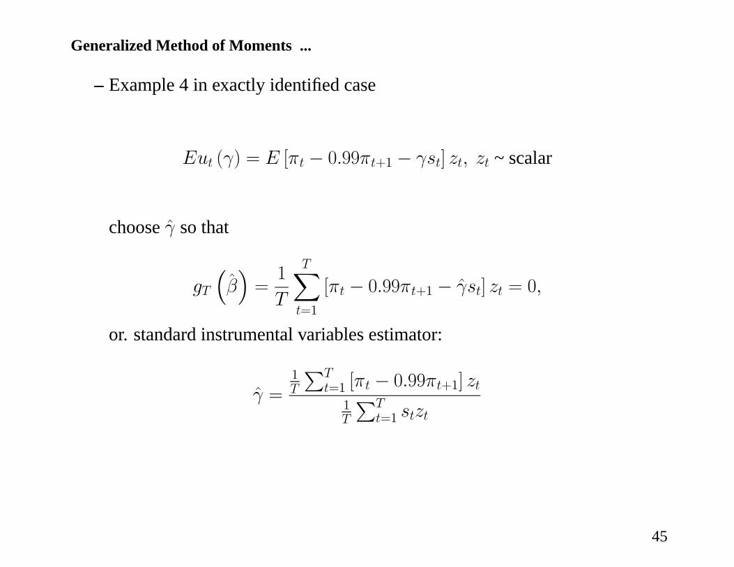
– Example 4 in exactly identified case
Eut (γ) = E [πt − 0.99πt+1 − γst] zt, zt ~ scalar
choose γ so that
gT
³β´=1
T
TXt=1
[πt − 0.99πt+1 − γst] zt = 0,
or. standard instrumental variables estimator:
γ =1T
PTt=1 [πt − 0.99πt+1] zt1T
PTt=1 stzt
45
Generalized Method of Moments ...
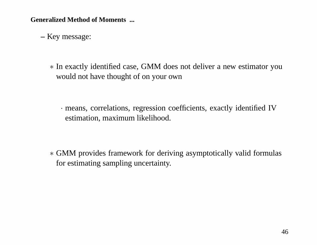
– Key message:
∗ In exactly identified case, GMM does not deliver a new estimator youwould not have thought of on your own
· means, correlations, regression coefficients, exactly identified IVestimation, maximum likelihood.
∗ GMM provides framework for deriving asymptotically valid formulasfor estimating sampling uncertainty.
46
Generalized Method of Moments ...
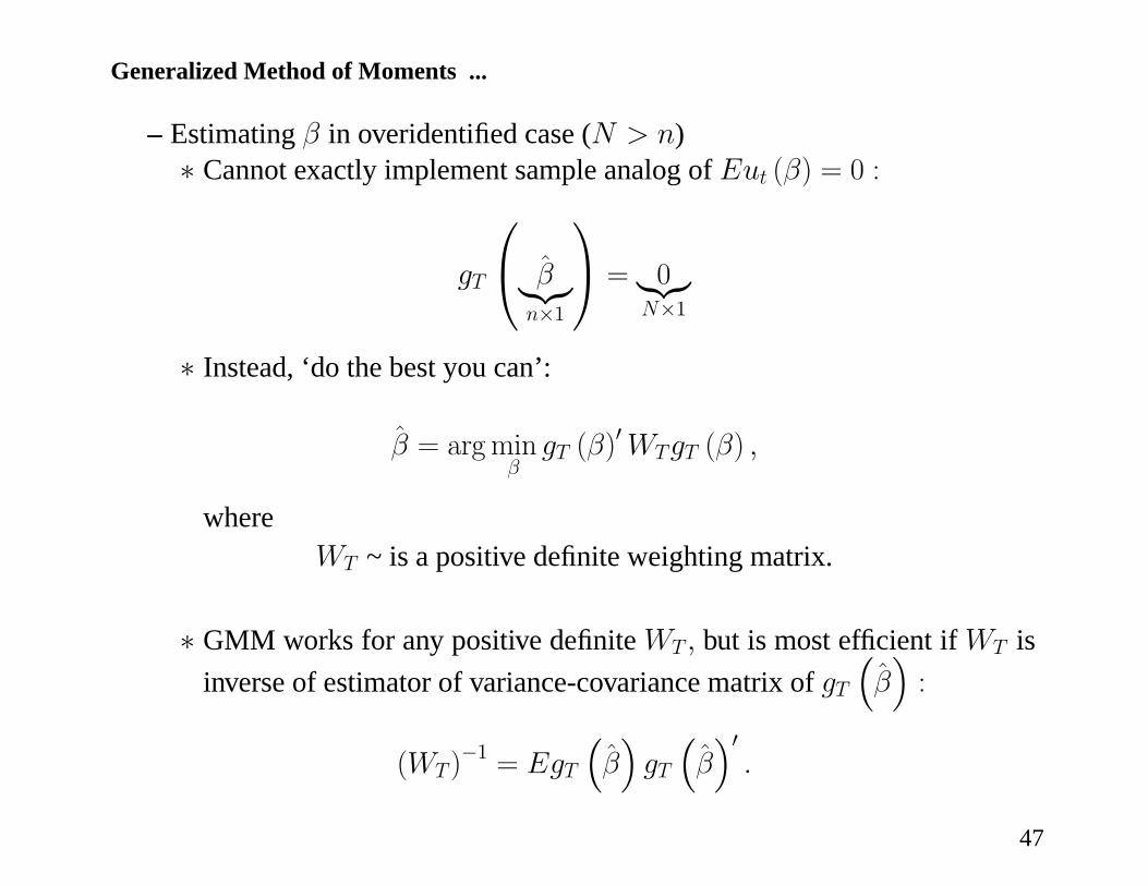
– Estimating β in overidentified case (N > n)∗ Cannot exactly implement sample analog of Eut (β) = 0 :
gT
⎛⎝ β|{z}n×1
⎞⎠ = 0|{z}N×1
∗ Instead, ‘do the best you can’:
β = argminβ
gT (β)0WTgT (β) ,
whereWT ~ is a positive definite weighting matrix.
∗ GMM works for any positive definite WT, but is most efficient if WT isinverse of estimator of variance-covariance matrix of gT
³β´:
(WT )−1 = EgT
³β´gT
³β´0.
47
Generalized Method of Moments ...
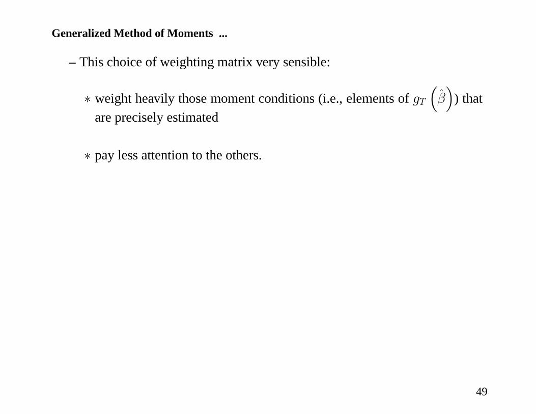
– This choice of weighting matrix very sensible:
∗ weight heavily those moment conditions (i.e., elements of gT³β´
) thatare precisely estimated
∗ pay less attention to the others.
49
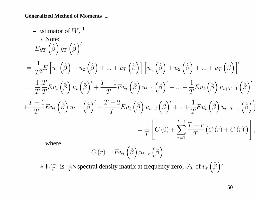
Generalized Method of Moments ...
– Estimator of W−1T
∗ Note:EgT
³β´gT
³β´0
=1
T 2Ehu1³β´+ u2
³β´+ ... + uT
³β´i h
u1³β´+ u2
³β´+ ... + uT
³β´i0
=1
T[T
TEut
³β´ut
³β´0+T − 1T
Eut
³β´ut+1
³β´0+ ... +
1
TEut
³β´ut+T−1
³β´0
+T − 1T
Eut
³β´ut−1
³β´0+T − 2T
Eut
³β´ut−2
³β´0+ .. +
1
TEut
³β´ut−T+1
³β´0]
=1
T
"C (0) +
T−1Xr=1
T − r
T
¡C (r) + C (r)0
¢#,
whereC (r) = Eut
³β´ut−r
³β´0
∗W−1T is ‘ 1T×spectral density matrix at frequency zero, S0, of ut
³β´
’
50
Generalized Method of Moments ...
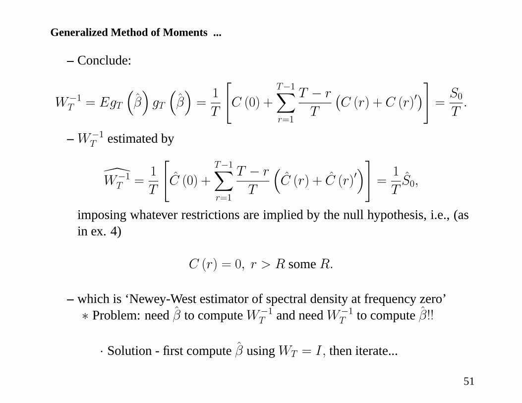
– Conclude:
W−1T = EgT
³β´gT
³β´=1
T
"C (0) +
T−1Xr=1
T − r
T
¡C (r) + C (r)0
¢#=S0T.
– W−1T estimated by
[W−1T =
1
T
"C (0) +
T−1Xr=1
T − r
T
³C (r) + C (r)0
´#=1
TS0,
imposing whatever restrictions are implied by the null hypothesis, i.e., (asin ex. 4)
C (r) = 0, r > R some R.
– which is ‘Newey-West estimator of spectral density at frequency zero’∗ Problem: need β to compute W−1
T and need W−1T to compute β!!
· Solution - first compute β using WT = I, then iterate...
51
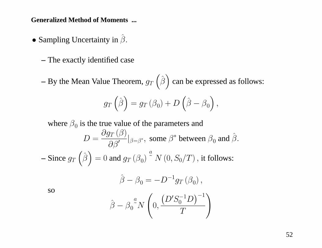
Generalized Method of Moments ...
• Sampling Uncertainty in β.
– The exactly identified case
– By the Mean Value Theorem, gT³β´
can be expressed as follows:
gT
³β´= gT (β0) +D
³β − β0
´,
where β0 is the true value of the parameters and
D =∂gT (β)
∂β0|β=β∗, some β∗ between β0 and β.
– Since gT³β´= 0 and gT (β0)
a˜ N (0, S0/T ) , it follows:
β − β0 = −D−1gT (β0) ,so
β − β0a˜N
Ã0,
¡D0S−10 D
¢−1T
!
52
Generalized Method of Moments ...
– The overidentified case.
∗ An extension of the ideas we have already discussed.
∗ Can derive the results for yourself, using the ‘delta function method’ forderiving the sampling distribution of statistics.
∗ Hamilton’s text book has a great review of GMM.
53