Recent advances on the inverse spectral problem

Steve ZelditchNorthwestern University

Joint work with Hamid Hezari (UC Irvine)

April 28, 2020

Can one hear the shape of a drum?

A drum (in this talk) is a smooth plane domain Ω ⊂ R2. A drumvibrates freely at its natural frequencies

√λj , which are the square

roots of the Dirichlet eigenvalues,

∆ϕ = −λϕ,

ϕ|∂Ω = 0.

There exists an orthonormal basis ϕΩj ∞j=1 of L2(Ω) of

eigenfunctions. The Laplace spectral map is the ordered list ofeigenvalues,

Λ(Ω) = (λΩ1 , λ

Ω2 , · · · , λΩ

n , . . . ).

Kac’s problem: Is Λ 1− 1 from the ‘space of domains’ to R∞+ ?

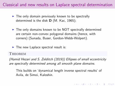
Classical and new results on Laplace spectral determination

I The only domain previously known to be spectrallydetermined is the disk D (M. Kac, 1965);

I The only domains known to be NOT spectrally determinedare certain non-convex polygonal domains (hence, withcorners) (Sunada, Buser, Gordon-Webb-Wolpert).

I The new Laplace spectral result is:

Theorem

(Hamid Hezari and S. Zelditch (2019)) Ellipses of small eccentricityare spectrally determined among all smooth plane domains.

This builds on ‘dynamical length inverse spectral results’ ofAvila, de Simoi, Kaloshin.

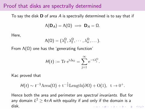
Proof that disks are spectrally determined

To say the disk D of area A is spectrally determined is to say that if

Λ(DA) = Λ(Ω) =⇒ DA = Ω.

Here,Λ(Ω) = (λΩ

1 , λΩ2 , · · · , λΩ

n , . . . ).

From Λ(Ω) one has the ‘generating function’

H(t) := Tr et∆Ω =∞∑

j=1

e−tλΩj .

Kac proved that

H(t) ∼ t−1Area(Ω) + t−12 Length(∂Ω) + O(1), t→ 0+.

Hence both the area and perimeter are spectral invariants. But forany domain L2 ≥ 4πA with equality if and only if the domain is adisk.

Quantum versus classical mechanics

Let Ee be an ellipse of eccentricity e. The proof of our main result,

Λ(Ω) = Λ(Ee) =⇒ Ω = Ee

is very different from Kac’. It is partly based on new results onbilliard dynamics, due to Avila, Kaloshin, de Simoi, Sorrentino, Weiand others on billiard dynamics.

The link between eigenvalues of ∆ (quantum mechanics) and

billiard dynamics is through the wave trace formula for Treit√−∆.

In addition to the billiard dynamics, the proof is based on veryspecial properties of the wave trace for any ‘nearly circular’ domainΩ. Only at the last step in the proof do we use that Ω isiso-spectral to Ee . There is potential for more general results.

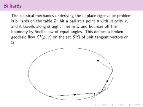
Billiards

The classical mechanics underlying the Laplace eigenvalue problemis billiards on the table Ω: hit a ball at a point p with velocity v ,and it travels along straight lines in Ω and bounces off theboundary by Snell’s law of equal angles. This defines a brokengeodesic flow G t(p, v) on the set S∗Ω of unit tangent vectors onΩ.

4 1 Aubry–Mather theory

h = h(x1 − x0),

with h′ = f−1; in other words, h is strictly convex.

Example 1.1.5. In some sense the “simplest” non–integrable monotone twistmap is the so–called standard map

φ : (x, y) "→(x + y +

k

2πsin 2πx, y +

k

2πsin 2πx

)

where k ≥ 0 is a parameter. This map has been the subject of extensiveanalytical and numerical studies. Famous pictures illustrate the transitionfrom integrability (k = 0) to “chaos” (k ≈ 10).

Example 1.1.6. A particularly interesting class of monotone twist maps comesfrom planar convex billiards; we will deal with convex billiards in Chap. 3.The investigation of such systems goes back to Birkhoff [15] who introducedthem as model case for nonlinear dynamical systems; for a modern survey see[101].

Fig. 1.2. The billard in a strictly convex domain

Given a strictly convex domain Ω in the Euclidean plane with smoothboundary ∂Ω, we play the following game. Let a mass point move freely insideΩ, starting at some initial point on the boundary with some initial directionpointing into Ω. When the “billiard ball” hits the boundary, it gets reflectedaccording to the rule “angle of incidence = angle of reflection”; see Fig. 1.2.The billiard map associates to a pair (point on the boundary, direction), re-spectively (s,ψ) = (arclength parameter divided by total length, angle withthe tangent), the corresponding data when the points hits the boundary again.The lift of this map, which is then defined on R × (0,π), is not a monotonetwist map.

Billiard map

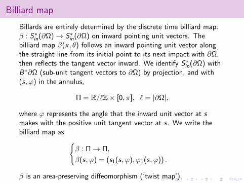
Billards are entirely determined by the discrete time billiard map:β : S∗in(∂Ω)→ S∗in(∂Ω) on inward pointing unit vectors. Thebilliard map β(x , θ) follows an inward pointing unit vector alongthe straight line from its initial point to its next impact with ∂Ω,then reflects the tangent vector inward. We identify S∗in(∂Ω) withB∗∂Ω (sub-unit tangent vectors to ∂Ω) by projection, and with(s, ϕ) in the annulus,

Π = R/`Z× [0, π], ` = |∂Ω|,

where ϕ represents the angle that the inward unit vector at smakes with the positive unit tangent vector at s. We write thebilliard map as

β : Π→ Π,

β(s, ϕ) = (s1(s, ϕ), ϕ1(s, ϕ)) .

β is an area-preserving diffeomorphism (‘twist map’).

Caustics and Invariant curves

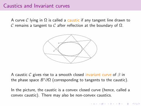
A curve C lying in Ω is called a caustic if any tangent line drawn toC remains a tangent to C after reflection at the boundary of Ω.

3.1 Convex billiards 41

ML(Ω) : Q ∩(0,

1

2

]→ R

that associates to any m/n in lowest terms the maximal length of closedgeodesics having rotation number m/n.

The length spectrum of Ω is defined as the set

L(Ω) := N lengths of closed geodesics in Ω ∪ N l(∂Ω).

Note that, due to Birkhoff’s theorem, the marked length spectrum is awell defined map. Moreover, l(∂Ω) = 1 by our standing assumption that theboundary length is normalized to 1.

The length spectrum contains information about all closed geodesics, al-beit in an “unformatted” form. In contrast, the marked length spectrum doesgive the labelling by the rotation number but only for the closed geodesics ofmaximal length.

Have you ever visited the great basilica in Rome and stood in its huge dome(42m in diameter)? If you are inside the domed roof and try to communicatewith a friend on the other side of the dome. Rather than shouting into the air,get close to the circular wall and whisper along the wall – you will be heardclearly on the other side.

This is the effect of what is usually called a “whispering gallery”. Thesound waves get reflected and travel along the wall, always staying close to it.In the context of billiards, such a whispering gallery is called a caustic.

Fig. 3.3. A convex caustic

Definition 3.1.5. Let Ω be a strictly convex bounded domain in R2. A convexcaustic is a closed C1–curve in the interior of Ω, bounding itself a strictlyconvex domain, with the property that each trajectory that is tangent to itstays tangent after each reflection; see Fig. 3.3.

A caustic C gives rise to a smooth closed invariant curve of β inthe phase space B∗∂Ω (corresponding to tangents to the caustic).

In the picture, the caustic is a convex closed curve (hence, called aconvex caustic). There may also be non-convex caustics.

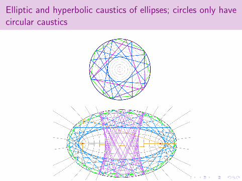
Elliptic and hyperbolic caustics of ellipses; circles only havecircular caustics

COMPUTING MATHER’S -FUNCTION FOR BIRKHOFF BILLIARDS 5059

In particular, stays constant along the orbit and it represents an integral of motionfor the map. Moreover, this billiard enjoys the peculiar property of having the phasespace – which is topologically a cylinder – completely foliated by homotopicallynon-trivial invariant curves C0 = 0. These curves correspond to concentriccircles of radii 0 = R cos 0 and are examples of what are called caustics, i.e.,(smooth and convex) curves with the property that if a trajectory is tangent to oneof them, then it will remain tangent after each reflection (see figure 2).

Figure 2. Billiard in a disc

A billiard in a disc is an example of an integrable billiard. There are di↵erent waysto define global/local integrability for billiards (the equivalence of these notions isan interesting problem itself):

- either through the existence of an integral of motion, globally or locally nearthe boundary (in the circular case an integral of motion is given by I(s, ) = ),

- or through the existence of a (smooth) foliation of the whole phase space (orlocally in a neighbourhood of the boundary = 0), consisting of invariantcurves of the billiard map; for example, in the circular case these are given byC. This property translates (under suitable assumptions) into the existenceof a (smooth) family of caustics, globally or locally near the boundary (in thecircular case, the concentric circles of radii R cos ).

In [2], Misha Bialy proved the following beautiful result concerning global inte-grability (see also [24]):

Theorem (Bialy). If the phase space of the billiard ball map is globally foliatedby continuous invariant curves which are not null-homotopic, then it is a circularbilliard.

However, while circular billiards are the only examples of global integrable bil-liards, local integrability is still an intriguing open question. One could consider abilliard in an ellipse: this is in fact (locally) integrable (see Section 3.2). Yet, thedynamical picture is very distinct from the circular case: as it is showed in figure3, each trajectory which does not pass through a focal point, is always tangent toprecisely one confocal conic section, either a confocal ellipse or the two branches ofa confocal hyperbola (see for example [22, Chapter 4]). Thus, the confocal ellipsesinside an elliptical billiards are convex caustics, but they do not foliate the whole

5060 ALFONSO SORRENTINO

domain: the segment between the two foci is left out (describing the dynamicsexplicitly is much more complicated: see for example [23] and Section 3.2).

Figure 3. Billiard in an ellipse

Question II (Birkho↵). Are there other examples of (locally) integrable billiards?

A negative answer to this question would solve what is generally known asBirkho↵ conjecture: amongst all convex billiards, the only integrable ones are theones in ellipses (a circle is a distinct special case).

Despite its long history and the amount of attention that this conjecture has cap-tured, it remains essentially open. As far as our understanding of integrable billiardsis concerned, the two most important related results are the above–mentioned the-orem by Bialy [2] (see also [24]), a result by Delshams and Ramırez-Ros [5] in whichthey study entire perturbations of elliptic billiards and prove that any nontrivialsymmetric perturbation of the elliptic billiard is not integrable, and a theorem byMather [13] which proves the non-existence of caustics (hence, the non-integrability)if the curvature of the boundary vanishes at one point. This latter justifies the re-striction of our attention to strictly convex domains.

We shall see in the next subsection how this conjecture/question can be rephrasedas a regularity question for Mather’s function (see Question II bis).

1.3 - Mather’s minimal average action (or -function) and billiards.At the beginning of the eighties Serge Aubry and John Mather developed, in-

dependently, what nowadays is commonly called Aubry–Mather theory. This novelapproach to the study of the dynamics of twist di↵eomorphisms of the annulus,pointed out the existence of many action-minimizing orbits for any given rotationnumber (for a more detailed introduction, see for example [15, 19, 20]).

More precisely, let f : R/Z R ! R/Z R a monotone twist map, i.e., a

C1 di↵eomorphism such that its lift to the universal cover f satisfies the followingproperties (we denote (x1, y1) = f(x0, y0)):

(i) f(x0 + 1, y0) = f(x0, y0) + (1, 0),(ii) @x1

@y0> 0 (monotone twist condition),

(iii) f admits a (periodic) generating function h (i.e., it is an exact symplecticmap):

y1 dx1 y0 dx0 = dh(x0, x1).

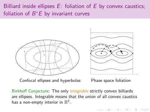
Billiard inside ellipses E : foliation of E by convex caustics;foliation of B∗E by invariant curves

3.1 Convex billiards 43

which case the trajectory never intersects the segment between the foci) orthe two branches of a confocal hyperbola (where the trajectory always in-tersects the segment between the foci); see Fig. 3.5. The eccentricity of thecorresponding conic section, for example, can be taken as an integral for theelliptical billiard. For proofs and further remarks, the reader may consult[24, 101].

Thus, the confocal ellipses inside an elliptical billiard are convex causticsin accordance with Def. 3.1.5, so the elliptical billiard is foliated by convexcaustics (up to the segment between the foci). The branches of the confocalhyperbolae can then be seen as caustics in the more general sense mentionedabove.

(a) Caustics are confocal ellipses and hy-perbolae

x

y

(b) Phase portrait

Fig. 3.5. The billiard inside an ellipse

The phase portrait of an elliptical billiard is also shown in Fig. 3.5. Al-though it looks like the phase portrait of the pendulum (Fig. 1.3), the dynam-ics are quite different. The points (0, 0) and (1/2, 0) and its translates do notrepresent equilibrium points anymore, but belong to the two–periodic orbitscorresponding one of the half–axes of the ellipse, and similarly for the otherhalf–axis. Their rotation number is 1/2, which implies that the islands are notfixed, but “wander”: they are mapped onto each other.

Bounding the islands we see separatrices, corresponding to the orbitsthrough the foci. The invariant curves above and below the seperatrices rep-resent the orbits not intersecting the segment between the foci (i.e., beingtangent to confocal hyperbola).

As an aside, we mention here that a famous conjecture, usually attributedto Birkhoff, states that the elliptical is, in fact, the only convex billiard withan integral.

Confocal ellipses and hyperbolas Phase space foliation

Birkhoff Conjecture: The only integrable strictly convex billiardsare ellipses. Integrable means that the union of all convex causticshas a non-empty interior in R2.

Phase space portraitThe frequency map for billiards inside ellipsoids 14

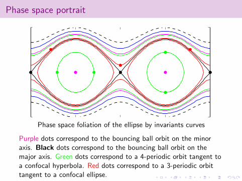
Figure 1. Phase portrait of the billiard map in (', r) coordinates for a = 1 and b = 4/9.The dashed black lines enclose the phase space (10). The black points are the hyperbolic two-periodic points corresponding to the oscillation along the major axis of the ellipse. The blackcurves are the separatrices of these hyperbolic points. The magenta points denote the elliptictwo-periodic points corresponding to the oscillation along the minor axis of the ellipse. Themagenta curves are the invariant curves whose rotation number coincides with the frequencyof these elliptic points. The invariant curves with rotation numbers 1/6, 1/4 and 1/3 aredepicted in blue, green and red, respectively. The red points label a three-periodic trajectorywhose caustic is an ellipse. The green points label a four-periodic trajectory whose caustic isa hyperbola.

4.3. Analytical properties of the rotation number

Let () be the rotation number of the billiard trajectories inside the ellipse Q sharing thenonsingular caustic Q. From definition 2 we get that the function : E [ H ! R is givenby the quotients of elliptic integrals

() = (; b, a) =

R min(b,)

0dsp

(s)(bs)(as)

2R a

max(b,)dsp

(s)(bs)(as)

=

R µ

dtp

t(t1)(t)

2R 1

0dtp

t(t1)(t)

, (11)

where the parameters 1 < < µ are given by = (a m)/(a m) and µ = a/(a m),with m = min(b,) and m = max(b,). The second equality follows from the change ofvariables t = (a s)/(am). The second quotient already appears in [12]. Other equivalentquotients of elliptic integrals were given in [30, 41]. We have drawn the rotation function ()

in figure 2, compare with [41, figure 2].

Proposition 8. The function : E [ H ! R given in (11) has the following properties.

(i) It is analytic in = E [ H and increasing in E.

Phase space foliation of the ellipse by invariants curves

Purple dots correspond to the bouncing ball orbit on the minoraxis. Black dots correspond to the bouncing ball orbit on themajor axis. Green dots correspond to a 4-periodic orbit tangent toa confocal hyperbola. Red dots correspond to a 3-periodic orbittangent to a confocal ellipse.

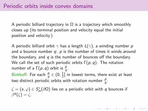
Periodic orbits inside convex domains

A periodic billiard trajectory in Ω is a trajectory which smoothlycloses up (its terminal position and velocity equal the initialposition and velocity.)

A periodic billiard orbit γ has a length L(γ), a winding number pand a bounce number q: p is the number of times it winds aroundthe boundary, and q is the number of bounces off the boundary.We call the set of such periodic orbits Γ(p, q). The rotationnumber of a Γ(p, q) orbit is p

q .

Birkhoff: For each pq ∈ (0, 1

2 ] in lowest terms, there exist at least

two distinct periodic orbits with rotation number pq .

ζ = (s, ϕ) ∈ S∗in(∂Ω) lies on a periodic orbit with q bounces ifβq(ζ) = ζ.

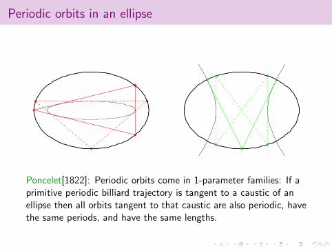
Periodic orbits in an ellipse

The frequency map for billiards inside ellipsoids 18

Figure 3. Examples of symmetric nonsingular billiard trajectories with minimal periods fora = 1 and b = 4/9. Left: Period three and the caustic is an ellipse. Right: Period four and thecaustic is a hyperbola. The continuous lines are reserved for the trajectories that correspond tothe periodic orbits depicted in figure 1.

Proposition 11.1.8]. Since the underlying idea is the same, we have preferred our geometricfinite argument.

Unfortunately, neither the geometric argument nor the dynamical approach based ontwist maps have a clear correspondence when the caustics are hyperbolas. The main problemis that when 2 H the invariant curves in the phase space (10) are not projected one-to-oneonto the configuration space T = Q. On the other hand, the obvious computational approach—to check that the derivative of the quotient of elliptic integrals (11) is negative for 2 H—becomes too cumbersome. Thus, although we have no doubt that the rotation number isdecreasing in H , we have failed to prove it or to find a proof in the literature.

4.5. Bifurcations in parameter space

We want to determine the ellipses that have billiard trajectories with a prescribed rotationnumber and with a prescribed type of caustics (ellipses or hyperbolae). We recall that therotation function () maps E onto (0, 1/2), and H onto (, 1/2). Therefore, once prescribedany rotation number 0 2 (0, 1/2), we can always find an ellipse as caustic with that number,whereas a such hyperbola only exists when 0 > ; that is, when b < a sin2 0. This showsthat flat ellipses have more periodic trajectories than rounded ones. There exists similar resultsfor triaxial ellipsids of R3; see section 5.4.

4.6. Examples of periodic trajectories with minimal periods

If n = 1, the function : 0, 1n ! n + 2, . . . , 2n + 2 defined in theorem 7 reduces to

(0) = 3, (1) = 4.

We also recall that the two connected components of are 0 = E and 1 = H . Therefore,the lower bounds established in theorem 7 imply that the periodic trajectories with an ellipse

Poncelet[1822]: Periodic orbits come in 1-parameter families: If aprimitive periodic billiard trajectory is tangent to a caustic of anellipse then all orbits tangent to that caustic are also periodic, havethe same periods, and have the same lengths.

Circular domains (disk)

A billiard trajectory of the disk is determined by the angle θ itmakes with the circle. The angle remains the same after eachreflection.If θ = p

q then the billiard orbit with this angle is periodicof period q and makes p turns around the boundary.

I A Γ(1, q) orbit is a regular q-gon (The angles are the same atall q bounce points).

I The length of a Γ(1, q) orbit is 2q sin πq .

I The rotate of a periodic orbit is periodic: periodic orbits comein circular families.

Question: What happens if we perturb the disk?

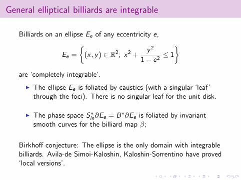
General elliptical billiards are integrable

Billiards on an ellipse Ee of any eccentricity e,

Ee =

(x , y) ∈ R2; x2 +

y2

1− e2≤ 1

are ‘completely integrable’.

I The ellipse Ee is foliated by caustics (with a singular ‘leaf’through the foci). There is no singular leaf for the unit disk.

I The phase space S∗in∂Ee = B∗∂Ee is foliated by invariantsmooth curves for the billiard map β;

Birkhoff conjecture: The ellipse is the only domain with integrablebilliards. Avila-de Simoi-Kaloshin, Kaloshin-Sorrentino have proved‘local versions’.

Rationally integrable

Definition:(i) An integrable rational caustic Γ ⊂ Ω is a caustic such thattangential orbits are periodic. The corresponding(non-contractible) invariant curve in B∗∂Ω = Π consists ofperiodic points (hence the rotation number is rational).

(ii) Ω is rationally integrable if the billiard map of Ω admitsintegrable rational caustics of rotation number 1

q for all q ≥ 3.

Rationally integrable is weaker than integrability: one does not usea foliation by caustics or invariant curves, but only a ‘partial,rational, foliation’ by invariant curves of periodic points.

Rigidity of ellipses

Birkhoff Conjecture: The only integrable strictly convex billiardsare ellipses. Integrable means that the union of all convex causticshas a non-empty interior in R2.

Avila-De Simoi-Kaloshin[15]: A rationally integrable billiard tablewhich is nearly circular must be an ellipse.

Kaloshin-Sorrentino[17]: A rationally integrable billiard table whichis sufficiently close to an ellipse must be an ellipse.

This is good news for ∆-spectral analysts, because the ∆-spectrumonly ‘sees’ periodic orbits.

Deformations (perturbations) of a domain

Inverse results are often based on perturbation theory of domains.If Ω is a domain, we perturb it by deforming the boundary:

∂Ω→ ∂Ω + ε~n

where ~n(x) = ρ(x)ν(x) is a multiple ρ(x) of the unit normal ν(x)at x ∈ ∂Ω.

I (Ramirez-Ros) If the foliation by caustics of D persists underperturbation ∂D + ε~n, then ~n is trivial. Proof: study theFourier coefficients of ~n; they must be trivial.

I (Avila-de Simoi-Kaloshin) For ellipses of small eccentricity, ifrational caustics persist under perturbation, then theperturbation is trivial. Proof: construct a good basis like sinesand cosines on ∂Ω and prove orthogonality relations for ~n.

I A domain is δ-nearly circular if ∂Ω = ∂D + ~n where ~n and 39of its derivatives are < δ.

Laplace spectral rigidity of ellipses

One can also study perturbations of eigenvalues.Hezari.- Z[2012]: Ellipses are infinitesimally spectrally rigid amongsmooth domains with the Z2 × Z2 reflectional symmetries of theellipse.

Popov-Topalov[2016]: Analogous result holds for ellipsoids in R3.

The new result uses geometric perturbation theory:

Theorem

(Hamid Hezari and S. Zelditch (2019)) Ellipses of small eccentricityare spectrally determined among all smooth plane domains.

The proof uses very special properties of the ‘length spectrum’ andthe ‘wave trace’ of a nearly circular domain.

Length spectrum for nearly circular billiards

The length spectrum is the set of lengths of closed billiardtrajectories,

Lsp(Ω) = L ∈ R : ∃ periodic γ : L(γ) = L.

Let Γ(p, q) be the periodic orbits with winding number p andbounce number q. Let LΓ(p, q) be the lengths L(γ) of the periodicorbits γ ∈ Γ(p, q).

We are mainly concerned with Γ(1, q) orbits. For a nearly-circulardomain, only these orbits have lengths < |∂Ω|. Let

tq = infγ∈Γ(1,q)

L(γ), Tq = supγ∈Γ(1,q)

L(γ).

Length spectrum and the band-gap property for nearlycircular billiards

The length spectrum is the set of lengths of closed billiardtrajectories,

Lsp(Ω) = L ∈ R : ∃ periodic γ : Lγ = L.

BAND-GAP property of nearly-circular domains (` = |∂Ω|):

Lsp(Ω) ∩ [0, `] =⋃

q≥2

LΓ(1, q) ⊂⋃

q≥2

[tq,Tq]

where the band = interval [tq,Tq] contains the lengths of Γ(1, q)periodic orbits with q bounces. The gaps Tq+1 − tq ∼ q−3 areMUCH bigger than the bands Tq − tq ∼ q−∞: the bounce numberq is determined by the length of the orbit.Prior results: Marvizi-Melrose (did q ≥ q0(Ω)).

More details on Band-gap property for nearly circularbilliards

Let ∂Ωτ = ∂E0 + τ fN0 be a curve of nearly circular domains. Weneed dependence of estimates [tq,Tq] = O(q−∞) >> gapstq+1 − Tq ∼ q3, on f :

Assume ‖f ‖C8 ≤ 1 and ‖f ‖C2 is sufficiently small so thatκτ = 1 + O(‖f ‖C2) ≥ 1

2 . Then,

Tq − tq = q−3O(‖f ‖C6) + O(q−4), (1)

Tq = `τ−1

4

(∫ `τ

0κ2/3τ (s) ds

)3

q−2+q−3O(‖f ‖C6)+O(q−4). (2)

Wave trace approach (Poisson relation)

The inverse spectral results are based on the trace of the wavegroup U(t) = e it

√−∆ of on L2(Ω). The wave trace is,

TrU(t) =∑

λj∈Sp(−∆)

e it√λj .

It is a tempered distribution on R, which is smooth except whent ∈ ±Lsp(Ω) ∪ 0, where

Lsp(Ω) = L ∈ R : ∃ periodic γ : L(γ) = L.Note: ⋃

q≥2

LΓ(1, q) = Lsp(Ω) ∩ [0, |∂Ω|].

Theorem (Hezari-Z)

For a nearly circular domain, TrU(t) determines the entire⋃q≥2 LΓ(1, q). Moreover, it determines bounce numbers for each

length.

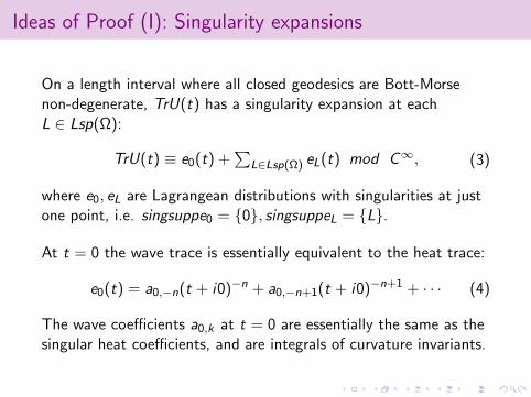
Ideas of Proof (I): Singularity expansions

On a length interval where all closed geodesics are Bott-Morsenon-degenerate, TrU(t) has a singularity expansion at eachL ∈ Lsp(Ω):

TrU(t) ≡ e0(t) +∑

L∈Lsp(Ω) eL(t) mod C∞, (3)

where e0, eL are Lagrangean distributions with singularities at justone point, i.e. singsuppe0 = 0, singsuppeL = L.

At t = 0 the wave trace is essentially equivalent to the heat trace:

e0(t) = a0,−n(t + i0)−n + a0,−n+1(t + i0)−n+1 + · · · (4)

The wave coefficients a0,k at t = 0 are essentially the same as thesingular heat coefficients, and are integrals of curvature invariants.

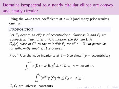
Domains isospectral to a nearly circular ellipse are convexand nearly circular

Using the wave trace coefficients at t = 0 (and many prior results),one has:

Proposition

Let Ee denote an ellipse of eccentricity e. Suppose Ω and Ee areisospectral. Then after a rigid motion, the domain Ω isOn(e)-close in Cn to the unit disk E0 for all n ∈ N. In particular,for sufficiently small e, Ω is convex.

Proof: Use the wave invariants at t = 0 to show, (e = eccentricity)

∫ `e

0|κ(Ω)− κ(Ee)|2ds ≤ C e, κ = curvature

∫ `e

0(κ(n))2(Ω) ds ≤ Cn e, n ≥ 1.

C ,Cn are universal constants.

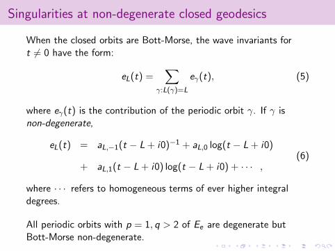
Singularities at non-degenerate closed geodesics

When the closed orbits are Bott-Morse, the wave invariants fort 6= 0 have the form:

eL(t) =∑

γ:L(γ)=L

eγ(t), (5)

where eγ(t) is the contribution of the periodic orbit γ. If γ isnon-degenerate,

eL(t) = aL,−1(t − L + i0)−1 + aL,0 log(t − L + i0)

+ aL,1(t − L + i0) log(t − L + i0) + · · · ,(6)

where · · · refers to homogeneous terms of ever higher integraldegrees.

All periodic orbits with p = 1, q > 2 of Ee are degenerate butBott-Morse non-degenerate.

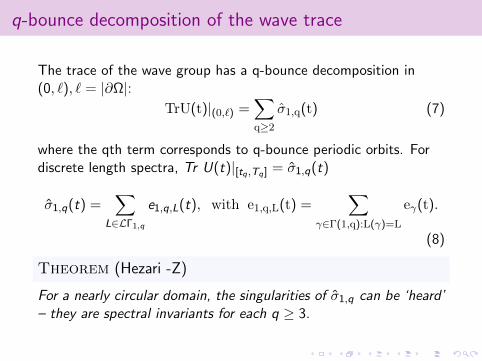
q-bounce decomposition of the wave trace

The trace of the wave group has a q-bounce decomposition in(0, `), ` = |∂Ω|:

TrU(t)|(0,`) =∑

q≥2

σ1,q(t) (7)

where the qth term corresponds to q-bounce periodic orbits. Fordiscrete length spectra, Tr U(t)|[tq ,Tq ] = σ1,q(t)

σ1,q(t) =∑

L∈LΓ1,q

e1,q,L(t), with e1,q,L(t) =∑

γ∈Γ(1,q):L(γ)=L

eγ(t).

(8)

Theorem (Hezari -Z)

For a nearly circular domain, the singularities of σ1,q can be ‘heard’– they are spectral invariants for each q ≥ 3.

Melrose-Marvizi parametrix

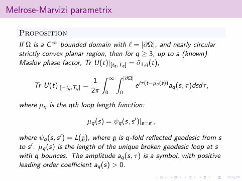
Proposition

If Ω is a C∞ bounded domain with ` = |∂Ω|, and nearly circularstrictly convex planar region, then for q ≥ 3, up to a (known)Maslov phase factor, Tr U(t)|[tq ,Tq ] = σ1,q(t),

Tr U(t)|[−tq ,Tq ] =1

2π

∫ ∞

0

∫ |∂Ω|

0e iτ(t−µq(s))aq(s, τ)dsdτ,

where µq is the qth loop length function:

µq(s) = ψq(s, s ′)|s=s′ ,

where ψq(s, s ′) = L(g), where g is q-fold reflected geodesic from sto s ′. µq(s) is the length of the unique broken geodesic loop at swith q bounces. The amplitude aq(s, τ) is a symbol, with positiveleading order coefficient aq(s) > 0.

Length spectrum multiplicity and audibility

The perennial problem in inverse spectral theory is multiplicity inthe length spectrum – the possibility that the ‘wave tracesingularity invariants’ at two closed geodesics of the same lengthmay cancel each other and be ‘inaudible.’

I Cancellation can only occur for non-degenerate orbits (due toSoga for 1D oscillatory integrals, e.g. the Marvizi-Melroseintegrals);

I Cancellation can only occur if the Maslov indices σ in thephases iσ of two orbits have opposite signs. But all Γ(1, q)orbits with q ≥ 3 and lengths L < |∂Ω| cannot have oppositesign Maslov indices.

Completion of proof

Since one can ‘hear’ σ1,q, for q ≥ 3,

σΩ1,q(t) = σEe

1,q(t),

Proposition

Assume that Ω is isospectral to an ellipse Ee of small eccentricity.Let ` = |∂Ω| = |∂Ee |. Let LEe

q be the loop length function for Ee

(a constant). Then,

∫ `

0e iλµq(s)aq(s, λ)ds = e iλL

Eq

∫ `

0aEeq (s, λ)ds + O(λ−∞).

For an ellipse the right side is a symbol of order 0.

We now show that this equality forces µq(s) to be constant.

µq(s) must be constant

Critical points of µq(s) are points s ∈ ∂Ω where there exists aclosed orbit of the Billiard flow in the class Γ(1, q) starting at s. Inthe case of the ellipse, the loop length function is a constant.The final point is to prove:

Lemma

µq has exactly one critical value. Hence, µq is constant. Thus,every loop is a closed billiard trajectory and a loop exists at everys ∈ ∂Ω.

NOTE: the loop length function µq(s) is one of the main objectswe study. Its variation is the ‘Melnikov function’, the key thingstudied by Avila-de Simoi-Kaloshin.

Final remarks

I Until the last step, where we use that the ‘bands’ collapse topoints, the results hold for all nearly circular domains. Inparticular, the Melrose-Marvizi integrals are spectral invariantsof nearly circular domains. The goal is to ‘recover’ the phaseof the integrals from the asymptotics.

I All periodic orbits of Ee are degenerate except the bouncingball orbits of the major/minor axes. The same would be truefor any isospectral domain if one can rule out cancellations ofwave invariants.

I The critical point set of the phase µq of a general C∞ (even,nearly circular) domain can be an arbitrary closed set, e.g. aCantor set. But for real analytic domains, either the phase isconstant or it has only finitely many isolated critical pointswith finite vanishing order. We can show that it must berationally integrable ‘close to the boundary.’

The four levels of spectral determinacy

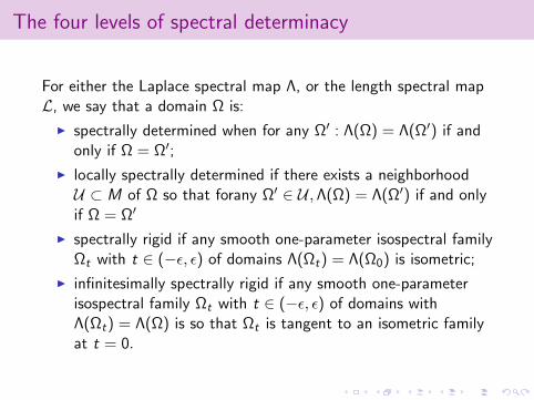
For either the Laplace spectral map Λ, or the length spectral mapL, we say that a domain Ω is:

I spectrally determined when for any Ω′ : Λ(Ω) = Λ(Ω′) if andonly if Ω = Ω′;

I locally spectrally determined if there exists a neighborhoodU ⊂ M of Ω so that forany Ω′ ∈ U ,Λ(Ω) = Λ(Ω′) if and onlyif Ω = Ω′

I spectrally rigid if any smooth one-parameter isospectral familyΩt with t ∈ (−ε, ε) of domains Λ(Ωt) = Λ(Ω0) is isometric;

I infinitesimally spectrally rigid if any smooth one-parameterisospectral family Ωt with t ∈ (−ε, ε) of domains withΛ(Ωt) = Λ(Ω) is so that Ωt is tangent to an isometric familyat t = 0.