Pitfalls in likelihood land

Andrew Fowlie (speaker) & Anders Kvellestad

18 February 2021

Nanjing Normal University

Likelihood land

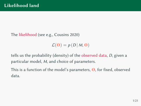
The likelihood (see e.g., Cousins 2020)

L(Θ) = p (D |M,Θ)

tells us the probability (density) of the observed data, D, given a

particular model, M, and choice of parameters.

This is a function of the model’s parameters, Θ, for fixed, observed

data.

1/21

Likelihood land

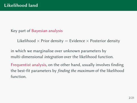
Key part of Bayesian analysis

Likelihood× Prior density = Evidence× Posterior density

in which we marginalise over unknown parameters by

multi-dimensional integration over the likelihood function.

Frequentist analysis, on the other hand, usually involves finding

the best-fit parameters by finding the maximum of the likelihood

function.

2/21

General pitfalls

Pitfall — the likelihood is not enough?

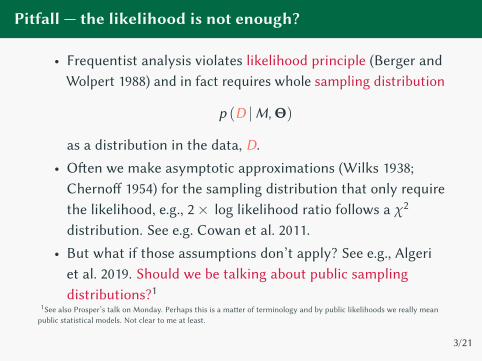
• Frequentist analysis violates likelihood principle (Berger and

Wolpert 1988) and in fact requires whole sampling distribution

p (D |M,Θ)

as a distribution in the data, D.

• O�en we make asymptotic approximations (Wilks 1938;

Cherno� 1954) for the sampling distribution that only require

the likelihood, e.g., 2× log likelihood ratio follows a χ2

distribution. See e.g. Cowan et al. 2011.

• But what if those assumptions don’t apply? See e.g., Algeri

et al. 2019. Should we be talking about public sampling

distributions?1

1See also Prosper’s talk on Monday. Perhaps this is a ma�er of terminology and by public likelihoods we really mean

public statistical models. Not clear to me at least.

3/21

Common pitfalls

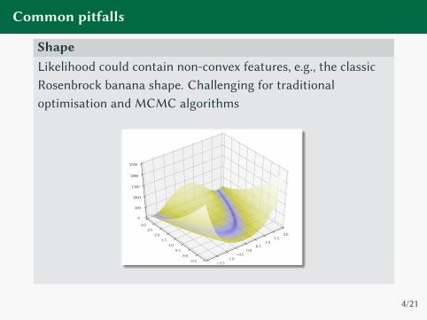
ShapeLikelihood could contain non-convex features, e.g., the classic

Rosenbrock banana shape. Challenging for traditional

optimisation and MCMC algorithms

−2.0−1.5

−1.0−0.5

0.00.5

1.01.5

2.0

−1.0

−0.5

0.0

0.5

1.0

1.5

2.0

2.5

3.0

0

500

1000

1500

2000

2500

4/21

Common pitfalls

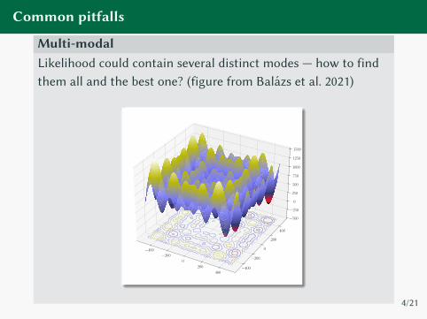
Multi-modalLikelihood could contain several distinct modes — how to find

them all and the best one? (figure from Balazs et al. 2021)

−400

−200

0

200

400−400

−200

0

200

400

−500

−250

0

250

500

750

1000

1250

1500

4/21

Common pitfalls

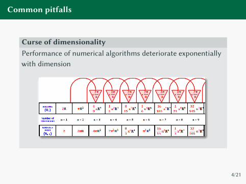
Curse of dimensionalityPerformance of numerical algorithms deteriorate exponentially

with dimension

4/21

Common pitfalls

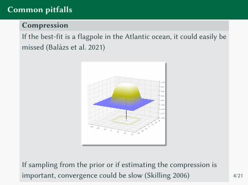
CompressionIf the best-fit is a flagpole in the Atlantic ocean, it could easily be

missed (Balazs et al. 2021)

−30 −20 −100

1020

30−30−20−10

010

2030

−1.00

−0.75

−0.50

−0.25

0.00

0.25

0.50

0.75

1.00

If sampling from the prior or if estimating the compression is

important, convergence could be slow (Skilling 2006) 4/21

Common pitfalls

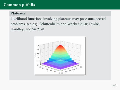
PlateausLikelihood functions involving plateaus may pose unexpected

problems, see e.g., Schi�enhelm and Wacker 2020; Fowlie,

Handley, and Su 2020

x

0.00.2

0.40.6

0.81.0

y

0.00.2

0.40.6

0.81.0

L(x,

y)

0.0

0.2

0.4

0.6

0.8

1.0

4/21

Pitfall — incomplete information

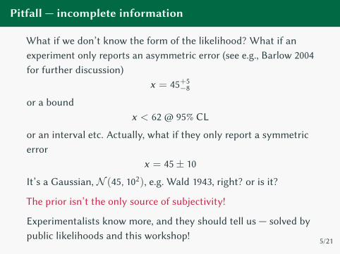
What if we don’t know the form of the likelihood? What if an

experiment only reports an asymmetric error (see e.g., Barlow 2004

for further discussion)

x = 45+5

−8

or a bound

x < 62 @ 95% CL

or an interval etc. Actually, what if they only report a symmetric

error

x = 45± 10

It’s a Gaussian, N (45, 102), e.g. Wald 1943, right? or is it?

The prior isn’t the only source of subjectivity!

Experimentalists know more, and they should tell us — solved by

public likelihoods and this workshop!5/21

Pitfall — intractable likelihood

What if we just can’t work out the likelihood — it’s intractable?

Fine — if we can draw pseudo data from the sampling distribution

we can use likelihood-free inference methods, e.g., ABC (Diggle

and Gra�on 1984).

Public sampling distributions?

6/21

Pitfall — noisy estimate of likelihood

Consider case of LHC likelihoods. The likelihood might be a

Poisson involving the expected number of events.

The expected number of events, though, can o�en only be

computed through forward simulations of the whole experiment,

involving MC simulations in e.g., Pythia and detector simulations

So we end up with a noisy estimate of the likelihood, L.

7/21

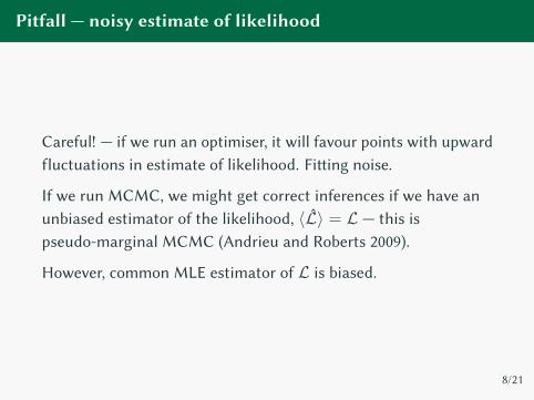
Pitfall — noisy estimate of likelihood

Careful! — if we run an optimiser, it will favour points with upward

fluctuations in estimate of likelihood. Fi�ing noise.

If we run MCMC, we might get correct inferences if we have an

unbiased estimator of the likelihood, 〈L〉 = L — this is

pseudo-marginal MCMC (Andrieu and Roberts 2009).

However, common MLE estimator of L is biased.

8/21

Interplay between noise and incompleteinformation

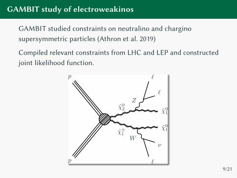
GAMBIT study of electroweakinos

GAMBIT studied constraints on neutralino and chargino

supersymmetric particles (Athron et al. 2019)

Compiled relevant constraints from LHC and LEP and constructed

joint likelihood function.

χ±1

χ02

W

Z

p

p

`

ν

χ01

χ01

`

`

9/21

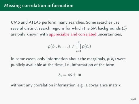
Missing correlation information

CMS and ATLAS perform many searches. Some searches use

several distinct search regions for which the SM backgrounds (b)

are only known with appreciable and correlated uncertainties,

p(b1, b2, . . .) 6=n

∏i=1

p(bi)

In some cases, only information about the marginals, p(bi) were

publicly available at the time, i.e., information of the form

b1 = 46± 10

without any correlation information, e.g., a covariance matrix.

10/21

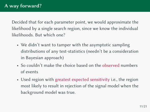
A way forward?

Decided that for each parameter point, we would approximate the

likelihood by a single search region, since we know the individual

likelihoods. But which one?

• We didn’t want to tamper with the asymptotic sampling

distributions of any test-statistics (needn’t be a consideration

in Bayesian approach)

• So couldn’t make the choice based on the observed numbers

of events

• Used region with greatest expected sensitivity i.e., the region

most likely to result in rejection of the signal model when the

background model was true.

11/21

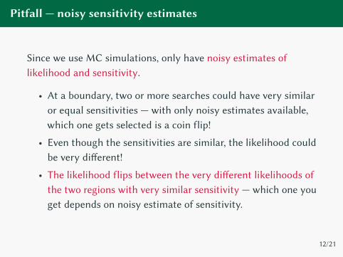
Pitfall — noisy sensitivity estimates

Since we use MC simulations, only have noisy estimates of

likelihood and sensitivity.

• At a boundary, two or more searches could have very similar

or equal sensitivities — with only noisy estimates available,

which one gets selected is a coin flip!

• Even though the sensitivities are similar, the likelihood could

be very di�erent!

• The likelihood flips between the very di�erent likelihoods of

the two regions with very similar sensitivity — which one you

get depends on noisy estimate of sensitivity.

12/21

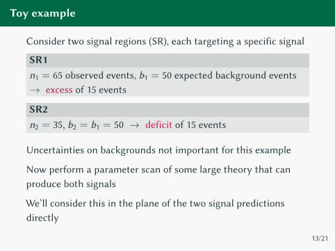
Toy example

Consider two signal regions (SR), each targeting a specific signal

SR1n1 = 65 observed events, b1 = 50 expected background events

→ excess of 15 events

SR2n2 = 35, b2 = b1 = 50 → deficit of 15 events

Uncertainties on backgrounds not important for this example

Now perform a parameter scan of some large theory that can

produce both signals

We’ll consider this in the plane of the two signal predictions

directly

13/21

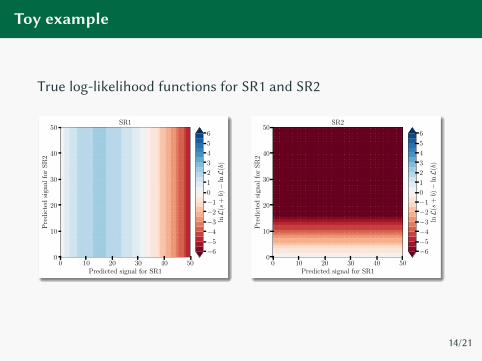
Toy example

True log-likelihood functions for SR1 and SR2

0 10 20 30 40 50Predicted signal for SR1

0

10

20

30

40

50

Pre

dic

ted

sign

alfo

rS

R2

SR1

−6

−5

−4

−3

−2

−1

0

1

2

3

4

5

6

lnL(s

+b)−

lnL(b)

0 10 20 30 40 50Predicted signal for SR1

0

10

20

30

40

50

Pre

dic

ted

sign

alfo

rS

R2

SR2

−6

−5

−4

−3

−2

−1

0

1

2

3

4

5

6

lnL(s

+b)−

lnL(b)

14/21

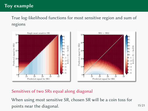
Toy example

True log-likelihood functions for most sensitive region and sum of

regions

0 10 20 30 40 50Predicted signal for SR1

0

10

20

30

40

50

Pre

dic

ted

sign

alfo

rS

R2

Single most sensitive SR

−6

−5

−4

−3

−2

−1

0

1

2

3

4

5

6

lnL(s

+b)−

lnL(b)

0 10 20 30 40 50Predicted signal for SR1

0

10

20

30

40

50

Pre

dic

ted

sign

alfo

rS

R2

SR1 + SR2

−6

−5

−4

−3

−2

−1

0

1

2

3

4

5

6

lnL(s

+b)−

lnL(b)

Sensitives of two SRs equal along diagonal

When using most sensitive SR, chosen SR will be a coin toss for

points near the diagonal.15/21

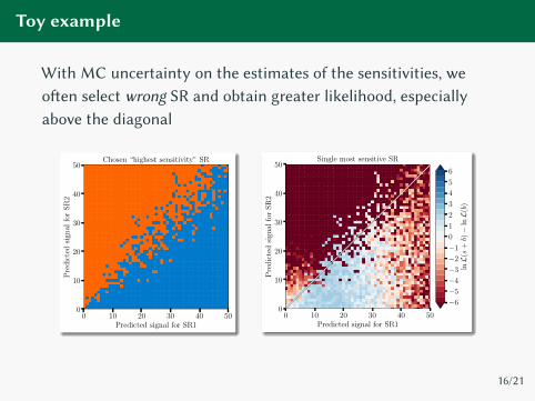
Toy example

With MC uncertainty on the estimates of the sensitivities, we

o�en select wrong SR and obtain greater likelihood, especially

above the diagonal

0 10 20 30 40 50Predicted signal for SR1

0

10

20

30

40

50

Pre

dic

ted

sign

alfo

rS

R2

Chosen “highest sensitivity” SR

0 10 20 30 40 50Predicted signal for SR1

0

10

20

30

40

50

Pre

dic

ted

sign

alfo

rS

R2

Single most sensitive SR

−6

−5

−4

−3

−2

−1

0

1

2

3

4

5

6

lnL(s

+b)−

lnL(b)

16/21

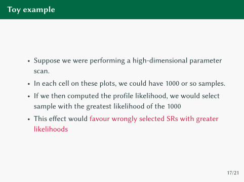
Toy example

• Suppose we were performing a high-dimensional parameter

scan.

• In each cell on these plots, we could have 1000 or so samples.

• If we then computed the profile likelihood, we would select

sample with the greatest likelihood of the 1000

• This e�ect would favour wrongly selected SRs with greater

likelihoods

17/21

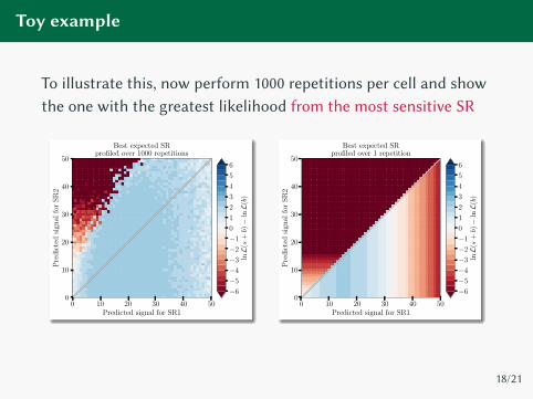
Toy example

To illustrate this, now perform 1000 repetitions per cell and show

the one with the greatest likelihood from the most sensitive SR

0 10 20 30 40 50Predicted signal for SR1

0

10

20

30

40

50

Pre

dic

ted

sign

alfo

rS

R2

Best expected SRprofiled over 1000 repetitions

−6

−5

−4

−3

−2

−1

0

1

2

3

4

5

6

lnL(s

+b)−

lnL(b)

0 10 20 30 40 50Predicted signal for SR1

0

10

20

30

40

50

Pre

dic

ted

sign

alfo

rS

R2

Best expected SRprofiled over 1 repetition

−6

−5

−4

−3

−2

−1

0

1

2

3

4

5

6

lnL(s

+b)−

lnL(b)

18/21

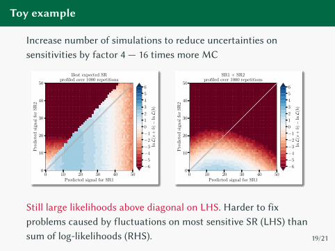
Toy example

Increase number of simulations to reduce uncertainties on

sensitivities by factor 4 — 16 times more MC

0 10 20 30 40 50Predicted signal for SR1

0

10

20

30

40

50

Pre

dic

ted

sign

alfo

rS

R2

Best expected SRprofiled over 1000 repetitions

−6

−5

−4

−3

−2

−1

0

1

2

3

4

5

6

lnL(s

+b)−

lnL(b)

0 10 20 30 40 50Predicted signal for SR1

0

10

20

30

40

50

Pre

dic

ted

sign

alfo

rS

R2

SR1 + SR2profiled over 1000 repetitions

−6

−5

−4

−3

−2

−1

0

1

2

3

4

5

6

lnL(s

+b)−

lnL(b)

Still large likelihoods above diagonal on LHS. Harder to fix

problems caused by fluctuations on most sensitive SR (LHS) than

sum of log-likelihoods (RHS). 19/21

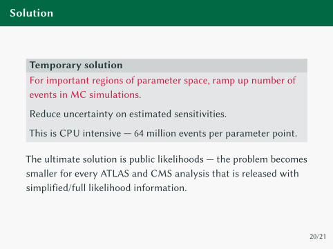
Solution

Temporary solutionFor important regions of parameter space, ramp up number of

events in MC simulations.

Reduce uncertainty on estimated sensitivities.

This is CPU intensive — 64 million events per parameter point.

The ultimate solution is public likelihoods — the problem becomes

smaller for every ATLAS and CMS analysis that is released with

simplified/full likelihood information.

20/21

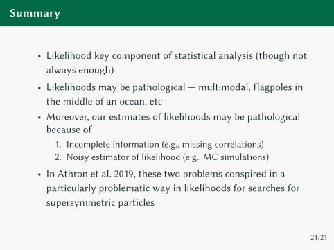
Summary

• Likelihood key component of statistical analysis (though not

always enough)

• Likelihoods may be pathological — multimodal, flagpoles in

the middle of an ocean, etc

• Moreover, our estimates of likelihoods may be pathological

because of

1. Incomplete information (e.g., missing correlations)

2. Noisy estimator of likelihood (e.g., MC simulations)

• In Athron et al. 2019, these two problems conspired in a

particularly problematic way in likelihoods for searches for

supersymmetric particles

21/21

Backup

Bayesian land

Here, we don’t care about spoiling or knowing sampling behaviour.

We can just build the best approximation to the likelihood. This

problem needn’t occur.

Possible approaches:

• We know the marginals. We want write the joint distribution.

A general approach is this problem is that of copulas (Nelsen

2006). Schematically,

every joint distribution = marginal distributions + copula

• Make approximation of likelihood using observed counts, e.g.,

crude bound

L ≤ mini

P (searchi |M,Θ)

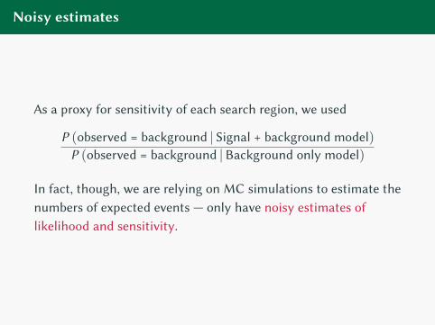
Noisy estimates

As a proxy for sensitivity of each search region, we used

P (observed = background | Signal + background model)

P (observed = background |Background only model)

In fact, though, we are relying on MC simulations to estimate the

numbers of expected events — only have noisy estimates of

likelihood and sensitivity.

References i

References

Algeri, Sara et al. (Nov. 2019). “Searching for new physics with

profile likelihoods: Wilks and beyond.” In: arXiv: 1911.10237

[physics.data-an].

Andrieu, Christophe and Gareth O. Roberts (Apr. 2009). “The

pseudo-marginal approach for e�icient Monte Carlo

computations.” In: Ann. Statist. 37.2, pp. 697–725. url:

h�ps://doi.org/10.1214/07-AOS574.

Athron, Peter et al. (2019). “Combined collider constraints on

neutralinos and charginos.” In: Eur. Phys. J. C 79.5, p. 395. arXiv:

1809.02097 [hep-ph].

References ii

Balazs, Csaba et al. (Jan. 2021). “A comparison of optimisation

algorithms for high-dimensional particle and astrophysics

applications.” In: arXiv: 2101.04525 [hep-ph].

Barlow, Roger (June 2004). “Asymmetric statistical errors.” In:

Statistical Problems in Particle Physics, Astrophysics andCosmology, pp. 56–59. arXiv: physics/0406120.

Berger, J.O. and R.L. Wolpert (1988). The Likelihood Principle.Institute of Mathematical Statistics. Lecture notes : monographs

series. Institute of Mathematical Statistics. isbn: 9780940600133.

Cherno�, Herman (Sept. 1954). “On the Distribution of the

Likelihood Ratio.” In: Ann. Math. Statist. 25.3, pp. 573–578. url:

h�ps://doi.org/10.1214/aoms/1177728725.

References iii

Cousins, Robert D. (Oct. 2020). “What is the likelihood function,

and how is it used in particle physics?” In: arXiv: 2010.00356

[physics.data-an].

Cowan, Glen et al. (2011). “Asymptotic formulae for

likelihood-based tests of new physics.” In: Eur. Phys. J. C 71.

[Erratum: Eur.Phys.J.C 73, 2501 (2013)], p. 1554. arXiv: 1007.1727

[physics.data-an].

Diggle, Peter J. and Richard J. Gra�on (1984). “Monte Carlo

Methods of Inference for Implicit Statistical Models.” In: Journalof the Royal Statistical Society. Series B (Methodological) 46.2,

pp. 193–227. issn: 00359246. url:

h�p://www.jstor.org/stable/2345504.

References iv

Fowlie, Andrew, Will Handley, and Liangliang Su (Oct. 2020).

“Nested sampling with plateaus.” In: arXiv: 2010.13884

[stat.CO].

Nelsen, R.B. (2006). An Introduction to Copulas. Springer Series in

Statistics. Springer. isbn: 9780387286594. url:

h�ps://books.google.com/books?id=B3ONT5rBv0wC.

Schi�enhelm, Doris and Philipp Wacker (May 2020). “Nested

Sampling And Likelihood Plateaus.” In: arXiv e-prints,arXiv:2005.08602, arXiv:2005.08602. arXiv: 2005.08602 [math.ST].

Skilling, John (Dec. 2006). “Nested sampling for general Bayesian

computation.” In: Bayesian Anal. 1.4, pp. 833–859. url:

h�ps://doi.org/10.1214/06-BA127.

References v

Wald, Abraham (1943). “Tests of Statistical Hypotheses Concerning

Several Parameters When the Number of Observations is Large.”

In: Transactions of the American Mathematical Society 54.3,

pp. 426–482. issn: 00029947. url:

h�p://www.jstor.org/stable/1990256.

Wilks, S. S. (1938). “The Large-Sample Distribution of the

Likelihood Ratio for Testing Composite Hypotheses.” In: AnnalsMath. Statist. 9.1, pp. 60–62.