18.650 (F16) Lecture 3: Maximum Likelihood Estimation
25
18.650 Statistics for Applications Chapter 3: Maximum Likelihood Estimation 1/23
Transcript of 18.650 (F16) Lecture 3: Maximum Likelihood Estimation
18.650
Statistics for Applications
Chapter 3: Maximum Likelihood Estimation
1/23
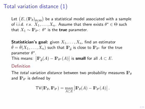
Total variation distance (1)
Let (E, (IPθ)θ∈Θ
) be a statistical model associated with a sample
of i.i.d. r.v. X1, . . . ,Xn. Assume that there exists θ∗ ∈ Θ such that X1 ∼ IPθ∗ : θ
∗ is the true parameter.
Statistician’s goal: given X1, . . . ,Xn, find an estimator ˆ ˆθ = θ(X1, . . . ,Xn) such that IPˆ is close to IPθ∗ for the true θ
parameter θ∗ . This means:
IPˆ(A)− IPθ∗ (A)
is small for all A ⊂ E. θ
Definition
The total variation distance between two probability measures IPθ
and IPθ′ is defined by
TV(IPθ, IPθ′ ) = max IPθ(A)− IPθ′ (A)
. A⊂E
2/23
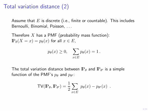
Total variation distance (2)
Assume that E is discrete (i.e., finite or countable). This includes Bernoulli, Binomial, Poisson, . . .
Therefore X has a PMF (probability mass function): IPθ(X = x) = pθ(x) for all x ∈ E,
Lpθ(x) ≥ 0, pθ(x) = 1 .
x∈E
The total variation distance between IPθ and IPθ′ is a simple function of the PMF’s pθ and pθ′ :
1 LTV(IPθ, IPθ′ ) = pθ(x)− pθ′ (x) .
2 x∈E
3/23
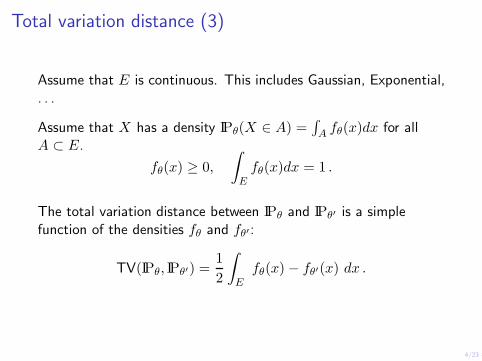
Total variation distance (3)
Assume that E is continuous. This includes Gaussian, Exponential, . . .
Assume that X has a density IPθ(X ∈ A) = J
fθ(x)dx for all A
A ⊂ E. lfθ(x) ≥ 0, fθ(x)dx = 1 .
E
The total variation distance between IPθ and IPθ′ is a simple function of the densities fθ and fθ′ :
1 l
TV(IPθ, IPθ′ ) = fθ(x)− fθ′ (x) dx . 2 E
4/23
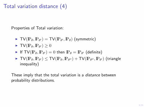
Total variation distance (4)
Properties of Total variation:
◮ TV(IPθ, IPθ′ ) = TV(IPθ′ , IPθ) (symmetric)
◮ TV(IPθ, IPθ′ ) ≥ 0 ◮ If TV(IPθ, IPθ′ ) = 0 then IPθ = IPθ′ (definite)
◮ TV(IPθ, IPθ′ ) ≤ TV(IPθ, IPθ′′ ) + TV(IPθ′′ , IPθ′ ) (triangle inequality)
These imply that the total variation is a distance between probability distributions.
5/23
Total variation distance (5)
An estimation strategy: Build an estimator T for all TV(IPθ, IPθ∗ )
θ ∈ Θ. Then find ˆ TV(IPθ, IPθ∗ ).θ that minimizes the function θ → T
6/23
Total variation distance (5)
An estimation strategy: Build an estimator T for all TV(IPθ, IPθ∗ )
θ ∈ Θ. Then find ˆ TV(IPθ, IPθ∗ ).θ that minimizes the function θ → T
problem: Unclear how to build TTV(IPθ, IPθ∗ )!
6/23
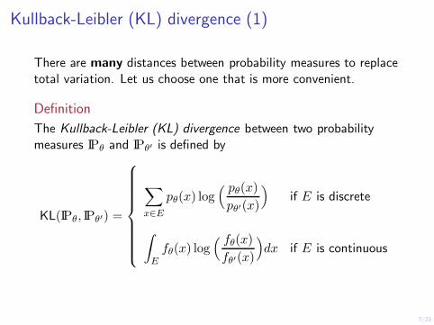
Kullback-Leibler (KL) divergence (1)
There are many distances between probability measures to replace total variation. Let us choose one that is more convenient.
Definition
The Kullback-Leibler (KL) divergence between two probability measures IPθ and IPθ′ is defined by
KL(IPθ, IPθ′ ) =
L
x∈E
pθ(x) log( pθ(x) pθ′ (x)
) if E is discrete
l
E
fθ(x) log( fθ(x) fθ′ (x)
)dx if E is continuous
7/23
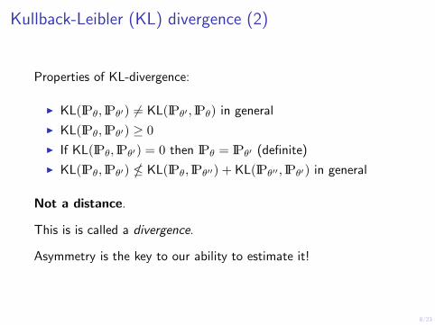
Kullback-Leibler (KL) divergence (2)
Properties of KL-divergence:
◮ KL(IPθ, IPθ′ ) = KL(IPθ′ , IPθ) in general
◮ KL(IPθ, IPθ′ ) ≥ 0 ◮ If KL(IPθ, IPθ′ ) = 0 then IPθ = IPθ′ (definite)
◮ KL(IPθ, IPθ′ ) i KL(IPθ, IPθ′′ ) + KL(IPθ′′ , IPθ′ ) in general
Not a distance.
This is is called a divergence.
Asymmetry is the key to our ability to estimate it!
8/23
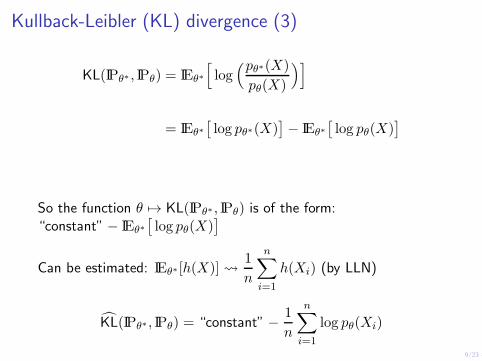
Kullback-Leibler (KL) divergence (3)
KL(IPθ∗ , IPθ) = IEθ∗
[ log(pθ∗ (X))] pθ(X)
= IEθ∗ [ log pθ∗ (X)
] − IEθ∗
[ log pθ(X)
]
So the function θ → KL(IPθ∗ , IPθ) is of the form: “constant” − IEθ∗
[ log pθ(X)
]
n1
Can be estimated: IEθ∗ [h(X)] -L
h(Xi) (by LLN) n
i=1
n1
KL(IPθ∗ , IPθ) = “constant” − L
log pθ(Xi)Tn
i=1 9/23
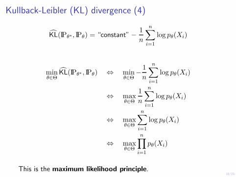
Kullback-Leibler (KL) divergence (4)
KL(IPθ∗ , IPθ)
KL(IPθ∗ , IPθ)T
Tn
n i=1
L1 “constant” − log pθ(Xi)=
n
θ∈Θ n i=1
L1 min ⇔ min − log pθ(Xi) θ∈Θ
nL1 ⇔ max
Ln⇔ max
log pθ(Xi) θ∈Θ n
i=1
log pθ(Xi) θ∈Θ
i=1 n
pθ(Xi)n
⇔ max i=1
This is the maximum likelihood principle.
θ∈Θ
10/23
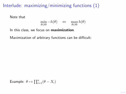
Interlude: maximizing/minimizing functions (1)
Note that min −h(θ) ⇔ max h(θ) θ∈Θ θ∈Θ
In this class, we focus on maximization.
Maximization of arbitrary functions can be difficult:
Example: θ → �n (θ −Xi)i=1
11/23
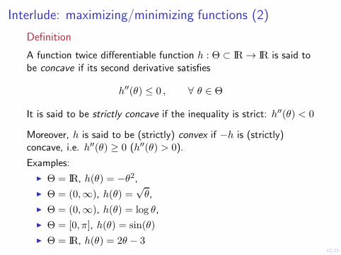
Interlude: maximizing/minimizing functions (2)
Definition
A function twice differentiable function h : Θ ⊂ IR → IR is said to be concave if its second derivative satisfies
h ′′ (θ) ≤ 0 , ∀ θ ∈ Θ
It is said to be strictly concave if the inequality is strict: h ′′ (θ) < 0
Moreover, h is said to be (strictly) convex if −h is (strictly) concave, i.e. h ′′ (θ) ≥ 0 (h ′′ (θ) > 0).
Examples:
◮ Θ = IR, h(θ) = −θ2 ,√ ◮ Θ = (0,∞), h(θ) = θ,
◮ Θ = (0,∞), h(θ) = log θ,
◮ Θ = [0, π], h(θ) = sin(θ)
◮ Θ = IR, h(θ) = 2θ − 3 12/23
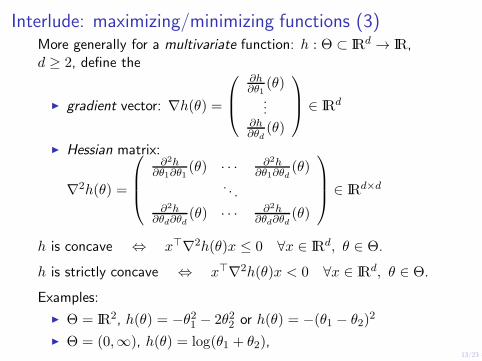
Interlude: maximizing/minimizing functions (3) More generally for a multivariate function: h : Θ ⊂ IRd → IR, d ≥ 2, define the
∈ IRd
◮ gradient vector: ∇h(θ) =
∂h ∂θ1
(θ) . . .
∂h ∂θd
(θ)
◮ Hessian matrix: ∂2h ∂2h(θ) · · · (θ)
∂θ1∂θ1 ∂θ1∂θd
∇2h(θ) =
. ∈ IRd×d. .
∂2h ∂2h(θ) · · · (θ)∂θd∂θd ∂θd∂θd
h is concave ⇔ x⊤∇2h(θ)x ≤ 0 ∀x ∈ IRd, θ ∈ Θ.
h is strictly concave ⇔ x⊤∇2h(θ)x < 0 ∀x ∈ IRd, θ ∈ Θ.
Examples:
◮ Θ = IR2 , h(θ) = −θ12 − 2θ2
2 or h(θ) = −(θ1 − θ2)2
◮ Θ = (0,∞), h(θ) = log(θ1 + θ2), 13/23
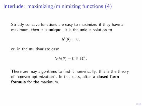
Interlude: maximizing/minimizing functions (4)
Strictly concave functions are easy to maximize: if they have a maximum, then it is unique. It is the unique solution to
h ′ (θ) = 0 ,
or, in the multivariate case
∇h(θ) = 0 ∈ IRd .
There are may algorithms to find it numerically: this is the theory of “convex optimization”. In this class, often a closed form formula for the maximum.
14/23
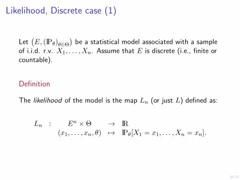
Likelihood, Discrete case (1)
Let (E, (IPθ)θ∈Θ
) be a statistical model associated with a sample
of i.i.d. r.v. X1, . . . ,Xn. Assume that E is discrete (i.e., finite or countable).
Definition
The likelihood of the model is the map Ln (or just L) defined as:
Ln : En ×Θ → IR (x1, . . . , xn, θ) → IPθ[X1 = x1, . . . ,Xn = xn].
15/23
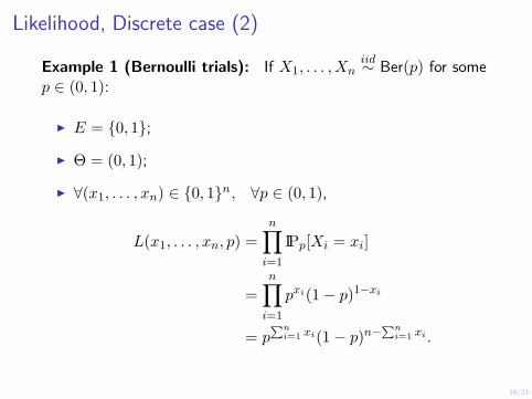
Likelihood, Discrete case (2)
iidExample 1 (Bernoulli trials): If X1, . . . ,Xn ∼ Ber(p) for some p ∈ (0, 1):
◮ E = {0, 1}; ◮ Θ = (0, 1);
◮ ∀(x1, . . . , xn) ∈ {0, 1}n , ∀p ∈ (0, 1), n
L(x1, . . . , xn, p) = n
IPp[Xi = xi] i=1 n
= n
p xi (1− p)1−xi
i=1
xii=1 i=1 = p�
n xi (1− p)n−�
n .
16/23
�
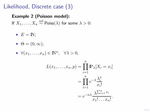
Likelihood, Discrete case (3)
Example 2 (Poisson model): iid
If X1, . . . ,Xn ∼ Poiss(λ) for some λ > 0:
◮ E = IN;
◮ Θ = (0,∞);
◮ ∀(x1, . . . , xn) ∈ INn , ∀λ > 0,
n
L(x1, . . . , xn, p) = n
IPλ[Xi = xi] i=1 n
−λ λx i =
n e
xi! i=1
n λ i=1 xi
−nλ = e . x1! . . . xn!
17/23
�
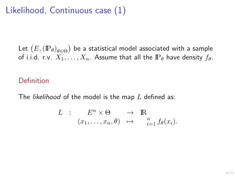
Likelihood, Continuous case (1)
Let (E, (IPθ)θ∈Θ
) be a statistical model associated with a sample
of i.i.d. r.v. X1, . . . ,Xn. Assume that all the IPθ have density fθ.
Definition
The likelihood of the model is the map L defined as:
L : En ×Θ → IR n(x1, . . . , xn, θ) → fθ(xi).i=1
18/23
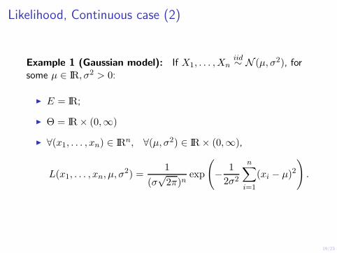
Likelihood, Continuous case (2)
iidExample 1 (Gaussian model): If X1, . . . ,Xn ∼ N (µ, σ2), for some µ ∈ IR, σ2 > 0:
◮ E = IR;
◮ Θ = IR× (0,∞)
◮ ∀(x1, . . . , xn) ∈ IRn , ∀(µ, σ2) ∈ IR× (0,∞),
n
1 1 L(x1, . . . , xn, µ, σ
2) = √ exp − L
(xi − µ)2 . 2π)n 2σ2(σ
i=1
19/23
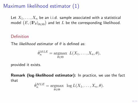
Maximum likelihood estimator (1)
Let X1, . . . ,Xn be an i.i.d. sample associated with a statistical model
(E, (IPθ)θ∈Θ
) and let L be the corresponding likelihood.
Definition
The likelihood estimator of θ is defined as:
θMLE = argmax L(X1, . . . ,Xn, θ),n θ∈Θ
provided it exists.
Remark (log-likelihood estimator): In practice, we use the fact that
θMLE = argmax logL(X1, . . . ,Xn, θ).n θ∈Θ
20/23
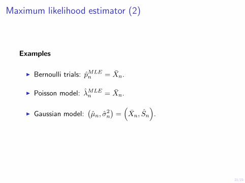
Maximum likelihood estimator (2)
Examples
¯◮ Bernoulli trials: pMLE = Xn.n
λMLE ¯◮ Poisson model: ˆ = Xn.n
◮ Gaussian model: (µn, σ
2) = (Xn, Sn
).n
21/23
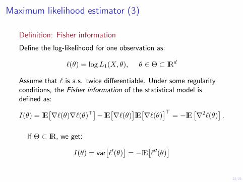
Maximum likelihood estimator (3)
Definition: Fisher information
Define the log-likelihood for one observation as:
ℓ(θ) = logL1(X, θ), θ ∈ Θ ⊂ IRd
Assume that ℓ is a.s. twice differentiable. Under some regularity conditions, the Fisher information of the statistical model is defined as:
I(θ) = IE[∇ℓ(θ)∇ℓ(θ)⊤
] − IE
[∇ℓ(θ)
]IE[∇ℓ(θ)
]⊤ = −IE
[∇2ℓ(θ)
] .
If Θ ⊂ IR, we get:
I(θ) = var[ℓ ′ (θ)
] = −IE
[ℓ ′′ (θ)
]
22/23
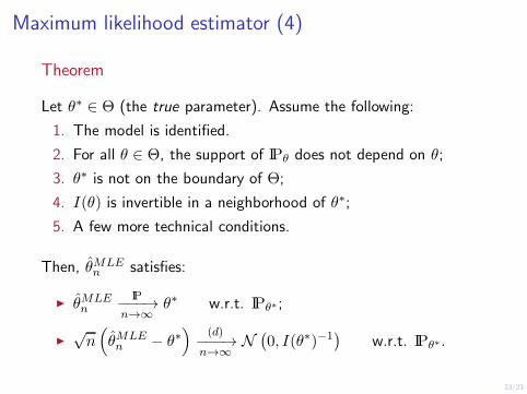
Maximum likelihood estimator (4)
Theorem
Let θ∗ ∈ Θ (the true parameter). Assume the following:
1. The model is identified.
2. For all θ ∈ Θ, the support of IPθ does not depend on θ;
3. θ∗ is not on the boundary of Θ;
4. I(θ) is invertible in a neighborhood of θ∗ ;
5. A few more technical conditions.
θMLE Then, ˆ satisfies: n
θMLE IP◮ ˆ −−−→ θ ∗ w.r.t. IPθ∗ ;n
n→∞
√ (d)◮ n
(θMLE − θ ∗
) −−−→ N
(0, I(θ ∗ )−1
) w.r.t. IPθ∗ .n
n→∞
23/23

MIT OpenCourseWare https://ocw.mit.edu
18.650 / 18.6501 Statistics for Applications Fall 2016
For information about citing these materials or our Terms of Use, visit: https://ocw.mit.edu/terms.