Automated Simplification of Large Symbolic

Expressions

David H. Bailey

Lawrence Berkeley National Laboratory,Berkeley, CA 94720

Jonathan M. Borwein

Centre for Computer Assisted Research Mathematics and its Applications (CARMA),Laureate Professor, Univ of Newcastle, Callaghan, NSW 2308, Australia

Alexander D. Kaiser

Courant Institute of Mathematical Sciences, New York University,New York, NY 10012

Abstract

We present a set of algorithms for automated simplification of symbolic constants of the formPi αixi with αi rational and xi complex. The included algorithms, called SimplifySum 1 and

implemented in Mathematica, remove redundant terms, attempt to make terms and the fullexpression real, and remove terms using repeated application of the multipair PSLQ integerrelation detection algorithm. Also included are facilities for making substitutions accordingto user-specified identities. We illustrate this toolset by giving some real-world examples of itsusage, including one, for instance, where the tool reduced a symbolic expression of approximately100,000 characters in size enough to enable manual manipulation to one with just four simpleterms.

Key words: Simplification, Computer Algebra Systems, Experimental Mathematics, ErrorCorrection

1 Available from https://github.com/alexkaiser/SimplifySum

Preprint submitted to Elsevier 13 September 2013

1. Introduction

A common occurrence for many researchers who engage in computational mathematicsis that the result of a Computer Algebra System (CAS) operation, in say Mathematicaor Maple, is a very long, complicated expression, which although technically correct, isnot very helpful; only later do these researchers discover, often indirectly, that in factthe complicated expression they produced further simplifies, sometimes dramatically, tosomething much more elegant and useful. With some frequency the CAS will provide noanswer and may well ‘hang’. Such events are to be expected, given the limitations of anysymbolic computing package, for any of a number of reasons, including the difficulty ofrecognizing when a given subexpression is zero.

Such instances are closely related to the problem of recognizing a numerical valueas a closed-form expression. In this case, researchers have used integer relation-findingalgorithms, such as the PSLQ algorithm and its variants (Bailey and Broadhurst, 2000),to express the given numerical value as a linear sum of constants or terms. In both in-stances, researchers seek as simple a closed-form expression as possible. Such simplifiedclosed-form expressions are highly desirable, both in mathematical research and in prob-lems, say, from mathematical physics. The various definitions and importance of closedforms is described in (Borwein and Crandall, 2013; Chow, 1999). Examples of such workare described in (Bailey et al., 2010b) and (Borwein et al., 2010).

We present herein a software package SimplifySum for the simplification of symbolicconstants of the form

∑i αixi, where each αi is rational and each xi real or complex.

Such constants frequently arise in looking for closed forms for integrals or sums, andare frequently large and machine-generated by symbolic mathematics software such asMathematica or Maple.

Implemented in Mathematica, our package includes a focused set of tools for simplifica-tion of such constants. The package is able to remove redundant constants, opposites andconjugates, symbolically, numerically or both. It can simplify complex terms, which isuseful if some xi are complex yet the whole constant is real. The package uses symbolicalgebra to repeatedly apply the multipair variant of the PSLQ integer relation detec-tion algorithm, and reduces expressions using exact, rational number arithmetic. It alsocontains code to apply substitutions, so the user may specify identities or substitutionsthey would like performed. These tools can be accessed through a convenient, simplefunction interface. Users also have access to the individual functions that can thence becustomized.

The criterion to decide which version of an expression is simpler is straightforward —a sum that has fewer terms is simpler. 2 All the algorithms (with the exception of sub-stitution) only process the rational coefficients αi, so an expression

∑mi=1 αixi is simpler

? Supported in part by the Director, Office of Computational and Technology Research, Division ofMathematical, Information, and Computational Sciences of the U.S. Department of Energy, under con-

tract number DE-AC02-05CH11231. (David H. Bailey)

Email addresses: dhbailey@lbl.gov (David H. Bailey), jonathan.borwein@newcastle.edu.au

(Jonathan M. Borwein), adkaiser@gmail.com (Alexander D. Kaiser).

URLs: http://crd.lbl.gov/~dhbailey/ (David H. Bailey), http://carma.newcastle.edu.au/jon/

(Jonathan M. Borwein), http://cims.nyu.edu/~adk354 (Alexander D. Kaiser).2 For short expressions this may occasionally lead to less elegant presentation; for longer ones it seems

highly desirable.

2

than∑ni=1 βixi if m < n. This is in contrast to the general case discussed in (Carette,

2004), where the question of which version of a general expression is considered andformalized. Because of the restriction to sums, our definition is nearly always consistentwith the Carette’s formalism. In general, the package does not alter xi in simplification,it only removes terms and alters the rational coefficients. Unless the new αi are verycomplex, the resulting expression is simpler. Note that if the user requests substitutions(as described in section 3) then the substitution will be made regardless of whether thisreduces or increases the complexity.

The tools have proven quite effective. Many computer-generated constants have in-stances of the simple redundancies described above. The techniques using integer-relationsare general and reliable, provided numerical results are used with appropriate caution.The substitutions allow the user to apply specific identities automatically. This will allowthem to use identities that arise repeatedly in particular work, but are not in Mathemat-ica.

Note also that the restriction to sums is very general — no limit is placed on each xi,only that it must evaluate to a real or complex number, so each xi may be arbitrarilycomplicated. Each term will be treated as a single constant by all parts of the code, withthe exception of substitutions.

The remainder of the paper is structured as follows. In Section 2 existing literatureon simplification and simplification in current CAS is discussed. In Section 3 the generalstructure of SimplifySum is described. Precise descriptions of the package are relegatedto an Appendix (Section 7). In Section 4 we give a variety of illustrative examples, thenconclude in section 5 with timing and results on some large research constants.

All tests were performed on a stock 2012 MacBook Pro with a 2.9 GHz Intel Core i7processor and 8 GB of RAM using Mathematica 7.01.

2. Related Literature and Previous Work

There are two central questions to consider when designing a simplification algorithm.First, what does it mean for an expression to be simpler than another? Second, given aconstant, what algorithms can be applied to make the expression simpler?

2.1. Simplification in the literature

The paper (Carette, 2004) provides a formal description of simplification. The authordiscusses, using ideas including Kolmogorov complexity and minimum description length,a method for defining whether a version of an expression is simpler than another. Theauthor also discusses use of this formalism to make practical decisions on simplificationof particular expressions and discusses the relationship of his formalism and the simpli-fication algorithms included with Maple. Notably, the author also discusses the lack ofavailable literature, both on formalism and practical methods for simplification: “But ifone instead scours the scientific literature to find papers relating to simplification, a feware easily found: a few early general papers... some on elementary functions... as wellas papers on nested radicals... Looking at the standard textbooks on Computer AlgebraSystems (CAS) leaves one even more perplexed: it is not even possible to find a properdefinition of the problem of simplification.”

Searching for methods of simplification reveals many older papers as mentioned in(Carette, 2004). The papers (Buchberger and Loos, 1982; Casas et al., 1990; Caviness,

3

1970; Fateman, 1972; Fitch, 1973; Moses, 1971) explore formalism and technique forsimplification. The papers (Caviness and Fateman, 1976; Zippel, 1985) discuss simplifi-cation techniques specific to expressions involving radicals. The papers (Harrington, 1979;Hearn, 1971) discuss an earlier CAS called Reduce and some associated algorithms. Allof these provide relevant early discussions of the basic questions here, but there havebeen dramatic advances in CAS systems and computing power since they were written.

For more modern techniques, there is a variety of literature on theoretical matters ofsimplification, and much on simplification and resolution of specific types of expressions.We describe some of this work. The work (Stoutemyer, 2011) describes the philosophyand goals of a practical, effective simplification algorithm, discussing many heuristicsabout correctly selecting branches, merits of particular forms of various expressions anduser control and interface. The papers (Bradford and Davenport, 2002; Beaumont et al.,2003, 2004) primarily address simplification of elementary functions in the presence ofbranch cuts, building on the earlier work (Dingle and Fateman, 1994), though none ofthese address practical issues associated with large expressions. The work (Schneider,2008) deals with a specific class of symbolic sums, in particular the question of findingclosed forms of sums dependent on a parameter, and (Kauers, 2006) approaches thesame problem for a more general class of symbolic sums. The work (Gutierrez and Recio,1998) describes simplification of highly specific expressions involving sines and cosinesrelated to inverse kinematic problems. The work (Monagan and Pearce, 2006) discussessimplification specific to rational expressions modulo an ideal of polynomial rings. Thework (Fateman, 2003) discusses how to check automatically that a program is correct,and explores certain questions of automatic simplification that occur in the process.

2.2. Simplification in current CAS

Two of the most commonly used simplification routines are Mathematica’s Simplifyand FullSimplify. The system is closed and proprietary; documentation of the algo-rithms is not available. Empirically, Mathematica’s Simplify and FullSimplify tend toget “gummed up” when run on a very large sum and become so slow they sometimesdo not return results for over a day or ever. Neither algorithm returns any intermediateupdates, leading one to wonder after over a day if anything will ever return. It is notclear why this is true or if there are effective, general ways to combat these problems.Regardless, these routines were inadequate to simplify constants that arose in work suchas (Bailey et al., 2010b; Borwein et al., 2010).

In Maple (Maple, 2012) more documentation is available but the underlying issuesremain. More details are available about customization of the algorithms, and one candirect the CAS to focus on exponential, logarithmic or rational functions, or specify ex-pressions in polar coordinates. Notably, one may specify that the given expression is aconstant not dependent on any parameters and issue a preference for reducing the sizeof such an expression. In this context, the algorithms will also look for possible cancela-tions involving the real and imaginary parts of complex subexpressions. The algorithmalso leverages numerical information, but the precise method of this is not stated. Someinformation is given in the documentation on nesting strategies, but again, not enoughto truly understand internals of the algorithms. There are also techniques for simplifica-tion using Maple’s identify function, see (Borwein et al., 2002). Based on a mixture ofalgorithms such as PSLQ and access to a lookup table, identify is surprising successfulwhen applied to floating point values of expressions.

4

The more recent package SAGE (Stein et al., 2012), which is free and open source,relies on another CAS called Maxima (Maxima, 2011) for simplification algorithms. Doc-umentation for Maxima describes routines for symbolic summation, simplification of ra-tional functions, and various facilities for user defined patterns. The SAGE and Maximadocumentation do not state high level simplification strategies, and the source code isdifficult to follow.

It seems there is very little modern literature on how to build or implement a simpli-fication routine for the case of a large, machine generated input constant. When one hasa sum of the form considered here, robustness in the presence of hundreds or thousandsof terms is crucial. Moderate scaling of runtime is not a problem, but scaling of runtimethat leads the user to think nothing is happening for hours on end is unacceptable. TheSimplifySum toolset is designed to address these concerns. By focusing on sums, we canemploy such straightforward and effective algorithms.

In summary, we believe that the current package occupies a useful and previouslyunfilled space among existing simplification packages and algorithms.

3. The ‘SimplifySum’ package

The package components are as follows, all four steps of which can be called separately.

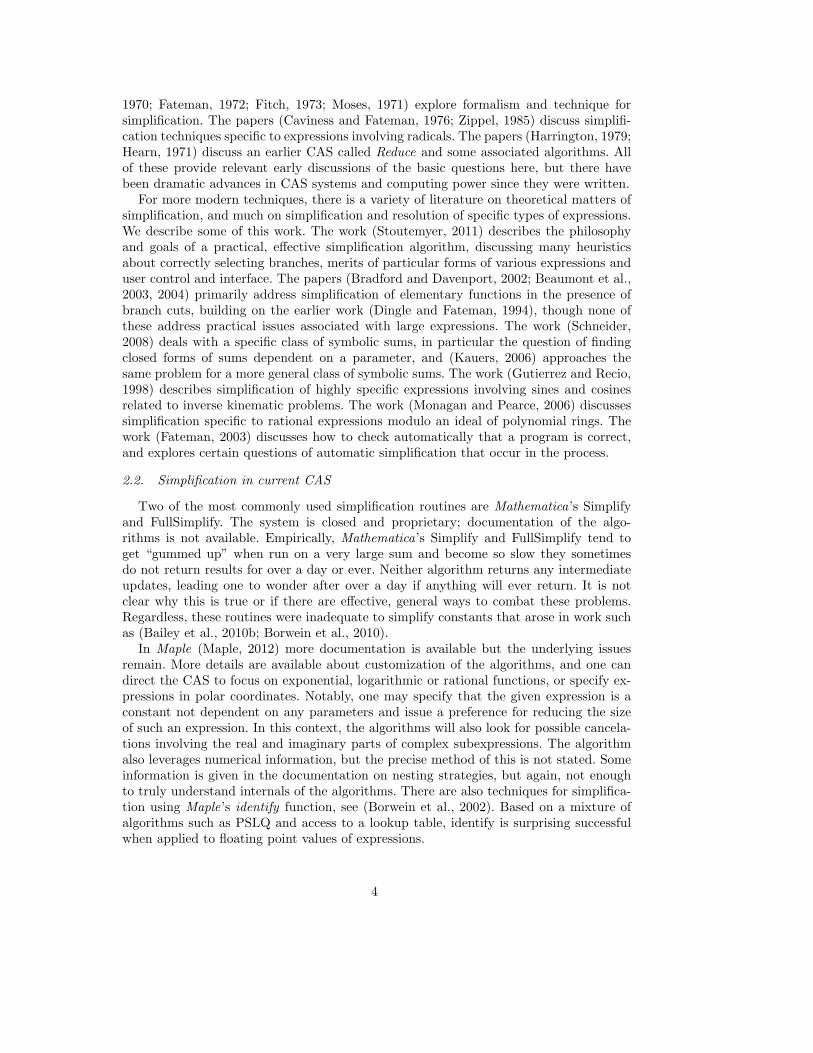
(1) First, redundancy is explored. The code compares all pairs to remove redundantequalities, opposites and complex conjugates. This O(n2) loop is robust at removingsuch elements, while more generic approaches may miss such relationships or simplyfail to function. The loop repeats until no change is detected. Pseudocode is shownin Algorithm 1.

Algorithm 1 Removal of redundancy1: repeat2: for all pairs of indices i, j do3: if (αixi == αjxj) || (|αixi − αjxj | < tol) then4: αi = 2αi5: Remove αjxj6: end if7: if (αixi == −αjxj) || (|αixi + αjxj | < tol) then8: Remove αixi and αjxj9: end if

10: if (αixi == αjxj) || (|re(αixi − αjxj)| < tol && |im(αixi + αjxj)| < tol )then

11: αixi = 2 re(αixi)12: Remove αjxj13: end if14: end for15: until no change has occurred

The first comparison in each if statement is Mathematica’s built-in, symbolicequality. The second is a numerical evaluation of the terms as written using built-in arbitrary precision arithmetic. The parameter tol is set to 10−digits, where digitsis user specified and has a default value 500.

5

The symbolic equality comparisons are in place because the user may wish toavoid numerical comparisons. It seems unlikely that the symbolic equality case willpass, because Mathematica will group terms automatically, but this does happen.We observed this behavior simplifying the constant J(2), which is discussed in sec-tion 5. The code includes switches to perform comparisons only with the symbolicor numerical comparisons, as desired.

Mathematica’s built in caching is used to avoid reevaluating expressions. Thefirst loop usually takes the majority of the time, since in the first evaluation noevaluations are cached.

There are algorithms that have a better asymptotic order, but the evaluationof each element is much more costly than looping over the list. Additionally, thisapproach is more resistant to bugs. We plan to explore approaches with a betterasymptotic complexity in the future.

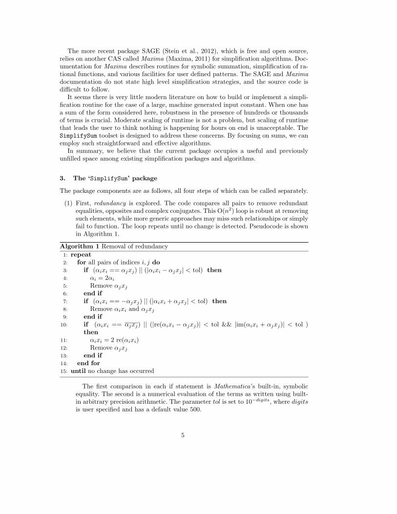
(2) Next are decomplexification routines to attempt to make constants real. The codelooks for terms that are stored as complex but have numerically zero imaginarypart. These are converted to real datatypes. This step is O(n). It then evaluatesremaining complex terms and converts them to real if their imaginary parts sum tozero. It removes them from the sum entirely if both the real and imaginary partssum to zero. This is unusual, but sometimes all the complex terms (not just theirimaginary parts) are extraneous results of a machine calculation. This is also O(n).Pseudocode is shown in Algorithm 2.

Algorithm 2 Decomplexification1: for i = 1:n do2: if |im(αixi)| < tol then3: αixi = re(αixi)4: end if5: end for6: Define E = {i : xi is complex}7: if |im

(∑i∈E αixi

)| < tol then

8: if | re(∑

i∈E αixi)| < tol then

9: Remove αixi for i ∈ E10: else11: Set αixi = re(αixi) for i ∈ E12: end if13: end if

This routine does not look at arbitrary combinations of elements, only singleelements and the whole sum. Note that removal of conjugate pairs in Algorithm 1is also decomplexification, and this examines all pairs but not all subsets.

(3) The code then performs an integer-relation detection step, using the multipairPSLQ algorithm (Bailey and Broadhurst, 2000) to remove dependent terms. Herewe use the notation zi = αixi for clarity.

An integer relation algorithm takes a vector of real or complex numbers (z1, z2 . . . zn)and attempts to find a nontrivial relationship

a1z1 + a2z2 + · · ·+ anzn = 0, (1)

6

where each ai is an integer. The multipair PSLQ algorithm, like any scheme forinteger relation detection, must be performed using at least (nd)-digit precision,where d is the size in digits of the largest of the coefficients ai, and n is the vec-tor length. See (Bailey and Broadhurst, 2000) for details on the multipair PSLQalgorithm.

If such a relationship is found, our code uses the simple identity

zi = −∑j,j 6=i ajzj

ai(2)

for some i such that ai 6= 0 to remove zi from the expression.The package repeatedly runs the multipair PSLQ algorithm to find relations. If a

relationship is found, a term is removed using equation (2), and then the algorithmis re-run, until no relations are found. The scheme can be run on the entire expres-sion, or some subset of the sum. The computer runtime of this algorithm increasesat least cubically with n, and even more rapidly if one takes into account the higherprecision needed for large n, so selecting a smaller subset is either essential or atleast beneficial in most cases.

Zero determination is treated separately. Instead of applying equation (2), thecode will also check for the fortunate circumstance that∑

i s.t.ai 6=0

zi = 0. (3)

or equivalently

ai ∈ {0, 1} for all i. (4)

That is, some combination of terms in the original equation simply summed tozero. In this case the appropriate zi are all removed. This is surprisingly commonin practice with machine generated constants. The problem of finding subsets whichsum to zero is formally NP-Complete, see (Lagarias and Odlyzko, 1985). PSLQ canfrequently find such relationships, even despite the complexity of the full formalproblem.

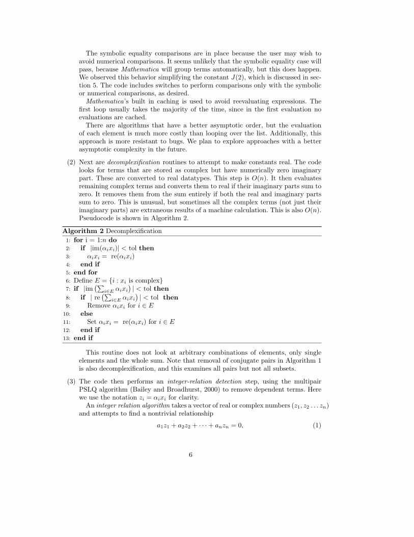
Pseudocode for integer-relation detection is shown in Algorithm 3.

Algorithm 3 Integer relation detection1: Select a subset of sum elements E and remove it from the sum.2: repeat3: Run multipair PSLQ to detect an integer relation4: if a relationship is found then5: if ai ∈ {0, 1} for all i then6: Remove all zi such that ai = 1. This is zero determination.7: else8: Apply equation (2) to remove a term from the sum.9: end if

10: end if11: until no relationship is found12: Replace the simplified E in the sum.

7

There are three strategies to pick subsets of the sum on which to run multipairPSLQ. First, relationships are much more likely to be found between terms thathave some mathematical relationship with each other. Thus, the code examinessubsets that are related according to user provided categories. For example, asin section 5, one may wish to group all terms with logarithms in one category,dilogarithms in another and so forth. If possible, this is the best strategy.

Another strategy is to make a randomized selection of terms. This may be ef-fective when little is known about the individual terms of the sum. If the user hasenough knowledge to determine categories a priori, then using that knowledge ismore effective. The final strategy is to simply run on adjacent blocks of the overallsum. This would seem less effective than randomized selection, but experience hasshown it is frequently better. Perhaps this is an artifact of another algorithm in themachine generated test constants. By default the code splits the sum into blocksof 10, 20 then 50 adjacent elements of the sum. It can also run on adjacent blockswithin categories.

By default, 500-digit arithmetic is used in the multipair PSLQ routine, and itis presumed that an identity that holds to 500-digit arithmetic is in fact a truemathematical identity, even though in a strict mathematical sense this cannot beguaranteed. If a higher level of certitude is desired, the precision level can be in-creased. However, Mathematica handles rational coefficients with exact, symbolicarithmetic. Thus, if the relationship is valid, there are no numerical errors madeperforming this substitution.

Relationships with too large a Euclidean norm are thrown out. The value is userspecified, with a low default value of 105. If a relation has large coefficients, thenapplying the relation may cause rational coefficients to get very large (in numberof digits in the numerator and denominator). This is the rare case discussed in theintroduction where growth in rational coefficients may increase the complexity ofan expression according to Carette’s formalism. This can be avoided by setting thebound lower, but then more relationships will be missed.

Note that all of the relationships in in Algorithm 1 could be found with multipairPSLQ. The disadvantage is speed, since multipair PSLQ has significant overheadcompared to adding or subtracting two constants.

(4) The final portion of the code is a substitution package.Mathematica uses objects called rules to perform a user specified substitution.

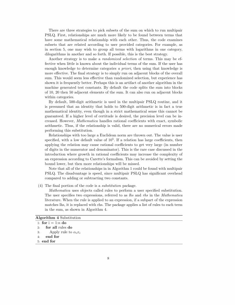
The user specifies two expressions, referred to as lhs and rhs in the Mathematicaliterature. When the rule is applied to an expression, if a subpart of the expressionmatches lhs, it is replaced with rhs. The package applies a list of rules to each termin the sum, as shown in Algorithm 4.

Algorithm 4 Substitution1: for i = 1:n do2: for all rules do3: Apply rule to αixi4: end for5: end for

8

This routine may or may not lead to simpler expressions. It follows the usersrequest even if this adds terms to the sum.

This makes O(nk) attempts at substitutions, where k is the number of rulesprovided. It operates on individual terms of the sum to maintain robustness onvery large sums. The Mathematica documentation pages have far more informationon the use of such substitutions. This is in contrast to built-in routines, whichthe Mathematica documentation says act on “every subpart of your expression.”Perhaps due to exponential growth in the number of terms in “every subpart” of asum, the built-in routine may run slowly. The routine here is strictly less powerfulthan the built-in substitution package, but runs faster on large expressions.

The package does not include any rules by default, all must be user-specified.Examples are included. Mathematica does not have any default rules, other thanwhat may be in Simplify or FullSimplify.

Remark 1 (Disclaimer). This combination of procedures can be very effective at remov-ing and simplifying terms. The user must, however, be mindful to consider the differencebetween numerical matches and true equality. Depending on the options used, numericalcomparisons may be used repeatedly as ‘truths’ in this package. Such output must, ofcourse not be taken as proof, only as experimental evidence. But in many applicationsthis may not matter, and in some others “knowledge is nine-tenths of a proof”. 3

Remark 2 (Precision). In many simplification algorithms of this type, incremental pre-cision is used. We leave this decision to the user. If one is satisfied with 100 digit precisionfor redundancy checking and decomplexification, these routines can be run at this level.Precision can then be increased to 500 or desired level for multipair PSLQ, which typicallyrequires higher precision. 3

4. Examples

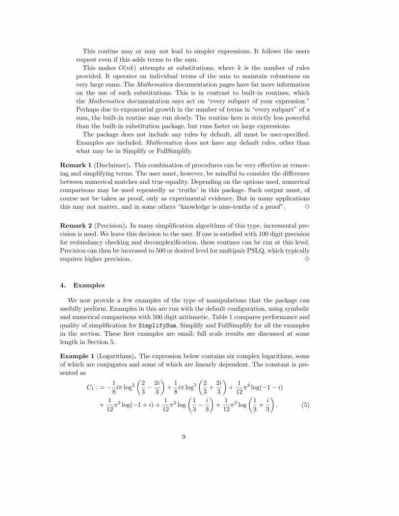
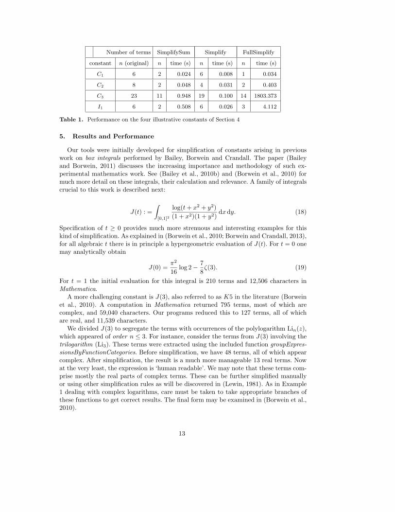
We now provide a few examples of the type of manipulations that the package canusefully perform. Examples in this are run with the default configuration, using symbolicand numerical comparisons with 500 digit arithmetic. Table 1 compares performance andquality of simplification for SimplifySum, Simplify and FullSimplify for all the examplesin the section. These first examples are small; full scale results are discussed at somelength in Section 5.

Example 1 (Logarithms). The expression below contains six complex logarithms, someof which are conjugates and some of which are linearly dependent. The constant is pre-sented as

C1 : = −18iπ log2

(23− 2i

3

)+

18iπ log2

(23

+2i3

)+

112π2 log(−1− i)

+112π2 log(−1 + i) +

112π2 log

(13− i

3

)+

112π2 log

(13

+i

3

). (5)

9

Redundancy checking finds three conjugate pairs and removes them.

2 re(−1

8iπ log2

(23− 2i

3

))+ 2 re

(112π2 log(−1− i)

)+ 2 re

(112π2 log

(13− i

3

))(6)

Integer relation detection finds the identity

8 re(−1

8iπ log2

(23− 2i

3

))+ 12 re

(112π2 log(−1− i)

)+ 6 re

(112π2 log

(13− i

3

))= 0

(7)

The package applies it to obtain

23

re(−1

8iπ log2

(23− 2i

3

))+ re

(112π2 log

(13− i

3

)). (8)

This in turn can be simplified by manually selecting the principal branch of log or usingFullSimplify.

Of course, correctly selecting branches require care, so the code does not perform thisparticular simplification unless an appropriate rule is set or calls to the Mathematicasimplify functions are made.

For comparison, Simplify removes zero terms and returns

124π

(2π(

log(−1− i) + log(−1 + i) + log(

13− i

3

)+ log

(13

+i

3

))(9)

−3i(

log2

(23− 2i

3

)− log2

(23

+2i3

))).

FullSimplify, however, correctly handles the branches and reduces to a single term.

− 148π2 log(18) (10)

This illustrates a weakness of the package. FullSimplify has a wider selection of trans-formations. If it is sufficiently fast, the results are better. Table 1 shows the number ofterms obtained by Simplify and FullSimplify. Timing on larger expressions shows thatFullSimplify is frequently slow, as discussed in section 5. 3

Example 2 (Arctangents). To illustrate the problem consider the arctangent identity

π

2− arctan

(√5)

= arctan

(3−√

54

)+ arctan

(√5− 2

),

which when expressed in terms of logarithms is

12i

(log(

1− 15i√

5)− log

(1 +

15i√

5))

(11)

=12i

(log(

1− 34i+

14i√

5)− log

(1 +

34i− 1

4i√

5))

(12)

+12i(

log(

1 + 2 i− i√

5)− log

(1− 2 i+ i

√5))

+14i log

(16 +

(√5− 3

)2)

. . .

10

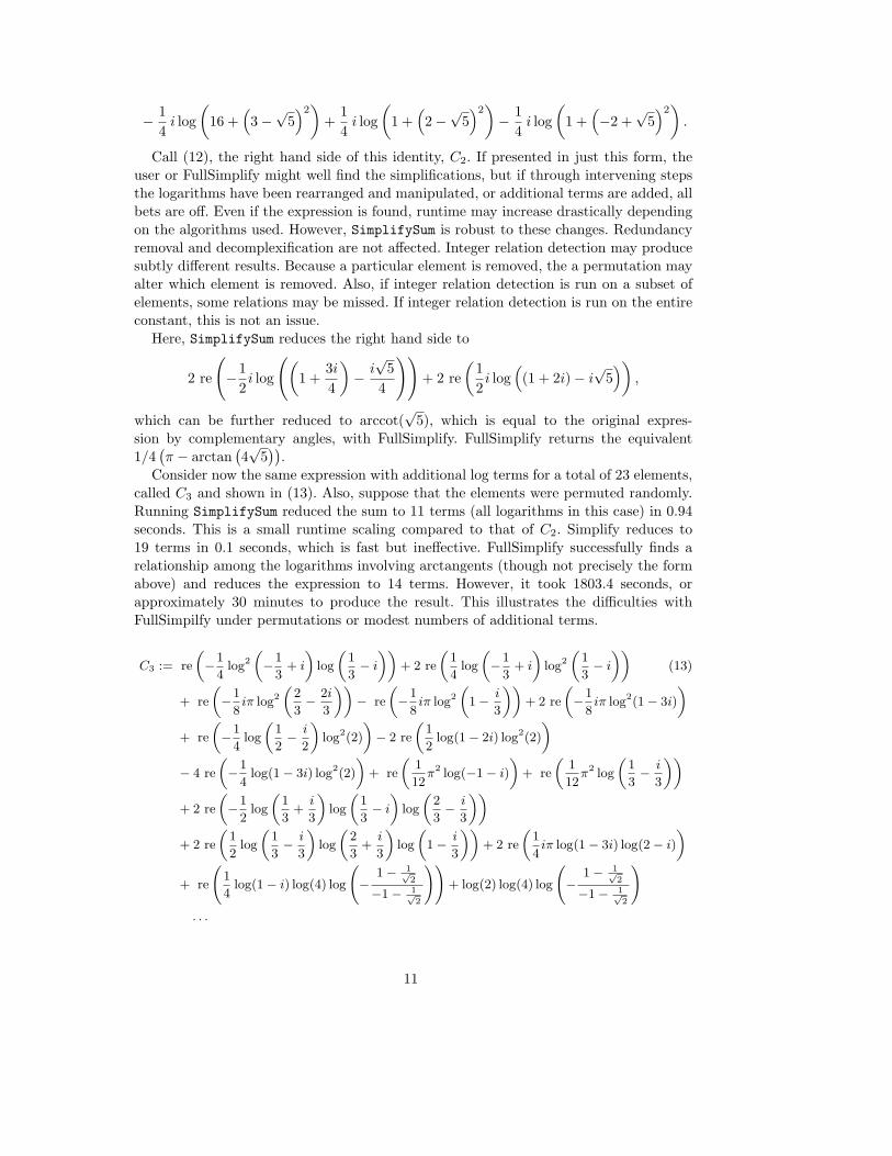
− 14i log

(16 +

(3−√

5)2)

+14i log

(1 +

(2−√

5)2)− 1

4i log

(1 +

(−2 +

√5)2).

Call (12), the right hand side of this identity, C2. If presented in just this form, theuser or FullSimplify might well find the simplifications, but if through intervening stepsthe logarithms have been rearranged and manipulated, or additional terms are added, allbets are off. Even if the expression is found, runtime may increase drastically dependingon the algorithms used. However, SimplifySum is robust to these changes. Redundancyremoval and decomplexification are not affected. Integer relation detection may producesubtly different results. Because a particular element is removed, the a permutation mayalter which element is removed. Also, if integer relation detection is run on a subset ofelements, some relations may be missed. If integer relation detection is run on the entireconstant, this is not an issue.

Here, SimplifySum reduces the right hand side to

2 re

(−1

2i log

((1 +

3i4

)− i√

54

))+ 2 re

(12i log

((1 + 2i)− i

√5))

,

which can be further reduced to arccot(√

5), which is equal to the original expres-sion by complementary angles, with FullSimplify. FullSimplify returns the equivalent1/4

(π − arctan

(4√

5))

.Consider now the same expression with additional log terms for a total of 23 elements,

called C3 and shown in (13). Also, suppose that the elements were permuted randomly.Running SimplifySum reduced the sum to 11 terms (all logarithms in this case) in 0.94seconds. This is a small runtime scaling compared to that of C2. Simplify reduces to19 terms in 0.1 seconds, which is fast but ineffective. FullSimplify successfully finds arelationship among the logarithms involving arctangents (though not precisely the formabove) and reduces the expression to 14 terms. However, it took 1803.4 seconds, orapproximately 30 minutes to produce the result. This illustrates the difficulties withFullSimpilfy under permutations or modest numbers of additional terms.

C3 := re

„−1

4log2

„−1

3+ i

«log

„1

3− i««

+ 2 re

„1

4log

„−1

3+ i

«log2

„1

3− i««

(13)

+ re

„−1

8iπ log2

„2

3− 2i

3

««− re

„−1

8iπ log2

„1− i

3

««+ 2 re

„−1

8iπ log2(1− 3i)

«+ re

„−1

4log

„1

2− i

2

«log2(2)

«− 2 re

„1

2log(1− 2i) log2(2)

«− 4 re

„−1

4log(1− 3i) log2(2)

«+ re

„1

12π2 log(−1− i)

«+ re

„1

12π2 log

„1

3− i

3

««+ 2 re

„−1

2log

„1

3+i

3

«log

„1

3− i«

log

„2

3− i

3

««+ 2 re

„1

2log

„1

3− i

3

«log

„2

3+i

3

«log

„1− i

3

««+ 2 re

„1

4iπ log(1− 3i) log(2− i)

«+ re

1

4log(1− i) log(4) log

−

1− 1√2

−1− 1√2

!!+ log(2) log(4) log

−

1− 1√2

−1− 1√2

!. . .

11

− 1

2i log

„„1 +

3i

4

«− i√

5

4

«+

1

2i log

„„1− 3i

4

«+i√

5

4

«+

1

2i log

“(1 + 2i)− i

√5”

− 1

2i log

“(1− 2i) + i

√5”

+1

4i log

„1 +

“2−√

5”2«− 1

4i log

„16 +

“3−√

5”2«

+1

4i log

„16 +

“√5− 3

”2«− 1

4i log

„1 +

“√5− 2

”2«.

Another technique is to apply FullSimplify to the reduced expression computed bySimplifySum. This took 35.9 seconds and reduces the output to 8 terms. This illustratesanother point — FullSimplify is a powerful routine, and sometimes the best result comesfrom applying SimplifySum and FullSimplify in combination. 3

Elaborate integrands can arise in high-end use of computer algebra packages. Manyof the following examples involve the polylogarithm Lin(z) :=

∑k≥1 x

k/kn of order n.(Note that Li1(x) = − log(1− x).)

Example 3 (Integrals I). Consider the following integral, which arose in connection tothe integral K1 in (Bailey et al., 2010a).∫ π/3

π/6

log(

2 sin(x

2

))dx (14)

Mathematica evaluates the integral symbolically to

I1 :=1

144

(− 144i

(Li2(

6√−1)− Li2

(3√−1))

+ 19iπ2

+ 12π(

log(2) + 2 log(1− 6√−1)− 2 log

(√3− 1

))). (15)

Here, Mathematica has produced complex subexpressions in evaluating an expressionthat is real. This is but one simple example of this phenomenon that occurs regularly incomputing integrals, including the following examples. After applying SimplifySum, wehave

re(−iLi2

(6√−1))

+ re(iLi2

(3√−1)). (16)

In this case, the imaginary parts sum to zero and are removed, removing one termentirely. PSLQ finds that three remaining terms sum to zero and are removed by zerodetermination. In contrast, FullSimplify reduces the original expression to

116i(16(Li2(

3√−1)− Li2

(6√−1))

+ π2), (17)

which has the disadvantage that it appears complex (though is also real) and has oneadditional term.

We note that if the user or system is aware of the literature on logsine integrals or theClausen function, Cl2(θ) = Im Li2

(eiθ)

(Borwein et al., 2012; Lewin, 1981), he or shewill immediately reduce (16) to Cl2(π/3) − Cl2(π/6). The package does not make suchsubstitutions automatically, because this would move the simplification process to thegeneral situation of (Carette, 2004). If desired, the user can use the substitution packageto apply them. 3

12

Number of terms SimplifySum Simplify FullSimplify

constant n (original) n time (s) n time (s) n time (s)

C1 6 2 0.024 6 0.008 1 0.034

C2 8 2 0.048 4 0.031 2 0.403

C3 23 11 0.948 19 0.100 14 1803.373

I1 6 2 0.508 6 0.026 3 4.112

Table 1. Performance on the four illustrative constants of Section 4

5. Results and Performance

Our tools were initially developed for simplification of constants arising in previouswork on box integrals performed by Bailey, Borwein and Crandall. The paper (Baileyand Borwein, 2011) discusses the increasing importance and methodology of such ex-perimental mathematics work. See (Bailey et al., 2010b) and (Borwein et al., 2010) formuch more detail on these integrals, their calculation and relevance. A family of integralscrucial to this work is described next:

J(t) : =∫

[0,1]2

log(t+ x2 + y2)(1 + x2)(1 + y2)

dxdy. (18)

Specification of t ≥ 0 provides much more strenuous and interesting examples for thiskind of simplification. As explained in (Borwein et al., 2010; Borwein and Crandall, 2013),for all algebraic t there is in principle a hypergeometric evaluation of J(t). For t = 0 onemay analytically obtain

J(0) =π2

16log 2− 7

8ζ(3). (19)

For t = 1 the initial evaluation for this integral is 210 terms and 12,506 characters inMathematica.

A more challenging constant is J(3), also referred to as K5 in the literature (Borweinet al., 2010). A computation in Mathematica returned 795 terms, most of which arecomplex, and 59,040 characters. Our programs reduced this to 127 terms, all of whichare real, and 11,539 characters.

We divided J(3) to segregate the terms with occurrences of the polylogarithm Lin(z),which appeared of order n ≤ 3. For instance, consider the terms from J(3) involving thetrilogarithm (Li3). These terms were extracted using the included function groupExpres-sionsByFunctionCategories. Before simplification, we have 48 terms, all of which appearcomplex. After simplification, the result is a much more manageable 13 real terms. Nowat the very least, the expression is ‘human readable’. We may note that these terms com-prise mostly the real parts of complex terms. These can be further simplified manuallyor using other simplification rules as will be discovered in (Lewin, 1981). As in Example1 dealing with complex logarithms, care must be taken to take appropriate branches ofthese functions to get correct results. The final form may be examined in (Borwein et al.,2010).

13

We observe that simple redundancies or branch issues such as illustrated in Example 3can and will replicate and grow unmanageably in large expansions such as the J integrals.

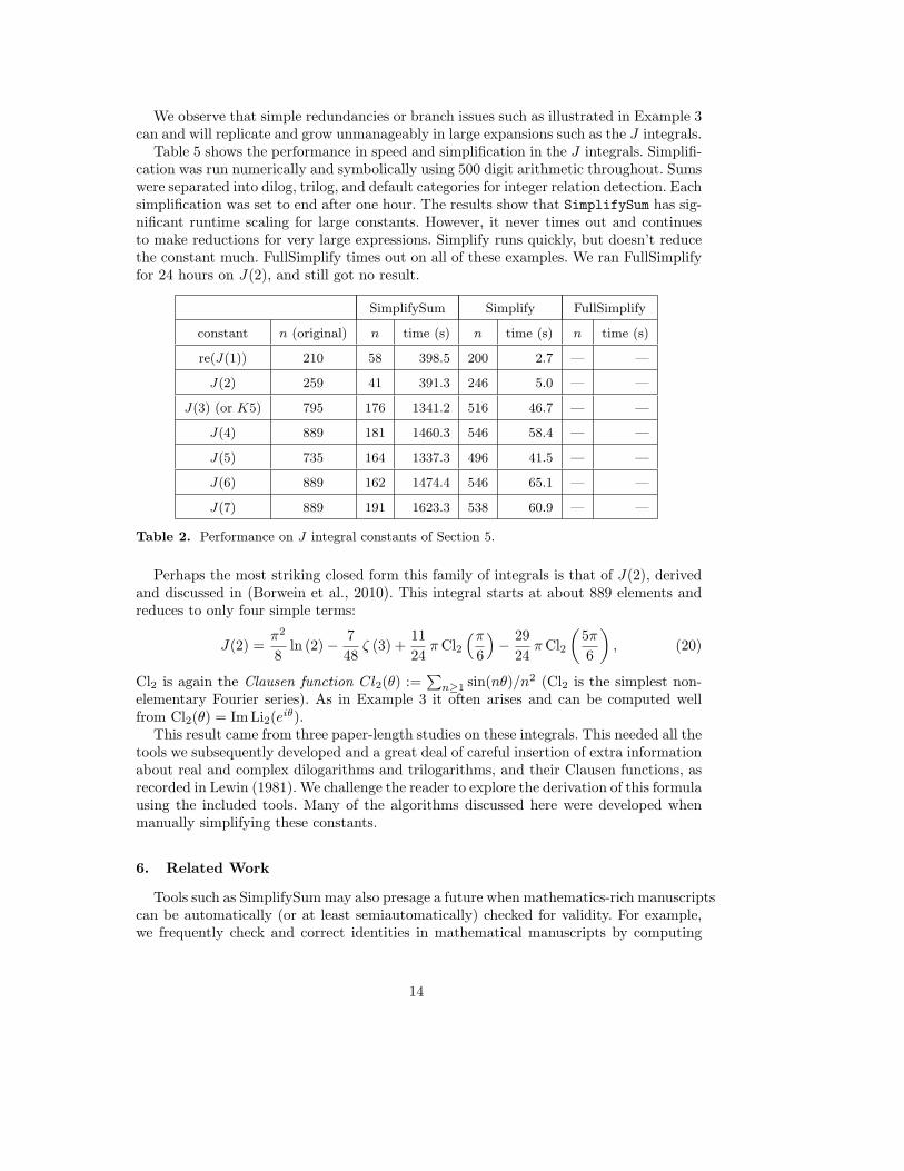
Table 5 shows the performance in speed and simplification in the J integrals. Simplifi-cation was run numerically and symbolically using 500 digit arithmetic throughout. Sumswere separated into dilog, trilog, and default categories for integer relation detection. Eachsimplification was set to end after one hour. The results show that SimplifySum has sig-nificant runtime scaling for large constants. However, it never times out and continuesto make reductions for very large expressions. Simplify runs quickly, but doesn’t reducethe constant much. FullSimplify times out on all of these examples. We ran FullSimplifyfor 24 hours on J(2), and still got no result.

SimplifySum Simplify FullSimplify

constant n (original) n time (s) n time (s) n time (s)

re(J(1)) 210 58 398.5 200 2.7 — —

J(2) 259 41 391.3 246 5.0 — —

J(3) (or K5) 795 176 1341.2 516 46.7 — —

J(4) 889 181 1460.3 546 58.4 — —

J(5) 735 164 1337.3 496 41.5 — —

J(6) 889 162 1474.4 546 65.1 — —

J(7) 889 191 1623.3 538 60.9 — —

Table 2. Performance on J integral constants of Section 5.

Perhaps the most striking closed form this family of integrals is that of J(2), derivedand discussed in (Borwein et al., 2010). This integral starts at about 889 elements andreduces to only four simple terms:

J(2) =π2

8ln (2)− 7

48ζ (3) +

1124πCl2

(π6

)− 29

24πCl2

(5π6

), (20)

Cl2 is again the Clausen function Cl2(θ) :=∑n≥1 sin(nθ)/n2 (Cl2 is the simplest non-

elementary Fourier series). As in Example 3 it often arises and can be computed wellfrom Cl2(θ) = Im Li2(eiθ).

This result came from three paper-length studies on these integrals. This needed all thetools we subsequently developed and a great deal of careful insertion of extra informationabout real and complex dilogarithms and trilogarithms, and their Clausen functions, asrecorded in Lewin (1981). We challenge the reader to explore the derivation of this formulausing the included tools. Many of the algorithms discussed here were developed whenmanually simplifying these constants.

6. Related Work

Tools such as SimplifySum may also presage a future when mathematics-rich manuscriptscan be automatically (or at least semiautomatically) checked for validity. For example,we frequently check and correct identities in mathematical manuscripts by computing

14

particular values on the LHS and RHS to high precision and comparing results—andthen if necessary use software to repair defects.

Remark 3. In much of our related work, we ultimately generate a significant numberof subtle formulas which end up as tabular data in a paper. While the formulas startas output of algorithms such as SimplifySum and are in principle symbolically correctand/or numerically validated identities, we realized than in the process of transcriptionand prettifying, errors are always introduced. For example in (Bailey et al., 2010b), 200formulas were collected, and 20 (or 10%) were found by our LaTeX to Mathematicaparser to be incorrect. A PSLQ based method was able to automatically correct 17 ofthese formulas. Of the remaining three, two were easy to debug by hand, while the finalone transpired to be humanly generated nonsense. We describe the methods below. 3

As an example, in a study of “character sums” we wished to use the following resultderived in (Borwein et al., 2008):

∞∑m=1

∞∑n=1

(−1)m+n−1

(2m− 1)(m+ n− 1)3(21)

?= 4 Li4

(12

)− 51

2880π4 − 1

6π2 log2(2) +

16

log4(2) +72

log(2)ζ(3).

Here Li4(1/2) is again a polylogarithmic value. However, a subsequent computation tocheck results disclosed that whereas the LHS evaluates to −0.872929289 . . ., the RHSevaluates to 2.509330815 . . .. Puzzled, we computed the sum, as well as each of the termson the RHS (sans their coefficients), to 500-digit precision, then applied the multipairPSLQ algorithm. Multipair PSLQ quickly found the following:

∞∑m=1

∞∑n=1

(−1)m+n−1

(2m− 1)(m+ n− 1)3(22)

= 4 Li4

(12

)− 151

2880π4 − 1

6π2 log2(2) +

16

log4(2) +72

log(2)ζ(3).

In other words, in the process of transcribing and ‘prettyfying’ (21) into the originalmanuscript, “151” had become “51.”

It is quite possible that this error would have gone undetected and uncorrected hadwe not been able to computationally check and correct such results. While any such errormay seem trivial, the reliability and integrity of tables and of resources like the DigitalLibrary of Mathematica Functions (Olver et al., 2012) demand such errors be identifiableand correctible. The ability to correct may not always matter, but it can be crucial.

We have largely automated these tools to validate and correct expressions, containedin a separate, in progress package titled VerifyEquality. We describe our code andunderlying heuristic in our final example, which arose in checking the paper (Bailey

15

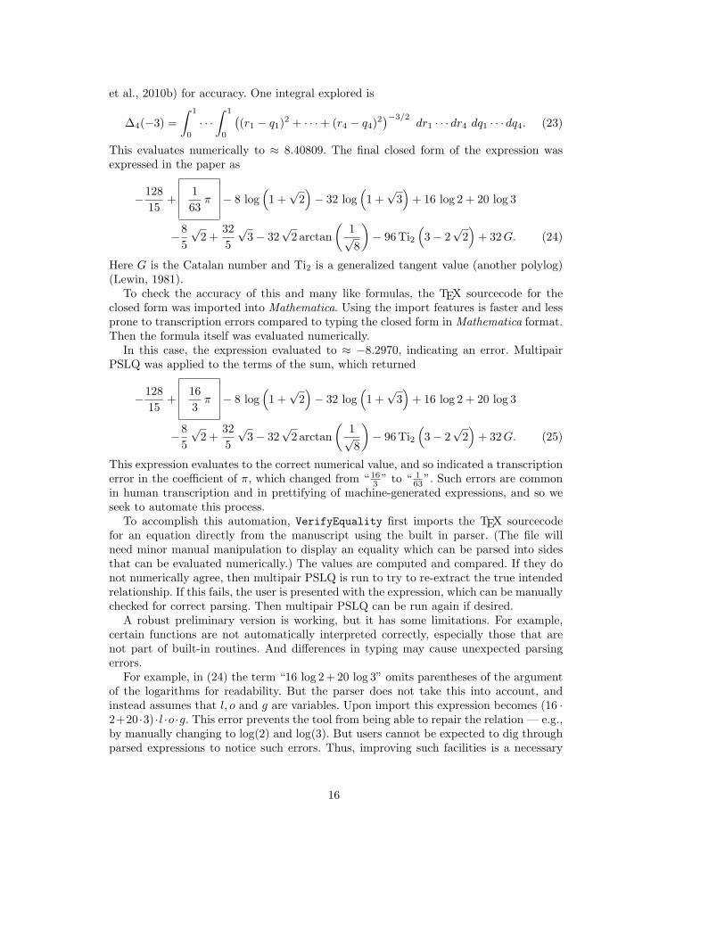
et al., 2010b) for accuracy. One integral explored is

∆4(−3) =∫ 1

0

· · ·∫ 1

0

((r1 − q1)2 + · · ·+ (r4 − q4)2

)−3/2dr1 · · · dr4 dq1 · · · dq4. (23)

This evaluates numerically to ≈ 8.40809. The final closed form of the expression wasexpressed in the paper as

−12815

+163π − 8 log

(1 +√

2)− 32 log

(1 +√

3)

+ 16 log 2 + 20 log 3

−85

√2 +

325

√3− 32

√2 arctan

(1√8

)− 96 Ti2

(3− 2

√2)

+ 32G. (24)

Here G is the Catalan number and Ti2 is a generalized tangent value (another polylog)(Lewin, 1981).

To check the accuracy of this and many like formulas, the TEX sourcecode for theclosed form was imported into Mathematica. Using the import features is faster and lessprone to transcription errors compared to typing the closed form in Mathematica format.Then the formula itself was evaluated numerically.

In this case, the expression evaluated to ≈ −8.2970, indicating an error. MultipairPSLQ was applied to the terms of the sum, which returned

−12815

+163π − 8 log

(1 +√

2)− 32 log

(1 +√

3)

+ 16 log 2 + 20 log 3

−85

√2 +

325

√3− 32

√2 arctan

(1√8

)− 96 Ti2

(3− 2

√2)

+ 32G. (25)

This expression evaluates to the correct numerical value, and so indicated a transcriptionerror in the coefficient of π, which changed from “ 16

3 ” to “ 163”. Such errors are common

in human transcription and in prettifying of machine-generated expressions, and so weseek to automate this process.

To accomplish this automation, VerifyEquality first imports the TEX sourcecodefor an equation directly from the manuscript using the built in parser. (The file willneed minor manual manipulation to display an equality which can be parsed into sidesthat can be evaluated numerically.) The values are computed and compared. If they donot numerically agree, then multipair PSLQ is run to try to re-extract the true intendedrelationship. If this fails, the user is presented with the expression, which can be manuallychecked for correct parsing. Then multipair PSLQ can be run again if desired.

A robust preliminary version is working, but it has some limitations. For example,certain functions are not automatically interpreted correctly, especially those that arenot part of built-in routines. And differences in typing may cause unexpected parsingerrors.

For example, in (24) the term “16 log 2 + 20 log 3” omits parentheses of the argumentof the logarithms for readability. But the parser does not take this into account, andinstead assumes that l, o and g are variables. Upon import this expression becomes (16 ·2+20 ·3) ·l ·o ·g. This error prevents the tool from being able to repair the relation — e.g.,by manually changing to log(2) and log(3). But users cannot be expected to dig throughparsed expressions to notice such errors. Thus, improving such facilities is a necessary

16

goal for full publication of this work. A further goal is to be able to automatically extractformulas from a paper, eliminating the need for users to manually annotate TEX sourcefiles.

Acknowledgements

The authors should like to thank Richard Crandall (now deceased) for his gracioushelp with sample constants. All feedback is appreciated. Comments on user experience,results, bug-reports, and results should be sent to adkaiser@gmail.com.

References

Bailey, D. H., Borwein, J. M., Nov. 2011. Exploratory experimentation and computation.Not. Amer. Math. Soc. 58, 1410–1419.

Bailey, D. H., Borwein, J. M., Broadhurst, D., Zudilin, W., 2010a. Experimental mathe-matics and mathematical physics. Gems in Exp. Math., Contemp. Math. 517, 41–58.

Bailey, D. H., Borwein, J. M., Crandall, R. E., 2010b. Advances in the theory of boxintegrals. Math. Comput. 79 (271), 1839–1866.URL http://dx.doi.org/10.1090/S0025-5718-10-02338-0

Bailey, D. H., Broadhurst, D. J., 2000. Parallel integer relation detection: Techniques andapplications. Math. Comput. 70, 1719–1736.

Beaumont, J., Bradford, R., Davenport, J. H., 2003. Better simplification of elementaryfunctions through power series. In: Proc. 2003 Int. Symp. on Symb. and Algebr. Comp.ISSAC ’03. ACM, New York, NY, USA, pp. 30–36.URL http://doi.acm.org/10.1145/860854.860867

Beaumont, J. C., Bradford, R. J., Davenport, J. H., Phisanbut, N., 2004. A poly-algorithmic approach to simplifying elementary functions. In: Proc. 2004 Int. Symp.on Symb. and Algebr. Comp. ISSAC ’04. ACM, New York, NY, USA, pp. 27–34.URL http://doi.acm.org/10.1145/1005285.1005292

Borwein, D., Borwein, J. M., Straub, A., Wan, J., In press 2012. Log-sine evaluations ofMahler measures, Part II. Integers.

Borwein, J. M., Chan, O.-Y., Crandall, R. E., 2010. Higher-dimensional box integrals.Exp. Math. 19 (4), 431–446.URL http://dx.doi.org/10.1080/10586458.2010.10390634

Borwein, J. M., Crandall, R. E., 2013. Closed forms: what they are and why we care.Not. Amer. Math. Soc. 60 (1).URL http://www.carma.newcastle.edu.au/jon/closed-form.pdf

Borwein, J. M., Zucker, I. J., Boersma, J., 2008. The evaluation of character Euler doublesums. Ramanujan J. 15, 377–405.

Borwein, P., Hare, K. G., Meichsner, A., 2002. Reverse symbolic computations, the iden-tify function. In: Maple Summer Workshop.

Bradford, R., Davenport, J. H., 2002. Towards better simplification of elementary func-tions. In: Proc. 2002 Int. Symp. on Symb. and Algebr. Comp. ISSAC ’02. ACM, NewYork, NY, USA, pp. 16–22.URL http://doi.acm.org/10.1145/780506.780509

17

Buchberger, B., Loos, R., 1982. Algebraic Simplification. In: Buchberger, B., Collins,G. E., Loos, R. (Eds.), Computer Algebra - Symbolic and Algebraic Computation.Springer Verlag, Vienna - New York, pp. 11–43.

Carette, J., 2004. Understanding expression simplification. In: Proc. 2004 Int. Symp. onSymb. and Algebr. Comp. ISSAC ’04. ACM, New York, NY, USA, pp. 72–79.URL http://doi.acm.org/10.1145/1005285.1005298

Casas, R., Fernandez-Camacho, M.-I., Steyaert, J.-M., 1990. Algebraic simplification incomputer algebra: an analysis of bottom-up algorithms. Theor. Comput. Sci. 74 (3),273–298.URL http://www.sciencedirect.com/science/article/pii/030439759090078V

Caviness, B. F., Apr. 1970. On canonical forms and simplification. J. ACM 17 (2), 385–396.URL http://doi.acm.org/10.1145/321574.321591

Caviness, B. F., Fateman, R. J., 1976. Simplification of radical expressions. In: Proc.third ACM Symp. on Symb. and Algebr. Comp. SYMSAC ’76. ACM, New York, NY,USA, pp. 329–338.URL http://doi.acm.org/10.1145/800205.806352

Chow, T. Y., 1999. What is a closed-form number? The American mathematical monthly106 (5), 440–448.

Dingle, A., Fateman, R. J., 1994. Branch cuts in computer algebra. In: Proc. 1994 Int.Symp. on Symb. and Algebr. Comp. ISSAC ’94. ACM, New York, NY, USA, pp. 250–257.URL http://doi.acm.org/10.1145/190347.190424

Fateman, R., 2003. High-level proofs of mathematical programs using automatic differ-entiation, simplification, and some common sense. In: Proc. 2003 Int. Symp. on Symb.and Algebr. Comp. ISSAC ’03. ACM, New York, NY, USA, pp. 88–94.URL http://doi.acm.org/10.1145/860854.860883

Fateman, R. J., 1972. Essays in algebraic simplification. Tech. rep., Cambridge, MA,USA.

Fitch, J. P., 1973. On algebraic simplification. The Comput. J. 16 (1), 23–27.URL http://comjnl.oxfordjournals.org/content/16/1/23.abstract

Gutierrez, J., Recio, T., 1998. Advances on the simplification of sinecosine equations. J.Symb. Comput. 26 (1), 31–70.URL http://www.sciencedirect.com/science/article/pii/S0747717198902000

Harrington, S. J., 1979. A new symbolic integration system in reduce. The Comput. J.22 (2), 127–131.URL http://comjnl.oxfordjournals.org/content/22/2/127.abstract

Hearn, A. C., 1971. Reduce 2: A system and language for algebraic manipulation. In:Proc. second ACM Symp. on Symb. and Algebr. Manip. SYMSAC ’71. ACM, NewYork, NY, USA, pp. 128–133.URL http://doi.acm.org/10.1145/800204.806277

Kauers, M., 2006. Sumcracker: A package for manipulating symbolic sums and relatedobjects. J. Symb. Comput. 41 (9), 1039–1057.URL http://www.sciencedirect.com/science/article/pii/S0747717106000502

Lagarias, J. C., Odlyzko, A. M., 1985. Solving low-density subset sum problems. Journalof the ACM (JACM) 32 (1), 229–246.

Lewin, L., 1981. Polylogarithms and associated functions. North Holland.

18

Maple, 2012. Maple. Maplesoft, Waterloo ON, Canada.URL http://www.maplesoft.com/support/help/Maple/view.aspx?path=simplify/details

Maxima, 2011. Maxima, a computer algebra system. version 5.25.1.URL http://maxima.sourceforge.net

Monagan, M., Pearce, R., 2006. Rational simplification modulo a polynomial ideal. In:Proc. 2006 Int. Symp. on Symb. and Algebr. Comp. ISSAC ’06. ACM, New York, NY,USA, pp. 239–245.URL http://doi.acm.org/10.1145/1145768.1145809

Moses, J., 1971. Algebraic simplification a guide for the perplexed. In: Proc. second ACMSymp. on Symb. and Algebr. Manip. SYMSAC ’71. ACM, New York, NY, USA, pp.282–304.URL http://doi.acm.org/10.1145/800204.806298

Olver, F. W. J., Lozier, D. W., Boisvert, R. F., Clark, C. W., 2012. NIST Digital Hand-book of Mathematical Functions.URL http://dlmf.nist.gov

Schneider, C., 2008. A refined difference field theory for symbolic summation. J. Symb.Comput. 43 (9), 611–644.URL http://www.sciencedirect.com/science/article/pii/S0747717108000047

Stein, W., et al., 2012. Sage Mathematics Software (Version 5.2). The Sage DevelopmentTeam.URL http://www.sagemath.org

Stoutemyer, D. R., 2011. Ten commandments for good default expression simplification.J. Symb. Comput. 46 (7), 859–887, special Issue in Honour of Keith Geddes on his60th Birthday.URL http://www.sciencedirect.com/science/article/pii/S0747717110001471

Zippel, R., 1985. Simplification of expressions involving radicals. J. Symb. Comput. 1 (2),189–210.URL http://www.sciencedirect.com/science/article/pii/S0747717185800146

7. Appendix

7.1. Included Files and Building

Download the source (available from https://github.com/alexkaiser/SimplifySum).Open Simplifysum.nb and evaluate all cells in the notebook. Two simple examplesare provided in Example.nb, and an example of using and writing rules is contained inRuleList.nb. Further examples from this paper are included in ExampleConstants.nband scripts to compare various simplifications are in TimingComparisons.nb

7.2. Basic usage

The most basic usage of the functions is to call the supplied ‘wrapper’ function withits default parameters unchanged. Name the constant that is to be simplified x. Thencall

simplifySum[x]This performs the following steps:

(1) Sets working precision to 500 digits.

19

(2) Removes terms that are equal, opposites or complex conjugates numerically andsymbolically. Performs the appropriate algebra symbolically to maintain equalityto the original sum.

(3) Converts complex terms that are numerically real to real datatypes.(4) Checks whether remaining complex terms sum to zero and delete them if so.(5) Check whether the imaginary part of remaining complex terms sum to zero and

make them real if so.(6) Repeatedly runs PSLQ on adjacent terms of the sum, removing and replacing terms

each time a relationship is found. Removes all terms in the sum in the event of zerodetermination.

(7) Checks accuracy and print a summary between each major step.(8) Returns the new expression.

7.3. Advanced usage

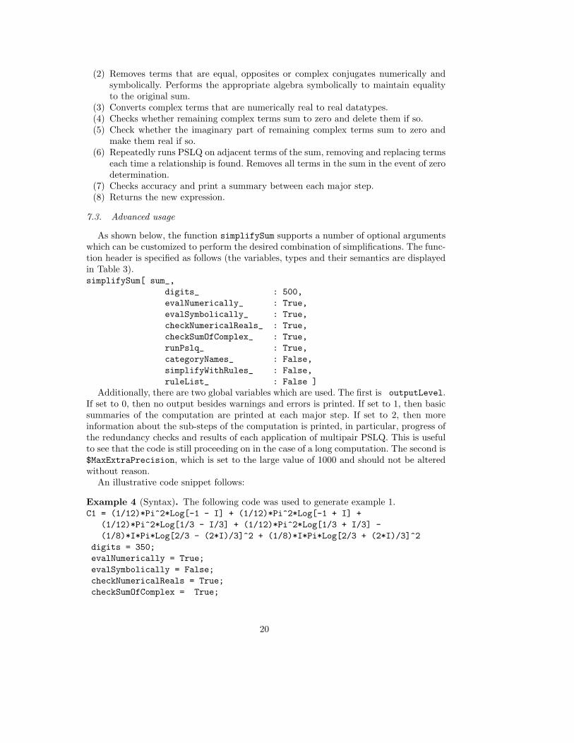
As shown below, the function simplifySum supports a number of optional argumentswhich can be customized to perform the desired combination of simplifications. The func-tion header is specified as follows (the variables, types and their semantics are displayedin Table 3).simplifySum[ sum_,

digits_ : 500,evalNumerically_ : True,evalSymbolically_ : True,checkNumericalReals_ : True,checkSumOfComplex_ : True,runPslq_ : True,categoryNames_ : False,simplifyWithRules_ : False,ruleList_ : False ]

Additionally, there are two global variables which are used. The first is outputLevel.If set to 0, then no output besides warnings and errors is printed. If set to 1, then basicsummaries of the computation are printed at each major step. If set to 2, then moreinformation about the sub-steps of the computation is printed, in particular, progress ofthe redundancy checks and results of each application of multipair PSLQ. This is usefulto see that the code is still proceeding on in the case of a long computation. The second is$MaxExtraPrecision, which is set to the large value of 1000 and should not be alteredwithout reason.

An illustrative code snippet follows:

Example 4 (Syntax). The following code was used to generate example 1.C1 = (1/12)*Pi^2*Log[-1 - I] + (1/12)*Pi^2*Log[-1 + I] +

(1/12)*Pi^2*Log[1/3 - I/3] + (1/12)*Pi^2*Log[1/3 + I/3] -(1/8)*I*Pi*Log[2/3 - (2*I)/3]^2 + (1/8)*I*Pi*Log[2/3 + (2*I)/3]^2

digits = 350;evalNumerically = True;evalSymbolically = False;checkNumericalReals = True;checkSumOfComplex = True;

20

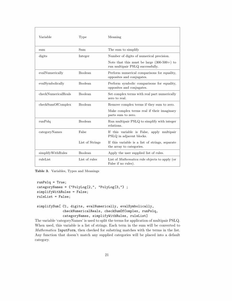
Variable Type Meaning

sum Sum The sum to simplify

digits Integer Number of digits of numerical precision.

Note that this must be large (300-500+) torun multipair PSLQ successfully.

evalNumerically Boolean Perform numerical comparisons for equality,opposites and conjugates.

evalSymbolically Boolean Perform symbolic comparisons for equality,opposites and conjugates.

checkNumericalReals Boolean Set complex terms with real part numericallyzero to real.

checkSumOfComplex Boolean Remove complex terms if they sum to zero.

Make complex terms real if their imaginaryparts sum to zero.

runPslq Boolean Run multipair PSLQ to simplify with integerrelations.

categoryNames False If this variable is False, apply multipairPSLQ in adjacent blocks.

List of Strings If this variable is a list of strings, separatethe array to categories.

simplifyWithRules Boolean Apply the user supplied list of rules.

ruleList List of rules List of Mathematica rule objects to apply (orFalse if no rules).

Table 3. Variables, Types and Meanings

runPslq = True;categoryNames = {"PolyLog[2,", "PolyLog[3,"} ;simplifyWithRules = False;ruleList = False;

simplifySum[ C1, digits, evalNumerically, evalSymbolically,checkNumericalReals, checkSumOfComplex, runPslq,categoryNames, simplifyWithRules, ruleList]

The variable ‘categoryNames’ is used to split the terms for application of multipair PSLQ.When used, this variable is a list of strings. Each term in the sum will be converted toMathematica InputForm, then checked for substring matches with the terms in the list.Any function that doesn’t match any supplied categories will be placed into a defaultcategory.

21

In this example, the categories are the ‘dilogarithm’ and ‘trilogarithm’, so those termswill each have their own category, while all other terms such as ordinary logarithms orany other known constants will be left in the default category.

The user should take care to consider name collisions, as a term will be placed onlyin the first match found or the default. 3

7.4. Final comments

The user may also wish to call the functions individually. Each function has its usage isdocumented in its its opening comments. Illustration of how to call individual functionsis included with function ‘simplifySum’.

Remark 4 (Simplification rules). If it is desired to simplify using or more user-definedrules, a function that applies those rules to each term in the sum is included. Recall thata Mathematica rule takes the following form:

old_expression :> new_expression /; conditionThe condition parameter is optional.

One should consult the examples included with our package or Mathematica’s owndocumentation on rules for more detail. As mentioned in section 3, the code here appliesrules to each element of the sum individually. If rules that effect more than one term ina sum are desired, then use the built in functions which operate on more levels of thesubexpressions.

That said, Mathematica does not divulge much in the way of documentation on itssource code. A direct request for more detail led to the response below:

“The general idea behind the Simplify and FullSimplify heuristics is that they apply asequence of transformations, keeping the version of the expression that has the smallestcomplexity found so far. This process is repeated at all subexpression levels.

There are a few thousand of transformations used (of course most of the transforma-tions apply to relatively narrow classes of expressions). We do not have documentationdescribing the transformations or the exact structure of the Simplify and FullSimplifyheuristics.”

An implementation in Maple or SAGE would thus be much more flexible. 3

8. Vitae

Can be supplied when and if needed.

22