Supplemental Information

High-content analysis screening for cell cycle regulators using arrayed synthetic crRNA libraries

Žaklina Strezoska, Matthew R. Perkett, Eldon T. Chou, Elena Maksimova, Emily M. Anderson, Shawn McClelland, Melissa L. Kelley, Annaleen Vermeulen, and Anja van Brabant Smith

Materials and methods

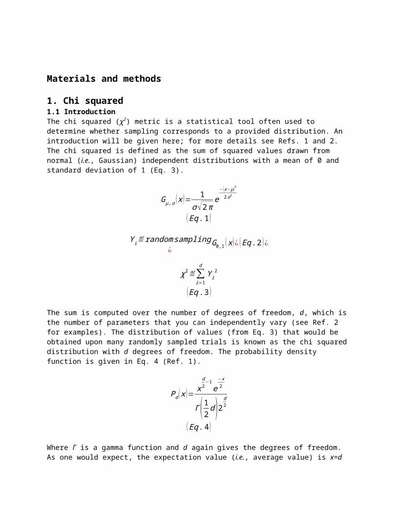
1. Chi squared1.1 IntroductionThe chi squared (χ2) metric is a statistical tool often used to determine whether sampling corresponds to a provided distribution. An introduction will be given here; for more details see Refs. 1 and 2. The chi squared is defined as the sum of squared values drawn from normal (i.e., Gaussian) independent distributions with a mean of 0 and standard deviation of 1 (Eq. 3).

Gμ ,σ ( x )= 1σ √2π

e−( x− μ)2

2σ2

(Eq .1 )

Y i≝random sampling¿

G0,1 ( x )¿ (Eq .2 )¿

χ2≝∑i=1

d

Y i2

(Eq .3 )

The sum is computed over the number of degrees of freedom, d, which is the number of parameters that you can independently vary (see Ref. 2 for examples). The distribution of values (from Eq. 3) that would be obtained upon many randomly sampled trials is known as the chi squared distribution with d degrees of freedom. The probability density function is given in Eq. 4 (Ref. 1).

Pd ( x )= xd2−1e

−x2

Γ ( 12 d )2d2

(Eq .4 )

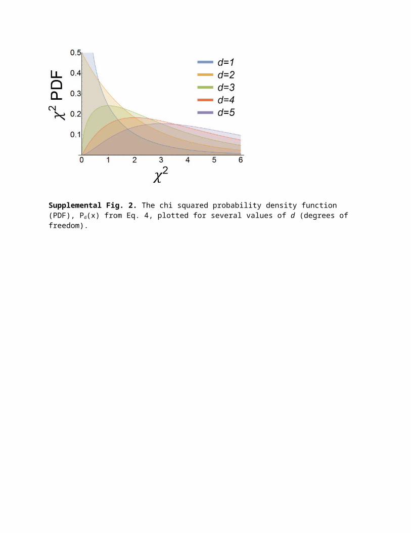
Where Γ is a gamma function and d again gives the degrees of freedom. As one would expect, the expectation value (i.e., average value) is x=d (see Supplemental Fig. 2 for Pd(x) plotted for multiple values of d). Having an equation for Pd(x) allows us to calculate a p-value for any given χ2 and d (i.e., the probability of obtaining a χ2 value or higher given d).

To permit simpler comparison between chi squared values, it is common practice to calculate the reduced chi squared, which gives the chi squared per degree of freedom.

reduced χ 2≝ χ2

d(Eq .5 )

It is worth noting that one cannot directly compare two reduced chi squared values if their degrees of freedom, d, differ.

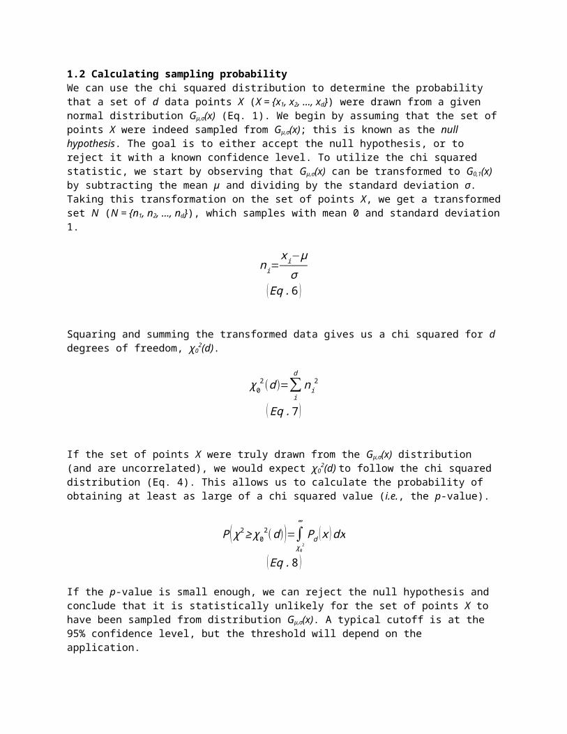
1.2 Calculating sampling probabilityWe can use the chi squared distribution to determine the probability that a set of d data points X (X = {x1, x2, ..., xd}) were drawn from a given normal distribution Gµ,σ(x) (Eq. 1). We begin by assuming that the set of points X were indeed sampled from Gµ,σ(x); this is known as the null hypothesis. The goal is to either accept the null hypothesis, or to reject it with a known confidence level. To utilize the chi squared statistic, we start by observing that Gµ,σ(x) can be transformed to G0,1(x) by subtracting the mean µ and dividing by the standard deviation σ. Taking this transformation on the set of points X, we get a transformed set N (N = {n1, n2, ..., nd}), which samples with mean 0 and standard deviation 1.

ni=x i−μσ

(Eq.6 )

Squaring and summing the transformed data gives us a chi squared for d degrees of freedom, χ02(d).

χ02(d)=∑

i

d

ni2

(Eq .7 )

If the set of points X were truly drawn from the Gµ,σ(x) distribution (and are uncorrelated), we would expect χ0

2(d) to follow the chi squared distribution (Eq. 4). This allows us to calculate the probability of obtaining at least as large of a chi squared value (i.e., the p-value).

P ( χ2≥ χ 02(d))=∫χ 02

∞

Pd ( x )dx

(Eq .8 )

If the p-value is small enough, we can reject the null hypothesis and conclude that it is statistically unlikely for the set of points X to have been sampled from distribution Gµ,σ(x). A typical cutoff is at the 95% confidence level, but the threshold will depend on the application.

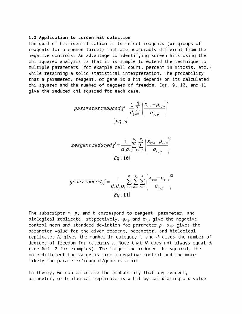
1.3 Application to screen hit selectionThe goal of hit identification is to select reagents (or groups of reagents for a common target) that are measurably different from the negative controls. An advantage to identifying screen hits using the chi squared analysis is that it is simple to extend the technique to multiple parameters (for example cell count, percent in mitosis, etc.) while retaining a solid statistical interpretation. The probability that a parameter, reagent, or gene is a hit depends on its calculated chi squared and the number of degrees of freedom. Eqs. 9, 10, and 11 give the reduced chi squared for each case.

parameter reduced χ2= 1db∑b=1

Nb

( xrpb−μc , pσc , p )2

(Eq .9 )

reagent reduced χ 2= 1d pdb

∑p=1

N p

∑b=1

Nb

( xrpb−μc , pσc , p )2

(Eq .10 )

genereduced χ 2= 1drd pdb

∑r=1

Nr

∑p=1

N p

∑b=1

Nb

( xrpb−μc , pσc , p )2

(Eq .11 )

The subscripts r, p, and b correspond to reagent, parameter, and biological replicate, respectively. µc,p and σc,p give the negative control mean and standard deviation for parameter p. xrpb gives the parameter value for the given reagent, parameter, and biological replicate. Ni gives the number in category i, and di gives the number of degrees of freedom for category i. Note that Ni does not always equal di (see Ref. 2 for examples). The larger the reduced chi squared, the more different the value is from a negative control and the more likely the parameter/reagent/gene is a hit.

In theory, we can calculate the probability that any reagent, parameter, or biological replicate is a hit by calculating a p-value (Eq. 8). In practice, several factors complicate this interpretation of the p-value, and hits are ranked by chi squared with a cutoff for significance chosen by other means (see the next section for a discussion on the complications). For example, we selected a cutoff at the gene level by identifying the gene with the largest reduced chi squared that was not expressed according to RNA-seq data.

1.4 Chi squared analysis assumptionsThere are several key assumptions to using the chi squared analysis as a strict statistical tool.

1. The negative control distribution is Gaussian for each parameter. For the transformation in Eq. 6 to make sense, the distribution must be approximately Gaussian.

2. Parameters are not correlated. The chi squared distribution assumes independently distributed values.

3. Negative controls are indicative of all “nonhits.” Otherwise, the chi squared will only indicate how unlike the chosen controls it is. Although this is very likely to be a good metric for ranking hits, the p-value no longer provides the probability that a reagent or gene is a “hit.”

Note that there is no assumption about the form of the distribution for screen parameters, but only for the negative controls. These assumptions can be relaxed if they are approximately true and one is willing to give up the strict interpretation of the p-value (Eq. 8). In this case, hits are identified by ranking reagents/genes by p-value and determining the significance threshold by other means (e.g., an RNA-seq cutoff as used in this study). Plots showing the negative control distribution for each parameter can be found in the Supplementary Data.

1.5 Additional considerationsParameters that are distributionsIn this study, we classified the cells in a well into one of six categories and used the percentage of cells in each category (and the total cell count) for the chi squared analysis. These parameters all naturally give

a single value per well, for example the percentage of cells in mitosis. However, one might also have a full distribution for a measured parameter (e.g., when measuring the form factor). The chi squared analysis outlined here will work without modification if a parameter’s distribution can be summarized by single parameters such as a distribution average and/or higher moments of the distribution (standard deviation, etc.). However, there may be situations where it is difficult or inappropriate to reduce a distribution in this way (e.g., taking the average for a bimodal distribution does not make sense). One approach is to bin the data from the distribution and use the chi squared statistic on each bin (see Ref. 2 for examples). Another approach may be to use a Kolmogorov-Smirnov (or similar) test as a metric for how similar the sampled distribution is to that of the negative controls.

Non-Gaussian negative controls The chi squared analysis assumes that the negative control parameters are at least approximately Gaussian, which is true for the screening data presented here. However, it is certainly possible to encounter a negative control parameter that is decidedly non-Gaussian (e.g., a bimodal distribution). One workaround is to calculate a parameter (or parameters) from the non-Gaussian parameter that is normally distributed (e.g., by separating the two peaks in a bimodal distribution). A more complex approach is to calculate an empirical “chi squared”-like statistic from the non-Gaussian parameter programmatically.

2. Comparison to an alternate hit identification methodThis section compares the chi squared analysis used in this study to a hit identification technique commonly used in the screening community (mean ± k standard deviations) extended to a multiparameter assay.

2.1 Hit identificationFor an assay with a single parameter, hits are ranked by the number of (negative control) standard deviations they are above the negative control mean. As is the case for other popular methods, it is ambiguous how to extend this technique to multiple parameters. Taking an average over all parameters to determine whether a reagent is a hit is a logical and simple choice, but it sacrifices the original interpretation (i.e., this no longer has a corresponding p-value). An alternative approach is to calculate the probability of obtaining seven such number of standard deviations measurements, which becomes significantly more complicated. To provide a simple and intuitive example for comparison, we decided to take the former approach.

This method identifies hits by counting the number of negative control standard deviations the screen parameter mean is from the negative control mean (ωgrp in the Eq 12).

ωgrp=μgrp−μc , pσc , p

(Eq .12 )

µgrp is the mean of the sample for gene g, reagent r, and parameter p. µc,p and σc,p give the mean and standard deviation (respectively) of the negative controls for parameter p. The sign of ωgrp gives whether the sample is above/below the negative control, and the greater |ωgrp|, the more likely it is a “hit.” In Eq. 12, we divide by the negative control’s standard deviation rather than the sample’s standard

deviation because it is known to a much higher degree of accuracy and less prone to random fluctuations (54 negative control data points vs. 3 data points per screened gene).

Reagent and gene level hits were then ranked by ωgr and ωg (respectively), a metric obtained by averaging |ωgrp| over the reagent/gene.

ωgr=1N p

∑p=1

N p

|ωgrp|(Eq .13 )

ωg=1

N r N p∑r=1

Nr

∑p=1

N p

|ωgrp|(Eq .14 )

Np and Nr give the number of parameters and number of reagents (respectively). The significance cutoff for ωg can be determined using the same criteria as for the chi squared analysis, but here we are only interested in the gene/reagent hit ranking for comparison.

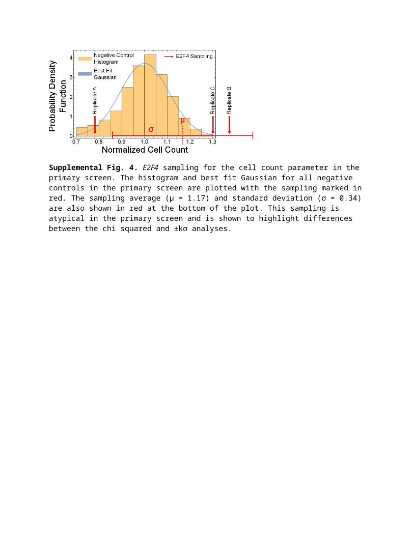
2.2 Fundamental difference from chi squaredAlthough the results from the two methods agree remarkably well for this screen, a fundamental difference between the two analyses can be explained by considering an extreme outlier, such as gene E2F4 crRNA 3 in the primary screen shown in Supplemental Fig. 4. This is clearly atypical sampling; two of the sampled data points are greater than measured for any of the 216 negative controls, and the third sample is about 2σ below the negative control mean. In the mean ± k standard deviations analysis, this parameter is a nonhit with the following justification: the spread in the sampling is large and so too must be the error; therefore, we cannot conclude much based on this data. On the other hand, the chi squared analysis marks this parameter as a fairly strong hit with the following rationale: 1. The goal of hit identification is to determine whether the sampling is measurably different from a negative control, 2. Based on the sampling, it is statistically very unlikely to be a negative control, 3. Since we cannot distinguish between bad sampling (i.e., an uninteresting systematic error) and a bimodal distribution centered at 0.8 and 1.3 with only three data points, this should be considered a hit. The chi squared analysis makes no assumptions about the sampling distribution for parameters in the screen and is less likely to miss potential hits. Confirmation of phenotype will separate true hits with atypical sampling from false positives. Sampling such as shown in Supplemental Fig. 4 was rare in this assay, but it provides insight into the chi squared analysis method.

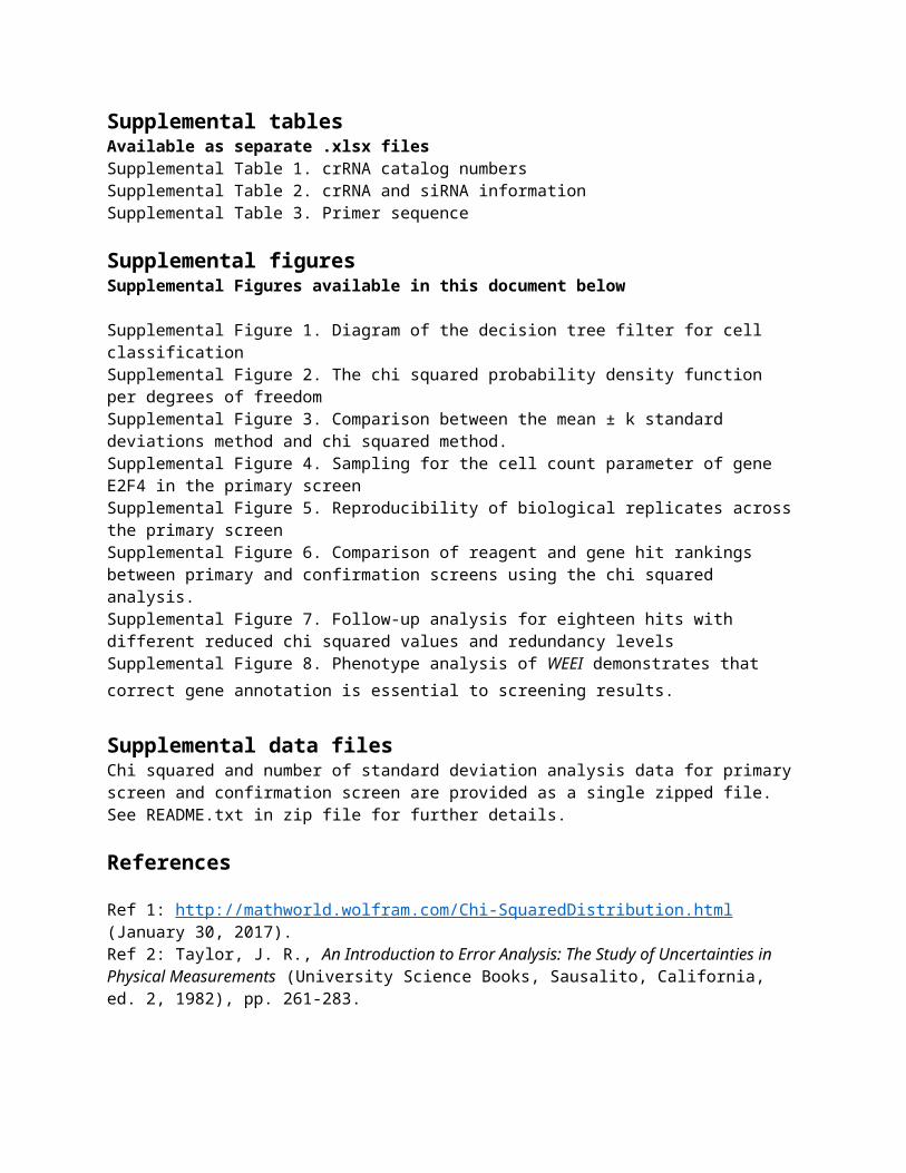
Supplemental tablesAvailable as separate .xlsx files Supplemental Table 1. crRNA catalog numbers Supplemental Table 2. crRNA and siRNA information Supplemental Table 3. Primer sequence

Supplemental figuresSupplemental Figures available in this document below

Supplemental Figure 1. Diagram of the decision tree filter for cell classificationSupplemental Figure 2. The chi squared probability density function per degrees of freedomSupplemental Figure 3. Comparison between the mean ± k standard deviations method and chi squared method.Supplemental Figure 4. Sampling for the cell count parameter of gene E2F4 in the primary screenSupplemental Figure 5. Reproducibility of biological replicates across the primary screenSupplemental Figure 6. Comparison of reagent and gene hit rankings between primary and confirmation screens using the chi squared analysis.Supplemental Figure 7. Follow-up analysis for eighteen hits with different reduced chi squared values and redundancy levelsSupplemental Figure 8. Phenotype analysis of WEEI demonstrates that correct gene annotation is essential to screening results.

Supplemental data filesChi squared and number of standard deviation analysis data for primary screen and confirmation screen are provided as a single zipped file. See README.txt in zip file for further details.

References

Ref 1: http://mathworld.wolfram.com/Chi-SquaredDistribution.html (January 30, 2017).Ref 2: Taylor, J. R., An Introduction to Error Analysis: The Study of Uncertainties in Physical Measurements (University Science Books, Sausalito, California, ed. 2, 1982), pp. 261-283.Ref 3: http://mathworld.wolfram.com/SpearmanRankCorrelationCoefficient.html (January 30, 2017).Ref 4: https://docs.scipy.org/doc/scipy-0.14.0/reference/generated/scipy.stats.spearmanr.html (January 30, 2017).

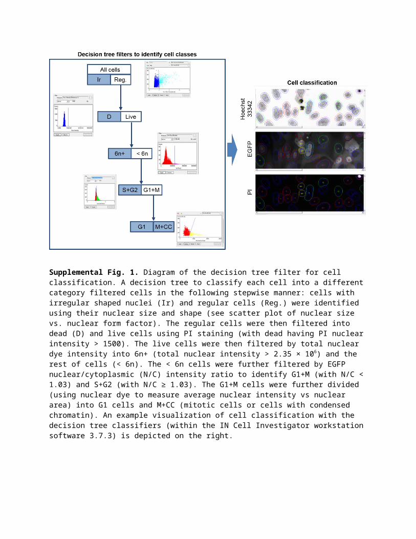
Supplemental Fig. 1. Diagram of the decision tree filter for cell classification. A decision tree to classify each cell into a different category filtered cells in the following stepwise manner: cells with irregular shaped nuclei (Ir) and regular cells (Reg.) were identified using their nuclear size and shape (see scatter plot of nuclear size vs. nuclear form factor). The regular cells were then filtered into dead (D) and live cells using PI staining (with dead having PI nuclear intensity > 1500). The live cells were then filtered by total nuclear dye intensity into 6n+ (total nuclear intensity > 2.35 × 106) and the rest of cells (< 6n). The < 6n cells were further filtered by EGFP nuclear/cytoplasmic (N/C) intensity ratio to identify G1+M (with N/C < 1.03) and S+G2 (with N/C ≥ 1.03). The G1+M cells were further divided (using nuclear dye to measure average nuclear intensity vs nuclear area) into G1 cells and M+CC (mitotic cells or cells with condensed chromatin). An example visualization of cell classification with the decision tree classifiers (within the IN Cell Investigator workstation software 3.7.3) is depicted on the right.

Supplemental Fig. 2. The chi squared probability density function (PDF), Pd(x) from Eq. 4, plotted for several values of d (degrees of freedom).

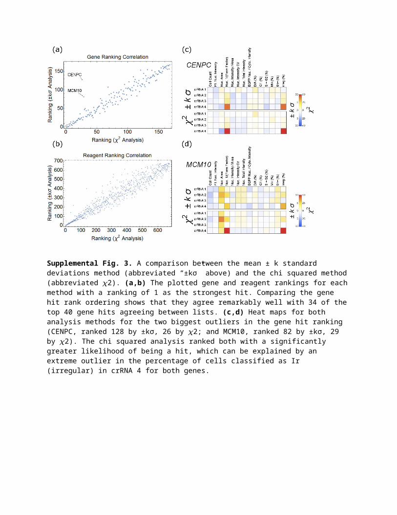
Supplemental Fig. 3. A comparison between the mean ± k standard deviations method (abbreviated “±kσ” above) and the chi squared method (abbreviated 𝜒2). (a,b) The plotted gene and reagent rankings for each method with a ranking of 1 as the strongest hit. Comparing the gene hit rank ordering shows that they agree remarkably well with 34 of the top 40 gene hits agreeing between lists. (c,d) Heat maps for both analysis methods for the two biggest outliers in the gene hit ranking (CENPC, ranked 128 by ±kσ, 26 by 𝜒2; and MCM10, ranked 82 by ±kσ, 29 by 𝜒2). The chi squared analysis ranked both with a significantly greater likelihood of being a hit, which can be explained by an extreme outlier in the percentage of cells classified as Ir (irregular) in crRNA 4 for both genes.

Supplemental Fig. 4. E2F4 sampling for the cell count parameter in the primary screen. The histogram and best fit Gaussian for all negative controls in the primary screen are plotted with the sampling marked in red. The sampling average (µ = 1.17) and standard deviation (σ = 0.34) are also shown in red at the bottom of the plot. This sampling is atypical in the primary screen and is shown to highlight differences between the chi squared and ±kσ analyses.

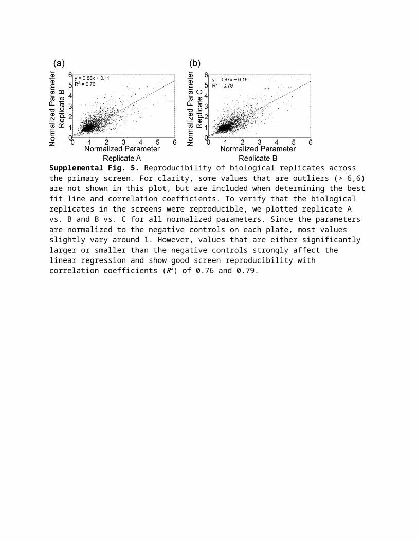
Supplemental Fig. 5. Reproducibility of biological replicates across the primary screen. For clarity, some values that are outliers (> 6,6) are not shown in this plot, but are included when determining the best fit line and correlation coefficients. To verify that the biological replicates in the screens were reproducible, we plotted replicate A vs. B and B vs. C for all normalized parameters. Since the parameters are normalized to the negative controls on each plate, most values slightly vary around 1. However, values that are either significantly larger or smaller than the negative controls strongly affect the linear regression and show good screen reproducibility with correlation coefficients (R2) of 0.76 and 0.79.

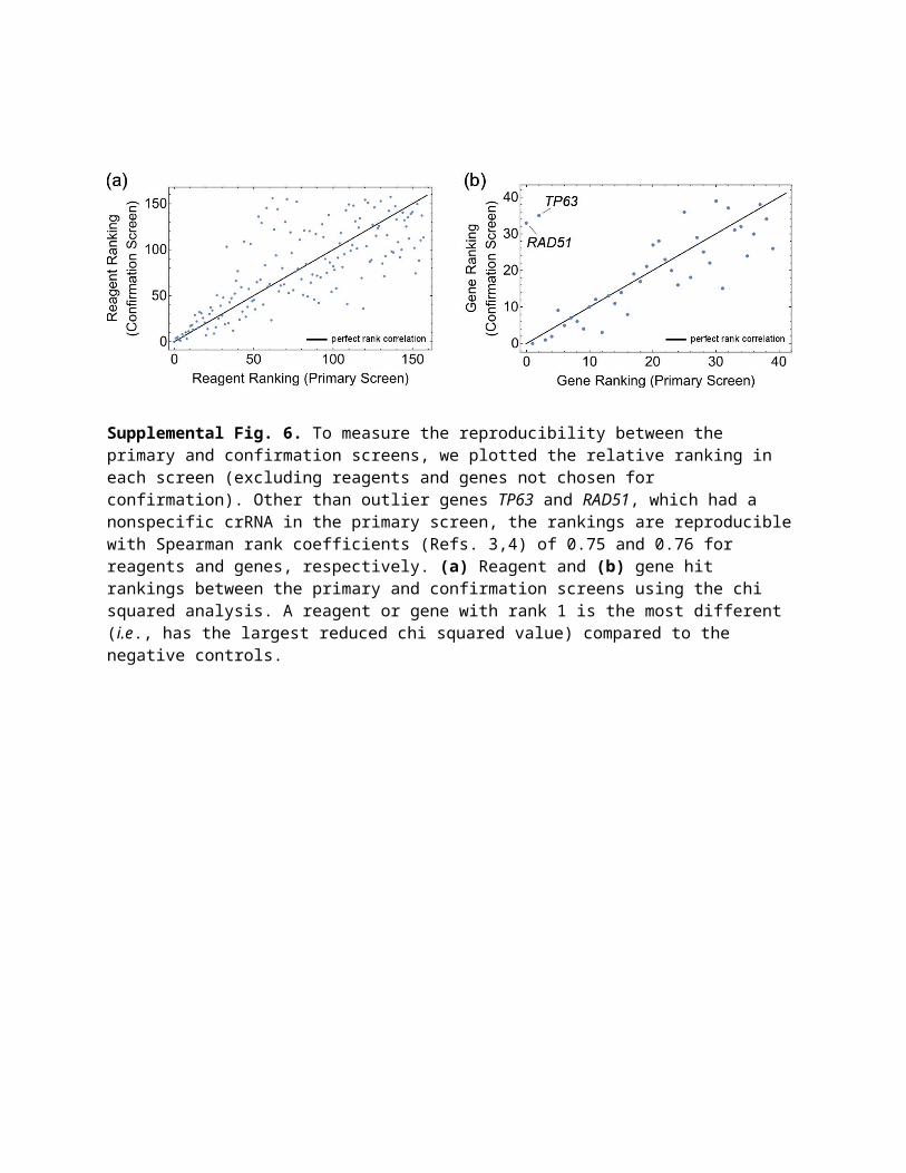
Supplemental Fig. 6. To measure the reproducibility between the primary and confirmation screens, we plotted the relative ranking in each screen (excluding reagents and genes not chosen for confirmation). Other than outlier genes TP63 and RAD51, which had a nonspecific crRNA in the primary screen, the rankings are reproducible with Spearman rank coefficients (Refs. 3,4) of 0.75 and 0.76 for reagents and genes, respectively. (a) Reagent and (b) gene hit rankings between the primary and confirmation screens using the chi squared analysis. A reagent or gene with rank 1 is the most different ( i.e., has the largest reduced chi squared value) compared to the negative controls.

(a)

(b)

Supplemental Fig. 7. Follow-up analysis for eighteen hits with different reduced chi squared values and redundancy levels. (a) Editing efficiency estimations by a mismatch detection assay using T7EI. (b) Reduced chi squared heat map representations of the HCA cell classification parameters for confirmed crRNA hits, with heat maps from the siRNA transfection experiment as a comparison. Blue is significantly below the NTC average value and red is significantly above the NTC average value for each parameter.

Supplemental Fig. 8. Phenotypic analysis of WEE1 demonstrates that correct gene annotation is essential to screening results. U2OS-Cas9 stable cells were transfected with different crRNAs targeting the WEE1 gene or an NTC crRNA control; induction of apoptosis was assayed 48hrs post-transfection using the Apo-ONE assay. Data was normalized as fold Apo-ONE signal over the NTC control. WEE1 crRNAs 1-3 were found to target before the annotated transcription start site in an updated RefSeq 80 and therefore did not show phenotypic response in the cell cycle HCA analysis. When tested with additional crRNAs (crRNAs 5-8) that target in the currently annotated CDS, all four of these crRNAs exhibit a phenotype in the Apo-ONE assay.