ANGLE MODULATION - جامعة بابل | University of Babylon maximum (or peak) radian frequency...

[4.1]

Dr. Ahmed A. Alrekaby

ANGLE MODULATION U1. PHASE AND FREQUENCY MODULATION

For angle modulation, the modulated carrier is represented by

𝑥𝑥𝑐𝑐(𝑡𝑡) = 𝐴𝐴 𝑐𝑐𝑐𝑐𝑐𝑐[𝜔𝜔𝑐𝑐𝑡𝑡 + 𝜙𝜙(𝑡𝑡)] (1.1)

Where A and ωc are constants and the phase angle 𝜙𝜙(𝑡𝑡) is a function of the message signal m(t). Equation (1.1) can be written as

𝑥𝑥𝑐𝑐(𝑡𝑡) = 𝐴𝐴 𝑐𝑐𝑐𝑐𝑐𝑐 𝜃𝜃(𝑡𝑡)

where 𝜃𝜃(𝑡𝑡) = 𝜔𝜔𝑐𝑐𝑡𝑡 + 𝜙𝜙(𝑡𝑡)

The instantaneous radian frequency of xc(t), denoted by ωi is

𝜔𝜔𝑖𝑖 =𝑑𝑑 𝜃𝜃(𝑡𝑡)𝑑𝑑𝑡𝑡 = 𝜔𝜔𝑐𝑐 +

𝑑𝑑 𝜙𝜙(𝑡𝑡)𝑑𝑑𝑡𝑡 (1.2)

𝜙𝜙(𝑡𝑡) = instantaneous phase deviation.

𝑑𝑑 𝜙𝜙(𝑡𝑡)𝑑𝑑𝑡𝑡 = instantaneous frequancy deviation.

The maximum (or peak) radian frequency deviation of the angle-modulated signal (∆ω) is given by

Δ𝜔𝜔 = |𝜔𝜔𝑖𝑖 − 𝜔𝜔𝑐𝑐 |𝑚𝑚𝑚𝑚𝑥𝑥 (1.3)

In phase modulation (PM) the instantaneous phase deviation of the carrier is proportional to the message signal; that is,

𝜙𝜙(𝑡𝑡) = 𝑘𝑘𝑝𝑝𝑚𝑚(𝑡𝑡) (1.4)

where kp is the phase deviation constant, expressed in radians per unit of m(t). In frequency modulation (FM), the instantaneous frequency deviation of the carrier is proportional to the message signal; that is,

𝑑𝑑 𝜙𝜙(𝑡𝑡)𝑑𝑑𝑡𝑡 = 𝑘𝑘𝑓𝑓𝑚𝑚(𝑡𝑡) (1.5𝑚𝑚)

or 𝜙𝜙(𝑡𝑡) = 𝑘𝑘𝑓𝑓 ∫ 𝑚𝑚(𝜆𝜆) 𝑑𝑑𝜆𝜆 (1.5𝑏𝑏)𝑡𝑡−∞

thus, we can express the angle-modulated signal as

𝑥𝑥𝑃𝑃𝑃𝑃(𝑡𝑡) = 𝐴𝐴 𝑐𝑐𝑐𝑐𝑐𝑐 [𝜔𝜔𝑐𝑐𝑡𝑡 + 𝑘𝑘𝑃𝑃𝑚𝑚(𝑡𝑡)] (1.6)

𝑥𝑥𝐹𝐹𝑃𝑃(𝑡𝑡) = 𝐴𝐴 𝑐𝑐𝑐𝑐𝑐𝑐 �𝜔𝜔𝑐𝑐𝑡𝑡 + 𝑘𝑘𝑓𝑓 � 𝑚𝑚(𝜆𝜆)𝑡𝑡

−∞𝑑𝑑𝜆𝜆� (1.7)

From Eq.(1.2),we have

[4.2]


𝜔𝜔𝑖𝑖 = 𝜔𝜔𝑐𝑐 + 𝑘𝑘𝑝𝑝𝑑𝑑 𝑚𝑚(𝑡𝑡)𝑑𝑑𝑡𝑡 𝑓𝑓𝑐𝑐𝑓𝑓 𝑃𝑃𝑃𝑃 (1.8)

𝜔𝜔𝑖𝑖 = 𝜔𝜔𝑐𝑐 + 𝑘𝑘𝑓𝑓𝑚𝑚(𝑡𝑡) 𝑓𝑓𝑐𝑐𝑓𝑓 𝐹𝐹𝑃𝑃 (1.9)

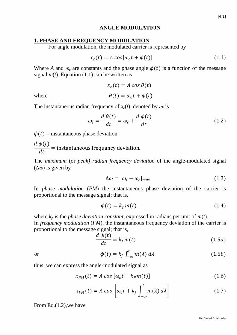
Thus, in PM, the instantaneous frequency 𝜔𝜔𝑖𝑖 varies linearly with the derivative of the modulating signal, and in FM, 𝜔𝜔𝑖𝑖 varies linearly with the modulating signal. Figure (1.1) illustrates AM, FM, and PM waveforms produced by a sinusoidal message waveform.

Fig.(1.1)

U2. FOURIER SPECTRA OF ANGLE-MODULATED SIGNALS An angle-modulated carrier can be represented in exponential form by writing Eq.(1.1) as

𝑥𝑥𝑐𝑐(𝑡𝑡) = 𝑅𝑅𝑅𝑅�𝐴𝐴 𝑅𝑅𝑗𝑗�𝜔𝜔𝑐𝑐𝑡𝑡+𝜙𝜙(𝑡𝑡)�� = 𝑅𝑅𝑅𝑅�𝐴𝐴 𝑅𝑅𝑗𝑗𝜔𝜔𝑐𝑐𝑡𝑡𝑅𝑅𝑗𝑗𝜙𝜙 (𝑡𝑡)� (2.1) Expanding 𝑅𝑅𝑗𝑗𝜙𝜙 (𝑡𝑡)in a power series yields 𝑥𝑥𝑐𝑐(𝑡𝑡) = 𝑅𝑅𝑅𝑅 �𝐴𝐴𝑅𝑅𝑗𝑗𝜔𝜔𝑐𝑐𝑡𝑡 �1 + 𝑗𝑗𝜙𝜙(𝑡𝑡) − 𝜙𝜙2(𝑡𝑡)

2!−⋯+ 𝑗𝑗𝑛𝑛 𝜙𝜙𝑛𝑛 (𝑡𝑡)

𝑛𝑛 !+ ⋯��

= 𝐴𝐴 �𝑐𝑐𝑐𝑐𝑐𝑐 𝜔𝜔𝑐𝑐𝑡𝑡 − 𝜙𝜙(𝑡𝑡)𝑐𝑐𝑖𝑖𝑛𝑛𝜔𝜔𝑐𝑐𝑡𝑡 −𝜙𝜙2(𝑡𝑡)

2! 𝑐𝑐𝑐𝑐𝑐𝑐𝜔𝜔𝑐𝑐𝑡𝑡 +𝜙𝜙3(𝑡𝑡)

3! 𝑐𝑐𝑖𝑖𝑛𝑛𝜔𝜔𝑐𝑐𝑡𝑡 + ⋯� (2.2)

Thus the angle-modulated signal consists of an unmodulated carrier plus various amplitude-modulated terms, such as 𝜙𝜙(𝑡𝑡)𝑐𝑐𝑖𝑖𝑛𝑛 ω𝑐𝑐𝑡𝑡, 𝜙𝜙2(𝑡𝑡)𝑐𝑐𝑐𝑐𝑐𝑐 ω𝑐𝑐𝑡𝑡 , 𝜙𝜙3(𝑡𝑡)𝑐𝑐𝑖𝑖𝑛𝑛 ω𝑐𝑐𝑡𝑡 ... , etc. Hence its Fourier spectrum consists of an unmodulated carrier plus spectra of 𝜙𝜙(𝑡𝑡), 𝜙𝜙2(𝑡𝑡), 𝜙𝜙3(𝑡𝑡),... , etc., centered at ωc. It is clear that the Fourier spectrum of an angle-modulated signal is not related to the message signal spectrum in any simple way, as was the case in AM.

[4.3]


U3. NARROWBAND ANGLE MODULATION If |𝜙𝜙(𝑡𝑡)|𝑚𝑚𝑚𝑚𝑥𝑥 ≪ 1, then Eq. (2.2) can be approximated by [neglecting all higher-power terms of 𝜙𝜙(𝑡𝑡)]

𝑥𝑥𝑐𝑐(𝑡𝑡) ≈ 𝐴𝐴𝑐𝑐𝑐𝑐𝑐𝑐𝜔𝜔𝑐𝑐𝑡𝑡 − 𝐴𝐴𝜙𝜙(𝑡𝑡)𝑐𝑐𝑖𝑖𝑛𝑛𝜔𝜔𝑐𝑐𝑡𝑡 (3.1) 𝑥𝑥𝑐𝑐(𝑡𝑡) in Eq.(3.1) is called the narrowband (NB) angle-modulated signal. Thus,

𝑥𝑥𝑁𝑁𝑁𝑁𝑃𝑃𝑃𝑃 (𝑡𝑡) ≈ 𝐴𝐴𝑐𝑐𝑐𝑐𝑐𝑐𝜔𝜔𝑐𝑐𝑡𝑡 − 𝐴𝐴𝑘𝑘𝑝𝑝 𝑚𝑚(𝑡𝑡)𝑐𝑐𝑖𝑖𝑛𝑛𝜔𝜔𝑐𝑐𝑡𝑡 (3.2)

𝑥𝑥𝑁𝑁𝑁𝑁𝐹𝐹𝑃𝑃 (𝑡𝑡) ≈ 𝐴𝐴𝑐𝑐𝑐𝑐𝑐𝑐𝜔𝜔𝑐𝑐𝑡𝑡 − 𝐴𝐴 �𝑘𝑘𝑓𝑓 � 𝑚𝑚(𝜆𝜆) 𝑑𝑑𝜆𝜆𝑡𝑡

−∞� 𝑐𝑐𝑖𝑖𝑛𝑛𝜔𝜔𝑐𝑐𝑡𝑡 (3.3)

Equation (3.1) indicates that a narrowband angle-modulated signal contains an unmodulated carrier plus a term in which 𝜙𝜙(𝑡𝑡) [a function of m(t)] multiplies a π/2 (rad) phase-shifted carrier. This multiplication generates a pair of sidebands, and if 𝜙𝜙(𝑡𝑡) has a-bandwidth WB, the bandwidth of an NB angle-modulated signal is 2WB. U4. SINUSOIDAL (OR TONE), MODULATION If the message signal m(t) is a pure sinusoid, that is,

𝑚𝑚(𝑡𝑡) = �𝑚𝑚𝑚𝑚𝑐𝑐𝑖𝑖𝑛𝑛𝜔𝜔𝑚𝑚𝑡𝑡 𝑓𝑓𝑐𝑐𝑓𝑓 𝑃𝑃𝑃𝑃𝑚𝑚𝑚𝑚𝑐𝑐𝑐𝑐𝑐𝑐𝜔𝜔𝑚𝑚𝑡𝑡 𝑓𝑓𝑐𝑐𝑓𝑓 𝐹𝐹𝑃𝑃

�

then Eqs. (1.4) and (1.5b) both give 𝜙𝜙(𝑡𝑡) = 𝛽𝛽 𝑐𝑐𝑖𝑖𝑛𝑛𝜔𝜔𝑚𝑚𝑡𝑡 (4.1)

Where

𝛽𝛽 = �𝑘𝑘𝑝𝑝𝑚𝑚𝑚𝑚 𝑓𝑓𝑐𝑐𝑓𝑓 𝑃𝑃𝑃𝑃𝑘𝑘𝑓𝑓𝑚𝑚𝑚𝑚𝜔𝜔𝑚𝑚

𝑓𝑓𝑐𝑐𝑓𝑓 𝐹𝐹𝑃𝑃� (4.2)

The parameter β is known as the Umodulation indexU for angle modulation and is the maximum value of phase deviation for both PM and FM. Note that β is defined only for sinusoidal modulation and it can be expressed as

𝛽𝛽 =Δ𝜔𝜔𝜔𝜔𝑚𝑚

(4.3)

Substituting Eq. (4.1) into Eq. (1.1), we obtain 𝑥𝑥𝑐𝑐(𝑡𝑡) = 𝐴𝐴 𝑐𝑐𝑐𝑐𝑐𝑐[𝜔𝜔𝑐𝑐𝑡𝑡 + 𝛽𝛽 𝑐𝑐𝑖𝑖𝑛𝑛𝜔𝜔𝑚𝑚𝑡𝑡] (4.4)

which can be expressed as 𝑥𝑥𝑐𝑐(𝑡𝑡) = 𝐴𝐴 𝑅𝑅𝑅𝑅(𝑅𝑅𝑗𝑗𝜔𝜔𝑐𝑐𝑡𝑡𝑅𝑅𝑗𝑗𝛽𝛽𝑐𝑐𝑖𝑖𝑛𝑛 𝜔𝜔𝑚𝑚 𝑡𝑡) (4.5)

The function 𝑅𝑅𝑗𝑗𝛽𝛽𝑐𝑐𝑖𝑖𝑛𝑛 𝜔𝜔𝑚𝑚 𝑡𝑡 is clearly a periodic function with period 𝑇𝑇𝑚𝑚 = 2𝜋𝜋 𝜔𝜔𝑚𝑚⁄ . It therefore has a Fourier series representation

𝑅𝑅𝑗𝑗𝛽𝛽𝑐𝑐𝑖𝑖𝑛𝑛 𝜔𝜔𝑚𝑚 𝑡𝑡 = � 𝑐𝑐𝑛𝑛𝑅𝑅𝑗𝑗𝑛𝑛 𝜔𝜔𝑚𝑚 𝑡𝑡∞

𝑛𝑛=−∞

The Fourier coefficients cn can be found to be

𝑐𝑐𝑛𝑛 =𝜔𝜔𝑚𝑚2𝜋𝜋 � 𝑅𝑅𝑗𝑗𝛽𝛽𝑐𝑐𝑖𝑖𝑛𝑛 𝜔𝜔𝑚𝑚 𝑡𝑡

𝜋𝜋 𝜔𝜔𝑚𝑚⁄

−𝜋𝜋 𝜔𝜔𝑚𝑚⁄𝑅𝑅−𝑗𝑗𝑛𝑛 𝜔𝜔𝑚𝑚 𝑡𝑡𝑑𝑑𝑡𝑡

Setting 𝜔𝜔𝑚𝑚𝑡𝑡 = 𝑥𝑥, we have

[4.4]


𝑐𝑐𝑛𝑛 =1

2𝜋𝜋� 𝑅𝑅𝑗𝑗 (𝛽𝛽𝑐𝑐𝑖𝑖𝑛𝑛𝑥𝑥 −𝑛𝑛𝑥𝑥 )𝜋𝜋

−𝜋𝜋𝑑𝑑𝑥𝑥 = 𝐽𝐽𝑛𝑛(𝛽𝛽)

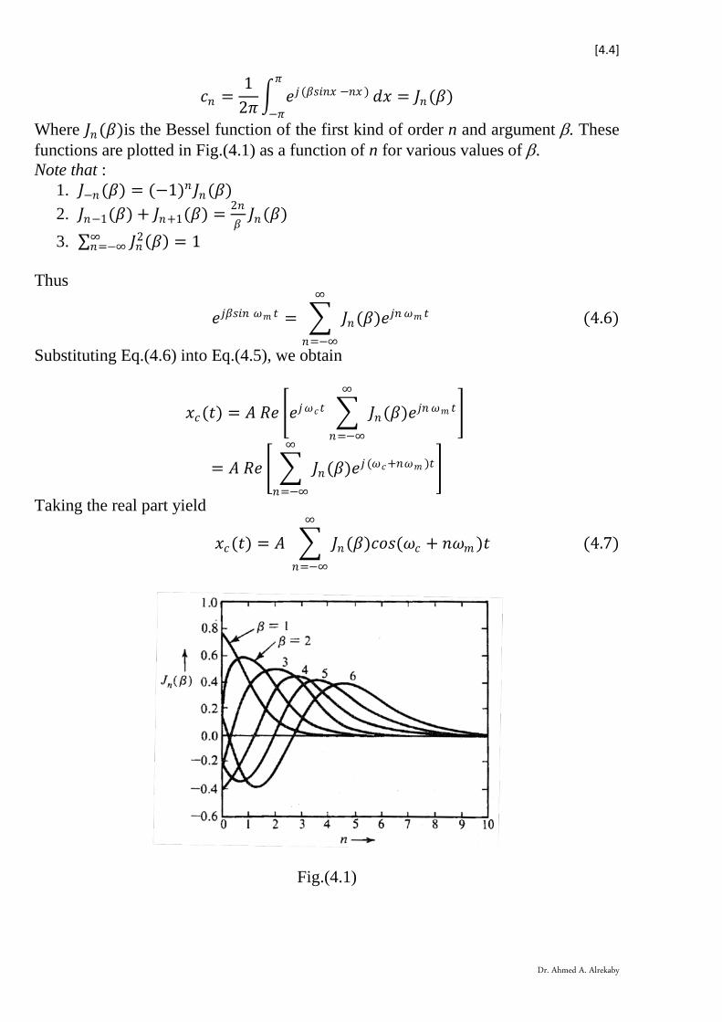
Where 𝐽𝐽𝑛𝑛(𝛽𝛽)is the Bessel function of the first kind of order n and argument β. These functions are plotted in Fig.(4.1) as a function of n for various values of β. Note that :

1. 𝐽𝐽−𝑛𝑛(𝛽𝛽) = (−1)𝑛𝑛𝐽𝐽𝑛𝑛(𝛽𝛽) 2. 𝐽𝐽𝑛𝑛−1(𝛽𝛽) + 𝐽𝐽𝑛𝑛+1(𝛽𝛽) = 2𝑛𝑛

𝛽𝛽𝐽𝐽𝑛𝑛(𝛽𝛽)

3. ∑ 𝐽𝐽𝑛𝑛2(𝛽𝛽) = 1∞𝑛𝑛=−∞

Thus

𝑅𝑅𝑗𝑗𝛽𝛽𝑐𝑐𝑖𝑖𝑛𝑛 𝜔𝜔𝑚𝑚 𝑡𝑡 = � 𝐽𝐽𝑛𝑛(𝛽𝛽)𝑅𝑅𝑗𝑗𝑛𝑛 𝜔𝜔𝑚𝑚 𝑡𝑡∞

𝑛𝑛=−∞

(4.6)

Substituting Eq.(4.6) into Eq.(4.5), we obtain

𝑥𝑥𝑐𝑐(𝑡𝑡) = 𝐴𝐴 𝑅𝑅𝑅𝑅 �𝑅𝑅𝑗𝑗𝜔𝜔𝑐𝑐𝑡𝑡 � 𝐽𝐽𝑛𝑛(𝛽𝛽)𝑅𝑅𝑗𝑗𝑛𝑛𝜔𝜔𝑚𝑚 𝑡𝑡∞

𝑛𝑛=−∞

�

= 𝐴𝐴 𝑅𝑅𝑅𝑅 � � 𝐽𝐽𝑛𝑛(𝛽𝛽)𝑅𝑅𝑗𝑗 (𝜔𝜔𝑐𝑐+𝑛𝑛𝜔𝜔𝑚𝑚 )𝑡𝑡∞

𝑛𝑛=−∞

�

Taking the real part yield

𝑥𝑥𝑐𝑐(𝑡𝑡) = 𝐴𝐴 � 𝐽𝐽𝑛𝑛(𝛽𝛽)𝑐𝑐𝑐𝑐𝑐𝑐(𝜔𝜔𝑐𝑐 + 𝑛𝑛𝜔𝜔𝑚𝑚 )𝑡𝑡∞

𝑛𝑛=−∞

(4.7)

Fig.(4.1)

[4.5]


We observe that; 1. The spectrum consists of a carrier-frequency component plus an infinite number of

sideband components at frequencies ωc ± nωm (n = 1, 2, 3, ... ). 2. The relative amplitudes of the spectral lines depend on the value of Jn(β), and the

value of Jn(β) becomes very small for large values of n. 3. The number of significant spectral lines (that is, having appreciable relative

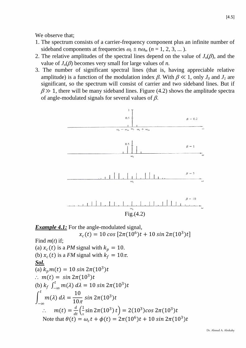
amplitude) is a function of the modulation index β. With β ≪ 1, only J0 and J1 are significant, so the spectrum will consist of carrier and two sideband lines. But if β ≫ 1, there will be many sideband lines. Figure (4.2) shows the amplitude spectra of angle-modulated signals for several values of β.

Fig.(4.2)

UExample 4.1:U For the angle-modulated signal,

𝑥𝑥𝑐𝑐(𝑡𝑡) = 10 𝑐𝑐𝑐𝑐𝑐𝑐 [2𝜋𝜋(106)𝑡𝑡 + 10 𝑐𝑐𝑖𝑖𝑛𝑛 2𝜋𝜋(103)𝑡𝑡] Find m(t) if; (a) 𝑥𝑥𝑐𝑐(𝑡𝑡) is a PM signal with 𝑘𝑘𝑝𝑝 = 10. (b) 𝑥𝑥𝑐𝑐(𝑡𝑡) is a FM signal with 𝑘𝑘𝑓𝑓 = 10π. USol. (a) 𝑘𝑘𝑝𝑝𝑚𝑚(𝑡𝑡) = 10 𝑐𝑐𝑖𝑖𝑛𝑛 2𝜋𝜋(103)𝑡𝑡 ∴ 𝑚𝑚(𝑡𝑡) = 𝑐𝑐𝑖𝑖𝑛𝑛 2𝜋𝜋(103)𝑡𝑡 (b) 𝑘𝑘𝑓𝑓 ∫ 𝑚𝑚(𝜆𝜆) 𝑑𝑑𝜆𝜆𝑡𝑡

−∞ = 10 𝑐𝑐𝑖𝑖𝑛𝑛 2𝜋𝜋(103)𝑡𝑡

� 𝑚𝑚(𝜆𝜆) 𝑑𝑑𝜆𝜆𝑡𝑡

−∞=

1010π 𝑐𝑐𝑖𝑖𝑛𝑛 2𝜋𝜋(103)𝑡𝑡

∴ 𝑚𝑚(𝑡𝑡) = 𝑑𝑑𝑑𝑑𝑡𝑡�1π

sin 2𝜋𝜋(103) 𝑡𝑡� = 2(103)𝑐𝑐𝑐𝑐𝑐𝑐 2𝜋𝜋(103)𝑡𝑡 Note that 𝜃𝜃(𝑡𝑡) = 𝜔𝜔𝑐𝑐𝑡𝑡 + 𝜙𝜙(𝑡𝑡) = 2𝜋𝜋(106)𝑡𝑡 + 10 𝑐𝑐𝑖𝑖𝑛𝑛 2𝜋𝜋(103)𝑡𝑡

[4.6]


and 𝜙𝜙(𝑡𝑡) = 10 𝑐𝑐𝑖𝑖𝑛𝑛 2𝜋𝜋(103)𝑡𝑡 now �́�𝜙(𝑡𝑡) = 20 (𝜋𝜋103) 𝑐𝑐𝑐𝑐𝑐𝑐 2𝜋𝜋(103)𝑡𝑡 thus, the maximum phase deviation is |𝜙𝜙(𝑡𝑡)|𝑚𝑚𝑚𝑚𝑥𝑥 = 10 𝑓𝑓𝑚𝑚𝑑𝑑 And the maximum frequency deviation is Δ𝜔𝜔 = ��́�𝜙(𝑡𝑡)�𝑚𝑚𝑚𝑚𝑥𝑥 = 20 (𝜋𝜋103) 𝑓𝑓𝑚𝑚𝑑𝑑/𝑐𝑐 = 10 𝐾𝐾𝐾𝐾𝐾𝐾 U5. BANDWIDTH OF ANGLE MODULATED SIGNALS U5.1 Sinusoidal Modulation The bandwidth of angle-modulated signal with sinusoidal modulation depends on β and ωm. From mathematic relations;

� 𝐽𝐽𝑛𝑛2(𝛽𝛽) = 𝐽𝐽02(𝛽𝛽) + 2(𝐽𝐽12(𝛽𝛽) + 𝐽𝐽22(𝛽𝛽) + ⋯ ) = 1∞

𝑛𝑛=−∞

This property will help us to find the power of angle modulated signal as 𝑃𝑃 = �𝐴𝐴 𝐽𝐽0(𝛽𝛽) √2⁄ �

2+ 2 ��𝐴𝐴 𝐽𝐽1(𝛽𝛽) √2⁄ �

2+ �𝐴𝐴 𝐽𝐽2(𝛽𝛽) √2⁄ �

2+ ⋯�

=𝐴𝐴2

2[𝐽𝐽02(𝛽𝛽) + 2(𝐽𝐽12(𝛽𝛽) + 𝐽𝐽22(𝛽𝛽) + ⋯ )] =

𝐴𝐴2

2 × 1 =𝐴𝐴2

2 Now we can define the bandwidth of angle modulated signal as the band of frequencies or harmonics which consists about of 98% of the normalized total signal power and is given by;

𝑊𝑊𝑁𝑁 ≈ 2(𝛽𝛽 + 1)𝜔𝜔𝑚𝑚 (5.1) When β ≪ 1, the signal is an NB angle-modulated signal and its bandwidth is approximately equal 2ωm. Usually a value of β < 0.2 is taken to be sufficient to satisfy this condition. Let us consider β =1, then 𝐽𝐽0(1) = 0.7652, 𝐽𝐽1(1) = 0.44, 𝐽𝐽2(1) = 0.1149, 𝐽𝐽3(1) = 0.002477, then the power considered in the terms of n = 0,1, and 2 𝑃𝑃 = 1

2�𝐽𝐽02(1) + 2 �𝐽𝐽12(1) + 𝐽𝐽22(1)��

= 12

[0.76522 + 2(0.442 + 0.11492)] = 0.495 The sum of P for n=2 is 99% of the total power, which is 0.5. If the amplitude 𝐽𝐽𝑛𝑛(𝛽𝛽) < 0.1, it can be neglected. U5.2 Arbitrary Modulation: For an angle-modulated signal with an arbitrary modulating signal m(t) band-limited to ωM rad/s, we define the deviation ratio D as

𝐷𝐷 =𝑚𝑚𝑚𝑚𝑥𝑥𝑖𝑖𝑚𝑚𝑚𝑚𝑚𝑚 𝑓𝑓𝑓𝑓𝑅𝑅𝑓𝑓𝑚𝑚𝑅𝑅𝑛𝑛𝑐𝑐𝑓𝑓 𝑑𝑑𝑅𝑅𝑑𝑑𝑖𝑖𝑚𝑚𝑡𝑡𝑖𝑖𝑐𝑐𝑛𝑛

𝑏𝑏𝑚𝑚𝑛𝑛𝑑𝑑𝑏𝑏𝑖𝑖𝑑𝑑𝑡𝑡ℎ 𝑐𝑐𝑓𝑓 𝑚𝑚(𝑡𝑡) =∆𝜔𝜔𝜔𝜔𝑃𝑃

(5.2)

The deviation ratio D plays the same role for arbitrary modulation as the modulation index β plays for sinusoidal modulation. Replacing β by D and ωm by ωM in Eq. (5.1), we have

𝑊𝑊𝑁𝑁 ≈ 2(𝐷𝐷 + 1)𝜔𝜔𝑃𝑃 ≈ 2(∆𝜔𝜔 + 𝜔𝜔𝑃𝑃) (5.3)

[4.7]


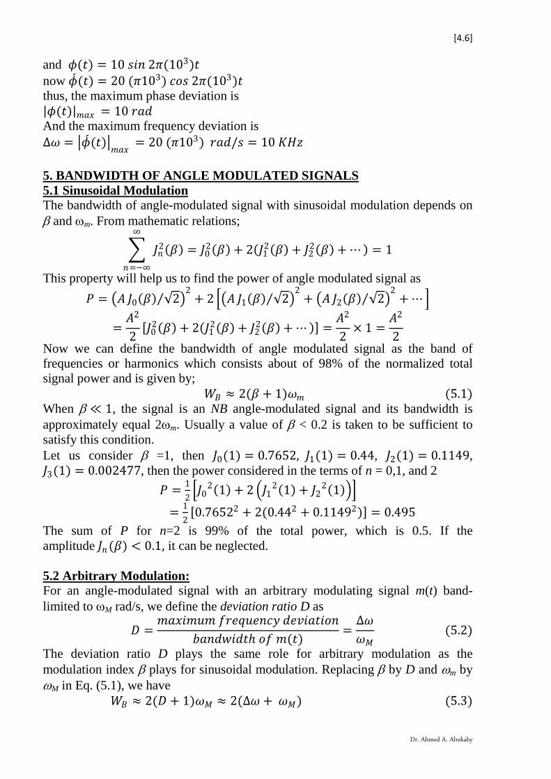
This expression for bandwidth is generally referred to as Carson's rule. If 𝐷𝐷 ≪ 1, the bandwidth is approximately 2ωM ,and the signal is known as a narrowband (NB) angle-modulated signal. If 𝐷𝐷 ≫ 1, the bandwidth is approximately 2DωM = 2∆ω, which is twice the peak frequency deviation. Such a signal is called a wideband (WB) angle-modulated signal. UExample 5.1: (a) Estimate BFM and BPM for the modulating signal m(t) for kf = 2π×105 and kp = 5π . (b) Repeat the problem if the amplitude of m(t) is doubled.

USol. (a) The peak amplitude of m(t) is unity. Hence, �𝑚𝑚(𝑡𝑡)|𝑚𝑚𝑚𝑚𝑥𝑥 = 1. We now determine the essential bandwidth B of m(t). The Fourier series for this periodic signal is given by

𝑚𝑚(𝑡𝑡) = �𝑚𝑚𝑛𝑛𝑐𝑐𝑐𝑐𝑐𝑐 𝑛𝑛𝜔𝜔𝑐𝑐𝑡𝑡 𝜔𝜔𝑐𝑐 =2𝜋𝜋

2 × 10−4 = 104𝜋𝜋𝑛𝑛

Where

𝑚𝑚𝑛𝑛 = �−8𝜋𝜋2𝑛𝑛2 𝑛𝑛 𝑐𝑐𝑑𝑑𝑑𝑑0 𝑛𝑛 𝑅𝑅𝑑𝑑𝑅𝑅𝑛𝑛

�

It can be seen that the harmonic amplitudes decrease rapidly with n. The third and fifth harmonic powers are 1.21 and 0.16%, respectively, of the fundamental component power. Hence, we are justified in assuming the essential bandwidth of m(t) as the frequency of the third harmonic, that is, 3(104/2) Hz. Thus,

fM =15 kHz UFor FM:

∆𝑓𝑓 =∆𝜔𝜔2𝜋𝜋 =

12𝜋𝜋 𝑘𝑘𝑓𝑓

�𝑚𝑚(𝑡𝑡)|𝑚𝑚𝑚𝑚𝑥𝑥 =1

2𝜋𝜋 (2π × 105) × 1 = 100 𝑘𝑘𝐾𝐾𝐾𝐾 and

𝑁𝑁𝐹𝐹𝑃𝑃 = 2(∆𝑓𝑓 + 𝑓𝑓𝑃𝑃) = 230 𝑘𝑘𝐾𝐾𝐾𝐾 The deviation ratio D is given by

𝐷𝐷 =∆𝑓𝑓𝑓𝑓𝑃𝑃

=10015

UFor PM:U the peak amplitude of �́�𝑚(𝑡𝑡) is 2×104 and

∆𝑓𝑓 =1

2𝜋𝜋 𝑘𝑘𝑝𝑝��́�𝑚(𝑡𝑡)|𝑚𝑚𝑚𝑚𝑥𝑥 = 50 𝑘𝑘𝐾𝐾𝐾𝐾

Hence, 𝑁𝑁𝑃𝑃𝑃𝑃 = 2(∆𝑓𝑓 + 𝑓𝑓𝑃𝑃) = 130 𝑘𝑘𝐾𝐾𝐾𝐾

and

[4.8]



=5015

(b) Doubling m(t) doubles its peak value. Hence, �𝑚𝑚(𝑡𝑡)|𝑚𝑚𝑚𝑚𝑥𝑥 =2. But its bandwidth is unchanged (𝑓𝑓𝑃𝑃 = 15 𝑘𝑘𝐾𝐾𝐾𝐾). UFor FM:

∆𝑓𝑓 =1

2𝜋𝜋 𝑘𝑘𝑓𝑓�𝑚𝑚(𝑡𝑡)|𝑚𝑚𝑚𝑚𝑥𝑥 =

12𝜋𝜋 (2π × 105) × 2 = 200 𝑘𝑘𝐾𝐾𝐾𝐾

and 𝑁𝑁𝐹𝐹𝑃𝑃 = 2(∆𝑓𝑓 + 𝑓𝑓𝑃𝑃) = 430 𝑘𝑘𝐾𝐾𝐾𝐾

The deviation ratio D is given by


=20015

UFor PM:U Doubling m(t) doubles its derivative so that now ��́�𝑚(𝑡𝑡)|𝑚𝑚𝑚𝑚𝑥𝑥 = 4×104, and

∆𝑓𝑓 =1

2𝜋𝜋 𝑘𝑘𝑝𝑝��́�𝑚(𝑡𝑡)|𝑚𝑚𝑚𝑚𝑥𝑥 = 100𝑘𝑘𝐾𝐾𝐾𝐾


and


=10015

Observe that doubling the signal amplitude roughly doubles the bandwidth of both FM and PM waveforms. If m(t) is time-expanded by a factor of 2; that is, if the period of m(t) is 4×10-4 ,then the signal spectral width (bandwidth) reduces by a factor of 2. We can verify this by observing that the fundamental frequency is now 2.5 kHz, and its third harmonic is 7.5 kHz. Hence, fM = 7.5 kHz, which is half the previous bandwidth. Moreover, time expansion does not affect the peak amplitude so that �𝑚𝑚(𝑡𝑡)|𝑚𝑚𝑚𝑚𝑥𝑥 = 1. However, ��́�𝑚(𝑡𝑡)|𝑚𝑚𝑚𝑚𝑥𝑥 is halved, that is, ��́�𝑚(𝑡𝑡)|𝑚𝑚𝑚𝑚𝑥𝑥 = 10, 000. UFor FM:

∆𝑓𝑓 =1

2𝜋𝜋 𝑘𝑘𝑓𝑓�𝑚𝑚(𝑡𝑡)|𝑚𝑚𝑚𝑚𝑥𝑥 = 100 𝑘𝑘𝐾𝐾𝐾𝐾

and 𝑁𝑁𝐹𝐹𝑃𝑃 = 2(∆𝑓𝑓 + 𝑓𝑓𝑃𝑃) = 2(100 + 7.5) = 215 𝑘𝑘𝐾𝐾𝐾𝐾

UFor PM:

∆𝑓𝑓 =1

2𝜋𝜋 𝑘𝑘𝑝𝑝��́�𝑚(𝑡𝑡)|𝑚𝑚𝑚𝑚𝑥𝑥 = 25 𝑘𝑘𝐾𝐾𝐾𝐾


[4.9]


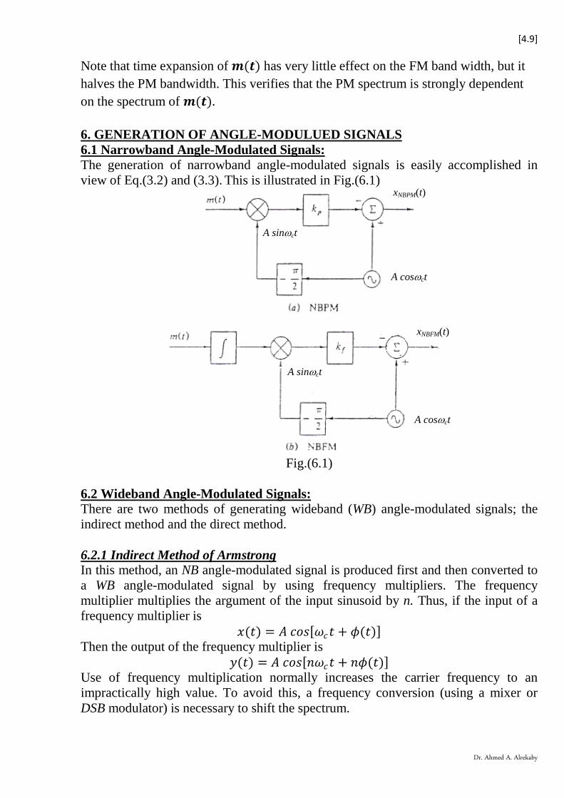
Note that time expansion of 𝒎𝒎(𝒕𝒕) has very little effect on the FM band width, but it halves the PM bandwidth. This verifies that the PM spectrum is strongly dependent on the spectrum of 𝒎𝒎(𝒕𝒕). U6. GENERATION OF ANGLE-MODULUED SIGNALS U6.1 Narrowband Angle-Modulated Signals: The generation of narrowband angle-modulated signals is easily accomplished in view of Eq.(3.2) and (3.3). This is illustrated in Fig.(6.1)

Fig.(6.1)

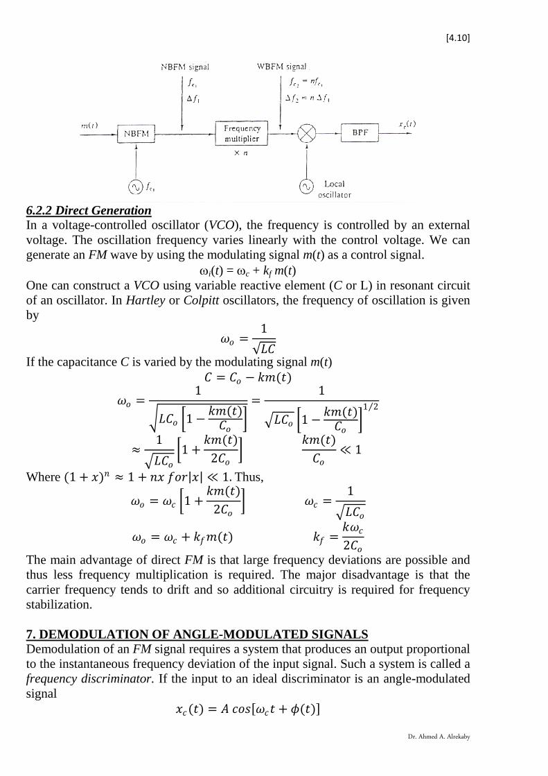
U6.2 Wideband Angle-Modulated Signals: There are two methods of generating wideband (WB) angle-modulated signals; the indirect method and the direct method. U6.2.1 Indirect Method of Armstrong In this method, an NB angle-modulated signal is produced first and then converted to a WB angle-modulated signal by using frequency multipliers. The frequency multiplier multiplies the argument of the input sinusoid by n. Thus, if the input of a frequency multiplier is

𝑥𝑥(𝑡𝑡) = 𝐴𝐴 𝑐𝑐𝑐𝑐𝑐𝑐[𝜔𝜔𝑐𝑐𝑡𝑡 + 𝜙𝜙(𝑡𝑡)] Then the output of the frequency multiplier is

𝑓𝑓(𝑡𝑡) = 𝐴𝐴 𝑐𝑐𝑐𝑐𝑐𝑐[𝑛𝑛𝜔𝜔𝑐𝑐𝑡𝑡 + 𝑛𝑛𝜙𝜙(𝑡𝑡)] Use of frequency multiplication normally increases the carrier frequency to an impractically high value. To avoid this, a frequency conversion (using a mixer or DSB modulator) is necessary to shift the spectrum.

xNBFM(t)

xNBPM(t)

A cosωct

A sinωct

A sinωct

A cosωct

[4.10]


U6.2.2 Direct Generation In a voltage-controlled oscillator (VCO), the frequency is controlled by an external voltage. The oscillation frequency varies linearly with the control voltage. We can generate an FM wave by using the modulating signal m(t) as a control signal.

ωi(t) = ωc + kf m(t) One can construct a VCO using variable reactive element (C or L) in resonant circuit of an oscillator. In Hartley or Colpitt oscillators, the frequency of oscillation is given by

𝜔𝜔𝑐𝑐 =1

√𝐿𝐿𝐿𝐿

If the capacitance C is varied by the modulating signal m(t) 𝐿𝐿 = 𝐿𝐿𝑐𝑐 − 𝑘𝑘𝑚𝑚(𝑡𝑡)

𝜔𝜔𝑐𝑐 =1

�𝐿𝐿𝐿𝐿𝑐𝑐 �1 −𝑘𝑘𝑚𝑚(𝑡𝑡)𝐿𝐿𝑐𝑐

�=

1

�𝐿𝐿𝐿𝐿𝑐𝑐 �1 −𝑘𝑘𝑚𝑚(𝑡𝑡)𝐿𝐿𝑐𝑐

�1 2⁄

≈1

�𝐿𝐿𝐿𝐿𝑐𝑐�1 +

𝑘𝑘𝑚𝑚(𝑡𝑡)2𝐿𝐿𝑐𝑐

� 𝑘𝑘𝑚𝑚(𝑡𝑡)𝐿𝐿𝑐𝑐

≪ 1

Where (1 + 𝑥𝑥)𝑛𝑛 ≈ 1 + 𝑛𝑛𝑥𝑥 𝑓𝑓𝑐𝑐𝑓𝑓|𝑥𝑥| ≪ 1. Thus,

𝜔𝜔𝑐𝑐 = 𝜔𝜔𝑐𝑐 �1 +𝑘𝑘𝑚𝑚(𝑡𝑡)

2𝐿𝐿𝑐𝑐� 𝜔𝜔𝑐𝑐 =

1�𝐿𝐿𝐿𝐿𝑐𝑐

𝜔𝜔𝑐𝑐 = 𝜔𝜔𝑐𝑐 + 𝑘𝑘𝑓𝑓𝑚𝑚(𝑡𝑡) 𝑘𝑘𝑓𝑓 =𝑘𝑘𝜔𝜔𝑐𝑐2𝐿𝐿𝑐𝑐

The main advantage of direct FM is that large frequency deviations are possible and thus less frequency multiplication is required. The major disadvantage is that the carrier frequency tends to drift and so additional circuitry is required for frequency stabilization. U7. DEMODULATION OF ANGLE-MODULATED SIGNALS Demodulation of an FM signal requires a system that produces an output proportional to the instantaneous frequency deviation of the input signal. Such a system is called a frequency discriminator. If the input to an ideal discriminator is an angle-modulated signal

𝑥𝑥𝑐𝑐(𝑡𝑡) = 𝐴𝐴 𝑐𝑐𝑐𝑐𝑐𝑐[𝜔𝜔𝑐𝑐𝑡𝑡 + 𝜙𝜙(𝑡𝑡)]

[4.11]


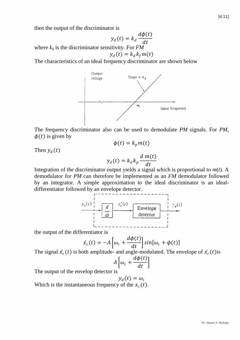
then the output of the discriminator is

𝑓𝑓𝑑𝑑(𝑡𝑡) = 𝑘𝑘𝑑𝑑𝑑𝑑𝜙𝜙(𝑡𝑡)𝑑𝑑𝑡𝑡

where kd is the discriminator sensitivity. For FM 𝑓𝑓𝑑𝑑(𝑡𝑡) = 𝑘𝑘𝑑𝑑𝑘𝑘𝑓𝑓𝑚𝑚(𝑡𝑡)

The characteristics of an ideal frequency discriminator are shown below

The frequency discriminator also can be used to demodulate PM signals. For PM, 𝜙𝜙(𝑡𝑡) is given by

𝜙𝜙(𝑡𝑡) = 𝑘𝑘𝑝𝑝𝑚𝑚(𝑡𝑡) Then 𝑓𝑓𝑑𝑑(𝑡𝑡)

𝑓𝑓𝑑𝑑(𝑡𝑡) = 𝑘𝑘𝑑𝑑𝑘𝑘𝑝𝑝𝑑𝑑 𝑚𝑚(𝑡𝑡)𝑑𝑑𝑡𝑡

Integration of the discriminator output yields a signal which is proportional to m(t). A demodulator for PM can therefore be implemented as an FM demodulator followed by an integrator. A simple approximation to the ideal discriminator is an ideal- differentiator followed by an envelope detector.

the output of the differentiator is

𝑥𝑥�́�𝑐(𝑡𝑡) = −𝐴𝐴 �𝜔𝜔𝑐𝑐 +𝑑𝑑𝜙𝜙(𝑡𝑡)𝑑𝑑𝑡𝑡 � 𝑐𝑐𝑖𝑖𝑛𝑛[𝜔𝜔𝑐𝑐 + 𝜙𝜙(𝑡𝑡)]

The signal 𝑥𝑥�́�𝑐(𝑡𝑡) is both amplitude- and angle-modulated. The envelope of 𝑥𝑥�́�𝑐(𝑡𝑡)is

𝐴𝐴 �𝜔𝜔𝑐𝑐 +𝑑𝑑𝜙𝜙(𝑡𝑡)𝑑𝑑𝑡𝑡 �

The output of the envelop detector is 𝑓𝑓𝑑𝑑(𝑡𝑡) = 𝜔𝜔𝑖𝑖

Which is the instantaneous frequency of the 𝑥𝑥𝑐𝑐(𝑡𝑡).

[4.12]


U8. NOISE IN ANGLE MODULATION SYSTEMS The transmitted signal 𝑋𝑋𝑐𝑐(𝑡𝑡) has the form

𝑋𝑋𝑐𝑐(𝑡𝑡) = 𝐴𝐴𝑐𝑐 𝑐𝑐𝑐𝑐𝑐𝑐[𝜔𝜔𝑐𝑐𝑡𝑡 + 𝜙𝜙(𝑡𝑡)] (8.1) Where

𝜙𝜙(𝑡𝑡) = �𝑘𝑘𝑝𝑝𝑋𝑋(𝑡𝑡) 𝑓𝑓𝑐𝑐𝑓𝑓 𝑃𝑃𝑃𝑃

𝑘𝑘𝑓𝑓 � 𝑋𝑋(𝜆𝜆) 𝑑𝑑𝜆𝜆 𝑓𝑓𝑐𝑐𝑓𝑓 𝐹𝐹𝑃𝑃𝑡𝑡

−∞

� (8.2)

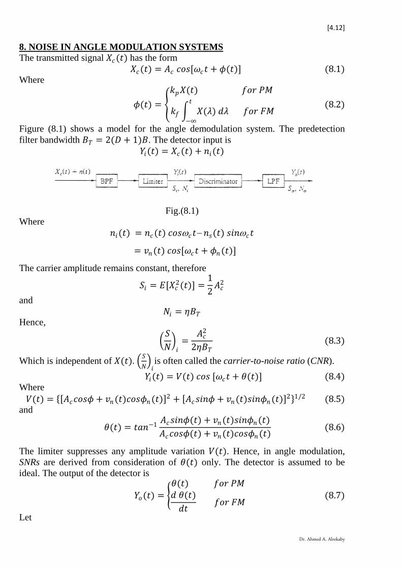
Figure (8.1) shows a model for the angle demodulation system. The predetection filter bandwidth 𝑁𝑁𝑇𝑇 = 2(𝐷𝐷 + 1)𝑁𝑁. The detector input is

𝑌𝑌𝑖𝑖(𝑡𝑡) = 𝑋𝑋𝑐𝑐(𝑡𝑡) + 𝑛𝑛𝑖𝑖(𝑡𝑡)

Fig.(8.1) Where

𝑛𝑛𝑖𝑖(𝑡𝑡) = 𝑛𝑛𝑐𝑐(𝑡𝑡) 𝑐𝑐𝑐𝑐𝑐𝑐ω𝑐𝑐 𝑡𝑡− 𝑛𝑛𝑐𝑐(𝑡𝑡) 𝑐𝑐𝑖𝑖𝑛𝑛ω𝑐𝑐𝑡𝑡

= 𝑑𝑑𝑛𝑛(𝑡𝑡) 𝑐𝑐𝑐𝑐𝑐𝑐[𝜔𝜔𝑐𝑐𝑡𝑡 + 𝜙𝜙𝑛𝑛(𝑡𝑡)]

The carrier amplitude remains constant, therefore

𝑆𝑆𝑖𝑖 = 𝐸𝐸[𝑋𝑋𝑐𝑐2(𝑡𝑡)] =12𝐴𝐴𝑐𝑐

2 and

𝑁𝑁𝑖𝑖 = 𝜂𝜂𝑁𝑁𝑇𝑇 Hence,

�𝑆𝑆𝑁𝑁�𝑖𝑖

=𝐴𝐴𝑐𝑐2

2𝜂𝜂𝑁𝑁𝑇𝑇 (8.3)

Which is independent of 𝑋𝑋(𝑡𝑡). �𝑆𝑆𝑁𝑁�𝑖𝑖is often called the carrier-to-noise ratio (CNR).

𝑌𝑌𝑖𝑖(𝑡𝑡) = 𝑉𝑉(𝑡𝑡) 𝑐𝑐𝑐𝑐𝑐𝑐 [𝜔𝜔𝑐𝑐𝑡𝑡 + 𝜃𝜃(𝑡𝑡)] (8.4) Where 𝑉𝑉(𝑡𝑡) = {[𝐴𝐴𝑐𝑐𝑐𝑐𝑐𝑐𝑐𝑐𝜙𝜙 + 𝑑𝑑𝑛𝑛(𝑡𝑡)𝑐𝑐𝑐𝑐𝑐𝑐𝜙𝜙𝑛𝑛(𝑡𝑡)]2 + [𝐴𝐴𝑐𝑐𝑐𝑐𝑖𝑖𝑛𝑛𝜙𝜙 + 𝑑𝑑𝑛𝑛(𝑡𝑡)𝑐𝑐𝑖𝑖𝑛𝑛𝜙𝜙𝑛𝑛(𝑡𝑡)]2}1/2 (8.5)

and

𝜃𝜃(𝑡𝑡) = 𝑡𝑡𝑚𝑚𝑛𝑛−1 𝐴𝐴𝑐𝑐𝑐𝑐𝑖𝑖𝑛𝑛𝜙𝜙(𝑡𝑡) + 𝑑𝑑𝑛𝑛(𝑡𝑡)𝑐𝑐𝑖𝑖𝑛𝑛𝜙𝜙𝑛𝑛(𝑡𝑡)𝐴𝐴𝑐𝑐𝑐𝑐𝑐𝑐𝑐𝑐𝜙𝜙(𝑡𝑡) + 𝑑𝑑𝑛𝑛(𝑡𝑡)𝑐𝑐𝑐𝑐𝑐𝑐𝜙𝜙𝑛𝑛(𝑡𝑡) (8.6)

The limiter suppresses any amplitude variation 𝑉𝑉(𝑡𝑡). Hence, in angle modulation, SNRs are derived from consideration of 𝜃𝜃(𝑡𝑡) only. The detector is assumed to be ideal. The output of the detector is

𝑌𝑌𝑐𝑐(𝑡𝑡) = �𝜃𝜃(𝑡𝑡) 𝑓𝑓𝑐𝑐𝑓𝑓 𝑃𝑃𝑃𝑃𝑑𝑑 𝜃𝜃(𝑡𝑡)𝑑𝑑𝑡𝑡 𝑓𝑓𝑐𝑐𝑓𝑓 𝐹𝐹𝑃𝑃

(8.7) �

Let

[4.13]


𝑌𝑌𝑖𝑖(𝑡𝑡) = 𝑅𝑅𝑅𝑅�𝑌𝑌(𝑡𝑡)𝑅𝑅𝑗𝑗𝜔𝜔𝑐𝑐𝑡𝑡� (8.8) where

𝑌𝑌(𝑡𝑡) = 𝐴𝐴𝑐𝑐𝑅𝑅𝑗𝑗𝜙𝜙(𝑡𝑡) + 𝑑𝑑𝑛𝑛𝑅𝑅𝑗𝑗𝜙𝜙𝑛𝑛 (𝑡𝑡) (8.9)

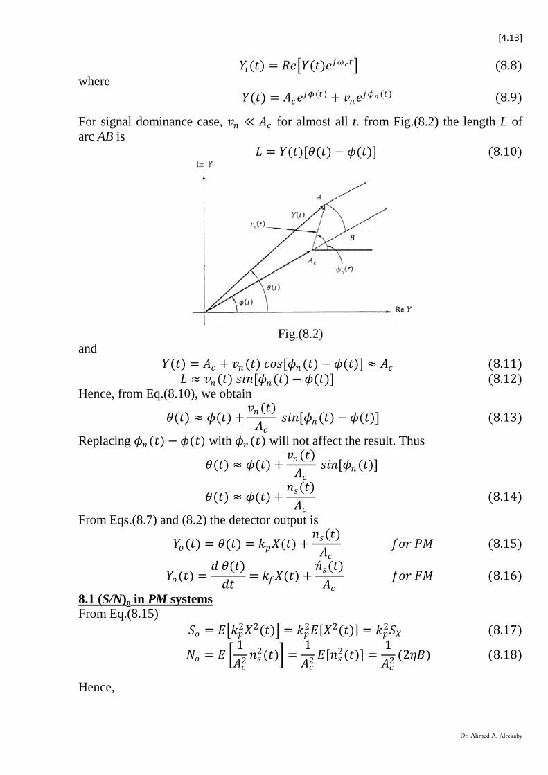
For signal dominance case, 𝑑𝑑𝑛𝑛 ≪ 𝐴𝐴𝑐𝑐 for almost all t. from Fig.(8.2) the length L of arc AB is

𝐿𝐿 = 𝑌𝑌(𝑡𝑡)[𝜃𝜃(𝑡𝑡) − 𝜙𝜙(𝑡𝑡)] (8.10)

Fig.(8.2)

and 𝑌𝑌(𝑡𝑡) = 𝐴𝐴𝑐𝑐 + 𝑑𝑑𝑛𝑛(𝑡𝑡) 𝑐𝑐𝑐𝑐𝑐𝑐[𝜙𝜙𝑛𝑛(𝑡𝑡) − 𝜙𝜙(𝑡𝑡)] ≈ 𝐴𝐴𝑐𝑐 (8.11)

𝐿𝐿 ≈ 𝑑𝑑𝑛𝑛(𝑡𝑡) 𝑐𝑐𝑖𝑖𝑛𝑛[𝜙𝜙𝑛𝑛(𝑡𝑡) − 𝜙𝜙(𝑡𝑡)] (8.12) Hence, from Eq.(8.10), we obtain

𝜃𝜃(𝑡𝑡) ≈ 𝜙𝜙(𝑡𝑡) +𝑑𝑑𝑛𝑛(𝑡𝑡)𝐴𝐴𝑐𝑐

𝑐𝑐𝑖𝑖𝑛𝑛[𝜙𝜙𝑛𝑛(𝑡𝑡) − 𝜙𝜙(𝑡𝑡)] (8.13)

Replacing 𝜙𝜙𝑛𝑛(𝑡𝑡) − 𝜙𝜙(𝑡𝑡) with 𝜙𝜙𝑛𝑛(𝑡𝑡) will not affect the result. Thus

𝜃𝜃(𝑡𝑡) ≈ 𝜙𝜙(𝑡𝑡) +𝑑𝑑𝑛𝑛(𝑡𝑡)𝐴𝐴𝑐𝑐

𝑐𝑐𝑖𝑖𝑛𝑛[𝜙𝜙𝑛𝑛(𝑡𝑡)]

𝜃𝜃(𝑡𝑡) ≈ 𝜙𝜙(𝑡𝑡) +𝑛𝑛𝑐𝑐(𝑡𝑡)𝐴𝐴𝑐𝑐

(8.14)

From Eqs.(8.7) and (8.2) the detector output is

𝑌𝑌𝑐𝑐(𝑡𝑡) = 𝜃𝜃(𝑡𝑡) = 𝑘𝑘𝑝𝑝𝑋𝑋(𝑡𝑡) +𝑛𝑛𝑐𝑐(𝑡𝑡)𝐴𝐴𝑐𝑐

𝑓𝑓𝑐𝑐𝑓𝑓 𝑃𝑃𝑃𝑃 (8.15)

𝑌𝑌𝑐𝑐(𝑡𝑡) =𝑑𝑑 𝜃𝜃(𝑡𝑡)𝑑𝑑𝑡𝑡 = 𝑘𝑘𝑓𝑓𝑋𝑋(𝑡𝑡) +

�́�𝑛𝑐𝑐(𝑡𝑡)𝐴𝐴𝑐𝑐

𝑓𝑓𝑐𝑐𝑓𝑓 𝐹𝐹𝑃𝑃 (8.16)

U8.1 (S/N)o in PM systems From Eq.(8.15)

𝑆𝑆𝑐𝑐 = 𝐸𝐸�𝑘𝑘𝑝𝑝2𝑋𝑋2(𝑡𝑡)� = 𝑘𝑘𝑝𝑝2𝐸𝐸[𝑋𝑋2(𝑡𝑡)] = 𝑘𝑘𝑝𝑝2𝑆𝑆𝑋𝑋 (8.17)

𝑁𝑁𝑐𝑐 = 𝐸𝐸 �1𝐴𝐴𝑐𝑐2

𝑛𝑛𝑐𝑐2(𝑡𝑡)� =1𝐴𝐴𝑐𝑐2

𝐸𝐸[𝑛𝑛𝑐𝑐2(𝑡𝑡)] =1𝐴𝐴𝑐𝑐2

(2𝜂𝜂𝑁𝑁) (8.18)

Hence,

[4.14]


�𝑆𝑆𝑁𝑁�𝑐𝑐

=𝑘𝑘𝑝𝑝2𝐴𝐴𝑐𝑐2𝑆𝑆𝑋𝑋

2𝜂𝜂𝑁𝑁 (8.19)

Since,

𝛾𝛾 =𝑆𝑆𝑖𝑖𝜂𝜂𝑁𝑁 =

𝐴𝐴𝑐𝑐2

2𝜂𝜂𝑁𝑁 (8.20)

Eq.(8.19) can be expressed as


= 𝑘𝑘𝑝𝑝2𝑆𝑆𝑋𝑋𝛾𝛾 (8.21)

U8.2 (S/N)o in FM systems From Eq.(8.16)

𝑆𝑆𝑐𝑐 = 𝐸𝐸�𝑘𝑘𝑓𝑓2𝑋𝑋2(𝑡𝑡)� = 𝑘𝑘𝑓𝑓2𝐸𝐸[𝑋𝑋2(𝑡𝑡)] = 𝑘𝑘𝑓𝑓2𝑆𝑆𝑋𝑋 (8.22)

𝑁𝑁𝑐𝑐 = 𝐸𝐸 �1𝐴𝐴𝑐𝑐2

[�́�𝑛𝑐𝑐(𝑡𝑡)]2� =1𝐴𝐴𝑐𝑐2

𝐸𝐸[[�́�𝑛𝑐𝑐(𝑡𝑡)]2] (8.23)

The PSD of �́�𝑛𝑐𝑐(𝑡𝑡) is given by

𝑆𝑆𝑛𝑛�́�𝑐�́�𝑛𝑐𝑐 (𝜔𝜔) = 𝜔𝜔2𝑆𝑆𝑛𝑛𝑐𝑐𝑛𝑛𝑐𝑐(𝜔𝜔) = �𝜔𝜔2𝜂𝜂 𝑓𝑓𝑐𝑐𝑓𝑓 |𝜔𝜔| < 𝑊𝑊 (= 2𝜋𝜋𝑁𝑁)

0 𝑐𝑐𝑡𝑡ℎ𝑅𝑅𝑓𝑓𝑏𝑏𝑖𝑖𝑐𝑐𝑅𝑅� (8.24)

Then

𝑁𝑁𝑐𝑐 =1𝐴𝐴𝑐𝑐2

12𝜋𝜋� 𝜔𝜔2𝜂𝜂 𝑑𝑑𝜔𝜔 =

23𝜂𝜂𝐴𝐴𝑐𝑐2

𝑊𝑊3

2𝜋𝜋

𝑊𝑊

−𝑊𝑊 (8.25)

Hence,


=3𝐴𝐴𝑐𝑐2(2𝜋𝜋)𝑘𝑘𝑓𝑓2𝑆𝑆𝑋𝑋

2𝜂𝜂𝑊𝑊3 (8.26)

Using Eq.(8.20), we can express Eq.(8.26) as


= 3�𝑘𝑘𝑓𝑓2𝑆𝑆𝑋𝑋𝑊𝑊2 ��

𝐴𝐴𝑐𝑐2

2𝜂𝜂𝑁𝑁�= 3�

𝑘𝑘𝑓𝑓2𝑆𝑆𝑋𝑋𝑊𝑊2 �𝛾𝛾 (8.27)

Since Δ𝜔𝜔 = �𝑘𝑘𝑓𝑓𝑋𝑋(𝑡𝑡)�𝑚𝑚𝑚𝑚𝑥𝑥

= 𝑘𝑘𝑓𝑓[|𝑋𝑋(𝑡𝑡)| ≤ 1], Eq.(8.27) can be rewritten as


= 3 �Δ𝜔𝜔𝑊𝑊 �

2

𝑆𝑆𝑋𝑋𝛾𝛾 = 3𝐷𝐷2𝑆𝑆𝑋𝑋𝛾𝛾 (8.28)

Equation (8.25) indicates that the output noise power is inversely proportional to the mean carrier power �𝐴𝐴𝑐𝑐

2

2� in FM. This effect is called Unoise quietingU.

UExample 8.1:U consider an FM broadcast system with parameter ∆f=75 kHz and B=15 kHz. Assuming 𝑆𝑆𝑋𝑋 = 1

2, find the output SNR and calculate the improvement (in dB) over the baseband system. USol. Substituting the given parameters into Eq.(8.28), we obtain


= 3�75(103)15(103)�

2

�12� 𝛾𝛾 = 37.5𝛾𝛾

Now, 10 log 37.5=15.7 dB, which indicates that (𝑆𝑆/𝑁𝑁)𝑐𝑐 is about 16 dB better than the baseband system.

ANGLE MODULATION - جامعة بابل | University of Babylon maximum (or peak) radian frequency...

Documents

Transcript of ANGLE MODULATION - جامعة بابل | University of Babylon maximum (or peak) radian frequency...