1

Lf

vLreffr

∆−= 22 ε

ο

Analysis Of Feed Point Coordinates Of A Coaxial Feed Rectangular Microstrip Antenna

Using Mlpffbp Artificial Neural Network V. V. Thakare1 & P. K. Singhal2

1 Deptt. of Electronics and Instrumentation , Anand Engineering College, Keetham, Agra, 282007, India. vandanavt_19@rediffmail.com

2 Deptt. of Electronics Engineering ,Madhav Institute of Technology & Science, Near Gola Ka Mandir, Gwalior, 474005, India .

pks_65@yahoo.com Abstract: The present work carries out the comparative evaluation of 6 different variants of back-propagation training algorithm for the determination of feed point coordinates of a coaxial probe feed rectangular microstrip antenna for the given values of resonating frequency and patch dimensions i.e. length and width with constant dielectric constant and substrate height using multilayer feed forward back propagation (MLPFFBP) artificial neural network. A relative performance analysis of the proposed neural network for different training algorithms, number of neurons and number hidden layers is also carried out for estimating the feed point with particular attention paid to the speed of computation and accuracy achieved. A relative performance of the different training algorithms is carried out for estimating the feed point with particular attention paid to the speed of computation and accuracy achieved. The network training data is generated using IE3D an Electromagnetic simulator. Results of the network are compared with the data obtained from IE3D simulator and concluded that results are in good agreement with simulator findings. Keywords: Microstrip antenna, feed point coordinates, feed position, neural network, MLPFFBP, ANN.

I. INTRODUCTION

An accurate physics-based modelling of

microwave circuits is an essential part of now a day’s computer aided microwave circuit design. Electromagnetic simulators deliver the accuracy with the drawback of large computational expenses. Recently, neural networks have been introduced into the microwave engineering community [1-2] as a fast and flexible tool for microwave circuit modelling and design. This paper concentrates on the building of neural networks for microstrip antenna which are the circuits with highly non-linear responses as they have resonant structure [3]. Thus, the networks are built by multi-layer perceptron (MLP) Networks with a relatively optimum number of hidden

neurons to achieve the required degree of freedom and accuracy. In this paper, a multilayer feed-forward back propagation [4] artificial neural network trained by different training algorithms is used to estimate the feed point coordinates of a coaxial probe feed rectangular microstrip antenna for the given values patch dimensions and resonating in the frequency range of 1.7 GHz – 2.5 GHz.

Sufficient amount of work [5-12] indicates how

ANN have been used efficiently to design rectangular microstrip antenna for the determination of different design parameters of rectangular microstrip antenna like patch dimensions i.e. length, width, substrate thickness, dielectric constants, input impedance, radiation efficiency and resonant frequencies of triangular and rectangular microstrip antennas. Based on these considerations, a comparative evaluation of different variants of back-propagation training algorithm is achieved for the determination of exact feed position of rectangular microstrip antenna using artificial neural network (ANN) for maximum bandwidth through this piece of work. However such analysis of microstrip antennas is complicated and exhaustive. To optimize the antenna efficiency for transmitting and receiving the patch impedance should match with the feed. The patch impedance depends upon the feed position; hence it becomes very necessary to optimize the feed position.

In this work a relative performance of the

different training algorithms is carried out for estimating the feed point coordinates with particular attention paid to the speed of computation and accuracy achieved. The data for training and testing is generated by simulating the microstrip patch antenna in IE3D EM Simulator [13].

ICIT 2011 The 5th International Conference on Information Technology

2

2/1

1212

12

1−

⎥⎦

⎤⎢⎣

⎡+

−+

+=

Whrr

reffεεε

2/1

1212

12

1−

⎥⎦

⎤⎢⎣

⎡+

−+

+=

Wh

rrreff

εεε

( )

( ) ⎟⎠⎞

⎜⎝⎛ +−

⎟⎠⎞

⎜⎝⎛ ++

=∆

8.0258.0

264.03.0412.0

hW

hW

hL

reff

reff

ε

ε

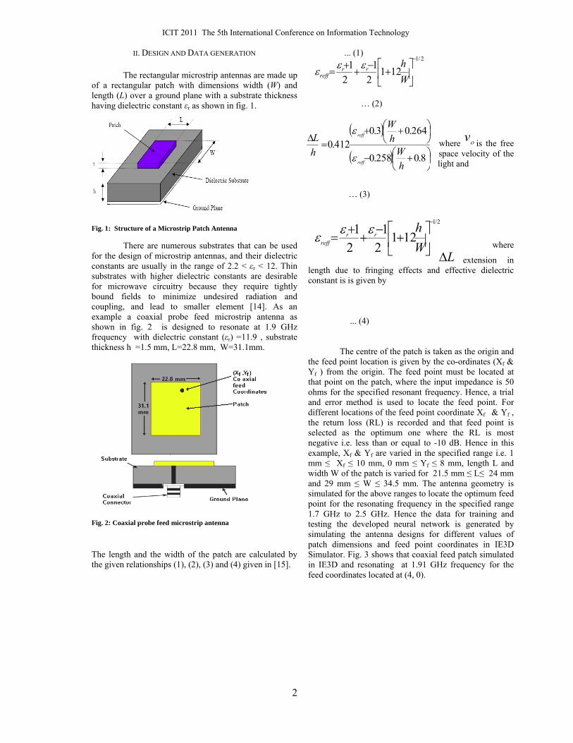
II. DESIGN AND DATA GENERATION

The rectangular microstrip antennas are made up of a rectangular patch with dimensions width (W) and length (L) over a ground plane with a substrate thickness having dielectric constant εr as shown in fig. 1.

Fig. 1: Structure of a Microstrip Patch Antenna

There are numerous substrates that can be used for the design of microstrip antennas, and their dielectric constants are usually in the range of 2.2 < εr < 12. Thin substrates with higher dielectric constants are desirable for microwave circuitry because they require tightly bound fields to minimize undesired radiation and coupling, and lead to smaller element [14]. As an example a coaxial probe feed microstrip antenna as shown in fig. 2 is designed to resonate at 1.9 GHz frequency with dielectric constant (εr) =11.9 , substrate thickness h =1.5 mm, L=22.8 mm, W=31.1mm.

Fig. 2: Coaxial probe feed microstrip antenna The length and the width of the patch are calculated by the given relationships (1), (2), (3) and (4) given in [15].

... (1)

… (2)

where οv is the free space velocity of the light and

… (3)

where

L∆ extension in length due to fringing effects and effective dielectric constant is is given by

... (4) The centre of the patch is taken as the origin and

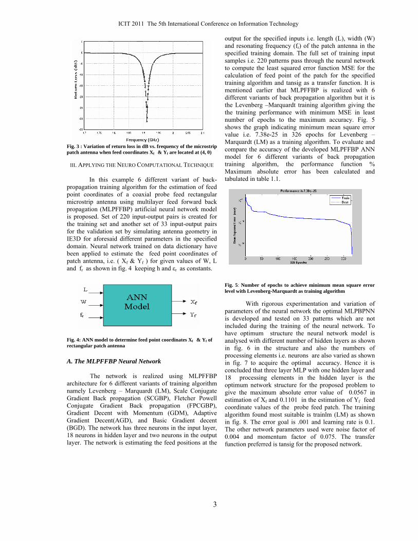
the feed point location is given by the co-ordinates (Xf & Yf ) from the origin. The feed point must be located at that point on the patch, where the input impedance is 50 ohms for the specified resonant frequency. Hence, a trial and error method is used to locate the feed point. For different locations of the feed point coordinate Xf & Yf , the return loss (RL) is recorded and that feed point is selected as the optimum one where the RL is most negative i.e. less than or equal to -10 dB. Hence in this example, Xf & Yf are varied in the specified range i.e. 1 mm ≤ Xf ≤ 10 mm, 0 mm ≤ Yf ≤ 8 mm, length L and width W of the patch is varied for 21.5 mm ≤ L≤ 24 mm and 29 mm ≤ W ≤ 34.5 mm. The antenna geometry is simulated for the above ranges to locate the optimum feed point for the resonating frequency in the specified range 1.7 GHz to 2.5 GHz. Hence the data for training and testing the developed neural network is generated by simulating the antenna designs for different values of patch dimensions and feed point coordinates in IE3D Simulator. Fig. 3 shows that coaxial feed patch simulated in IE3D and resonating at 1.91 GHz frequency for the feed coordinates located at (4, 0).

ICIT 2011 The 5th International Conference on Information Technology

3

Fig. 3 : Variation of return loss in dB vs. frequency of the microstrip patch antenna when feed coordinates Xf & Yf are located at (4, 0)

III. APPLYING THE NEURO COMPUTATIONAL TECHNIQUE

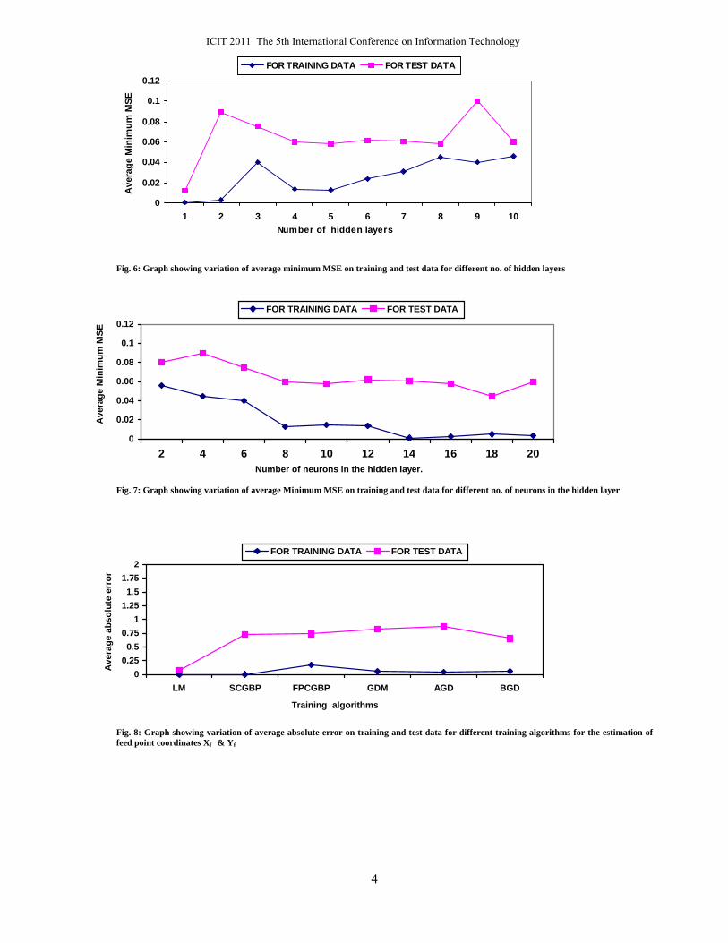
In this example 6 different variant of back-propagation training algorithm for the estimation of feed point coordinates of a coaxial probe feed rectangular microstrip antenna using multilayer feed forward back propagation (MLPFFBP) artificial neural network model is proposed. Set of 220 input-output pairs is created for the training set and another set of 33 input-output pairs for the validation set by simulating antenna geometry in IE3D for aforesaid different parameters in the specified domain. Neural network trained on data dictionary have been applied to estimate the feed point coordinates of patch antenna, i.e. ( Xf & Yf ) for given values of W, L and fr as shown in fig. 4 keeping h and εr as constants.

Fig. 4: ANN model to determine feed point coordinates Xf & Yf of rectangular patch antenna A. The MLPFFBP Neural Network

The network is realized using MLPFFBP

architecture for 6 different variants of training algorithm namely Levenberg – Marquardt (LM), Scale Conjugate Gradient Back propagation (SCGBP), Fletcher Powell Conjugate Gradient Back propagation (FPCGBP), Gradient Decent with Momentum (GDM), Adaptive Gradient Decent(AGD), and Basic Gradient decent (BGD). The network has three neurons in the input layer, 18 neurons in hidden layer and two neurons in the output layer. The network is estimating the feed positions at the

output for the specified inputs i.e. length (L), width (W) and resonating frequency (fr) of the patch antenna in the specified training domain. The full set of training input samples i.e. 220 patterns pass through the neural network to compute the least squared error function MSE for the calculation of feed point of the patch for the specified training algorithm and tansig as a transfer function. It is mentioned earlier that MLPFFBP is realized with 6 different variants of back propagation algorithm but it is the Levenberg –Marquardt training algorithm giving the the training performance with minimum MSE in least number of epochs to the maximum accuracy. Fig. 5 shows the graph indicating minimum mean square error value i.e. 7.38e-25 in 326 epochs for Levenberg – Marquardt (LM) as a training algorithm. To evaluate and compare the accuracy of the developed MLPFFBP ANN model for 6 different variants of back propagation training algorithm, the performance function % Maximum absolute error has been calculated and tabulated in table 1.1.

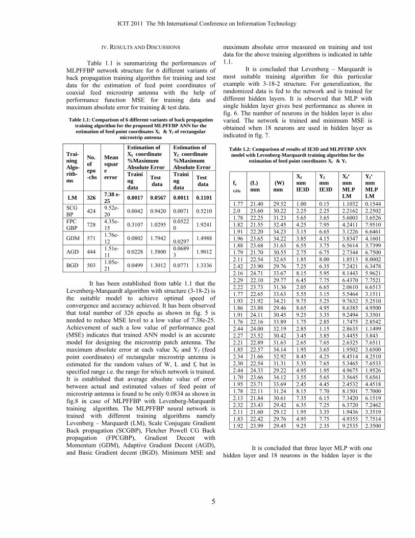
Fig. 5: Number of epochs to achieve minimum mean square error level with Levenberg-Marquardt as training algorithm With rigorous experimentation and variation of parameters of the neural network the optimal MLPBPNN is developed and tested on 33 patterns which are not included during the training of the neural network. To have optimum structure the neural network model is analysed with different number of hidden layers as shown in fig. 6 in the structure and also the numbers of processing elements i.e. neurons are also varied as shown in fig. 7 to acquire the optimal accuracy. Hence it is concluded that three layer MLP with one hidden layer and 18 processing elements in the hidden layer is the optimum network structure for the proposed problem to give the maximum absolute error value of 0.0567 in estimation of Xf and 0.1101 in the estimation of Yf feed coordinate values of the probe feed patch. The training algorithm found most suitable is trainlm (LM) as shown in fig. 8. The error goal is .001 and learning rate is 0.1. The other network parameters used were noise factor of 0.004 and momentum factor of 0.075. The transfer function preferred is tansig for the proposed network.

ICIT 2011 The 5th International Conference on Information Technology

4

Fig. 6: Graph showing variation of average minimum MSE on training and test data for different no. of hidden layers

Fig. 7: Graph showing variation of average Minimum MSE on training and test data for different no. of neurons in the hidden layer

Fig. 8: Graph showing variation of average absolute error on training and test data for different training algorithms for the estimation of feed point coordinates Xf & Yf

0

0.02

0.04

0.06

0.08

0.1

0.12

1 2 3 4 5 6 7 8 9 10 Number of hidden layers

Ave

rage

Min

imum

MSE

FOR TRAINING DATA FOR TEST DATA

0

0.02

0.04

0.06

0.08

0.1

0.12

2 4 6 8 10 12 14 16 18 20Number of neurons in the hidden layer.

Ave

rage

Min

imum

MSE

FOR TRAINING DATA FOR TEST DATA

00.250.5

0.751

1.251.5

1.752

LM SCGBP FPCGBP GDM AGD BGD

Training algorithms

Ave

rage

abs

olut

e er

ror

FOR TRAINING DATA FOR TEST DATA

ICIT 2011 The 5th International Conference on Information Technology

5

IV. RESULTS AND DISCUSSIONS

Table 1.1 is summarizing the performances of MLPFFBP network structure for 6 different variants of back propagation training algorithm for training and test data for the estimation of feed point coordinates of coaxial feed microstrip antenna with the help of performance function MSE for training data and maximum absolute error for training & test data.

Table 1.1: Comparison of 6 different variants of back propagation

training algorithm for the proposed MLPFFBP ANN for the estimation of feed point coordinates Xf & Yf of rectangular

microstrip antenna

It has been established from table 1.1 that the

Levenberg-Marquardt algorithm with structure (3-18-2) is the suitable model to achieve optimal speed of convergence and accuracy achieved. It has been observed that total number of 326 epochs as shown in fig. 5 is needed to reduce MSE level to a low value of 7.38e-25. Achievement of such a low value of performance goal (MSE) indicates that trained ANN model is an accurate model for designing the microstrip patch antenna. The maximum absolute error at each value Xf and Yf (feed point coordinates) of rectangular microstrip antenna is estimated for the random values of W, L and fr but in specified range i.e. the range for which network is trained. It is established that average absolute value of error between actual and estimated values of feed point of microstrip antenna is found to be only 0.0834 as shown in fig.8 in case of MLPFFBP with Levenberg-Marquardt training algorithm. The MLPFFBP neural network is trained with different training algorithms namely Levenberg – Marquardt (LM), Scale Conjugate Gradient Back propagation (SCGBP), Fletcher Powell CG Back propagation (FPCGBP), Gradient Decent with Momentum (GDM), Adaptive Gradient Decent (AGD), and Basic Gradient decent (BGD). Minimum MSE and

maximum absolute error measured on training and test data for the above training algorithms is indicated in table 1.1. It is concluded that Levenberg – Marquardt is most suitable training algorithm for this particular example with 3-18-2 structure. For generalization, the randomized data is fed to the network and is trained for different hidden layers. It is observed that MLP with single hidden layer gives best performance as shown in fig. 6. The number of neurons in the hidden layer is also varied. The network is trained and minimum MSE is obtained when 18 neurons are used in hidden layer as indicated in fig. 7.

Table 1.2: Comparison of results of IE3D and MLPFFBP ANN model with Levenberg-Marquardt training algorithm for the

estimation of feed point coordinates Xf & Yf

It is concluded that three layer MLP with one hidden layer and 18 neurons in the hidden layer is the

Estimation of Xf coordinate %Maximum Absolute Error

Estimation of Yf coordinate %Maximum Absolute Error

Trai-ning Algo-rith-ms

No.of epo-chs

Mean square error Traini

ng data

Test data

Training data

Test data

LM 326 7.38 e-25 0.0017 0.0567 0.0011 0.1101

SCGBP 424 9.52e-

20 0.0042 0.9420 0.0071 0.5210

FPCGBP 728 4.35e-

15 0.3107 1.0295 0.05220 1.9241

GDM 571 1.76e-12 0.0802 1.7942

0.0297 1.4988

AGD 444 1.51e-11 0.0228 1.5800 0.0689

3 1.9012

BGD 503 1.05e-21 0.0499 1.3012 0.0771 1.3336

fr

GHz (L) mm

(W) mm

Xf mm IE3D

Yf mm IE3D

Xf‘ mm MLP LM

Yf‘ mm MLP LM

1.77 21.40 29.52 1.00 0.15 1.1032 0.1544 2.0 23.60 30.22 2.25 2.25 2.2162 2.2502 1.78 22.25 31.23 5.65 3.65 5.6003 3.6526 1.82 21.55 32.45 4.25 7.95 4.2411 7.9510 1.91 22.20 34.23 3.15 6.65 3.1226 6.6461 1.96 23.65 34.22 3.85 4.15 3.8347 4.1601 1.88 23.68 31.63 6.55 3.75 6.5614 3.7399 1.79 21.70 30.55 2.75 6.75 2.7344 6.7500 2.11 22.54 32.65 1.85 8.00 1.8513 8.0002 2.42 23.90 29.76 7.25 6.35 7.2421 6.3478 2.16 24.71 33.67 8.15 5.95 8.1443 5.9621 2.29 22.10 29.77 6.45 7.75 6.4370 7.7521 2.22 23.73 31.36 2.05 6.65 2.0610 6.6513 1.77 22.65 33.63 5.55 3.15 5.5464 3.1511 1.93 21.92 34.21 9.75 5.25 9.7632 5.2510 1.86 23.88 29.46 8.65 4.95 8.6385 4.9500 1.91 24.11 30.45 9.25 3.35 9.2494 3.3501 1.76 22.16 33.89 1.75 2.85 1.7475 2.8542 2.44 24.00 32.19 2.85 1.15 2.8635 1.1499 2.27 23.52 30.42 3.45 3.85 3.4455 3.843 2.21 22.89 31.63 2.65 7.65 2.6325 7.6511 1.85 22.57 34.14 1.95 3.65 1.9502 3.6500 2.34 21.66 32.92 8.45 4.25 8.4514 4.2510 2.30 22.54 31.31 5.35 7.65 5.3465 7.6533 2.44 24.33 29.22 4.95 1.95 4.9675 1.9526 1.70 23.66 34.12 3.55 5.65 3.5645 5.6561 1.95 23.71 33.69 2.45 4.45 2.4532 4.4518 1.78 22.11 31.24 8.15 7.70 8.1501 7.7000 2.13 21.84 30.61 7.35 6.15 7.3420 6.1519 2.32 23.43 29.42 6.35 7.25 6.3720 7.2462 2.11 21.60 29.12 1.95 3.35 1.9436 3.3519 1.83 22.42 29.76 4.95 7.75 4.9355 7.7514 1.92 23.99 29.45 9.25 2.35 9.2535 2.3500

ICIT 2011 The 5th International Conference on Information Technology

6

optimum network structure for the proposed problem to give the maximum absolute error value of 0.0567 in estimation of Xf and 0.1101 in the estimation of Yf which is minimum amongst the mentioned 6 variants of back propagation training algorithm. Table 1.2 shows the comparison of results obtained from MLPFFBP ANN model with Levenberg-Marquardt (LM) training algorithm for the estimation of feed point coordinates for the aforesaid network structure.

V. CONCLUDING REMARKS

The developed MLPFFBP ANN model is

estimating the feed point coordinate Xf to the accuracy of 99.94 % and Yf coordinate to the accuracy of 99.88% with Levenberg – Marquardt training algorithm. In the literature no such analysis is reported so far for the determination feed point coordinates of a coaxial feed microstrip antenna. Henceforth the developed MLPFFBP with Levenberg - Marquardt training algorithm and the aforesaid structure is estimating the feed point coordinates quite satisfactory in comparison to simulation findings from IE3D simulator.

REFERENCES

[1] P.M. Watson, K.C. Gupta, “Design and Optimization of CPW Circuits Using EM ANN Models for CPW Components”, IEEE Transactions on Microwave Theory and Techniques, vol. 45, no. 12, pp. 2515 – 2523, 1997.

[2] A. H. Zaabab, Q.J. Zhang, M. Nakhla,” Analysis and Optimization of Microwave Circuits & Devices Using Neural Network Models”, IEEE MTT-S Digest 1994, pp 393- 396, 1994.

[3] Q. J. Zhang, K. C. Gupta, “Neural Networks for RF and Microwave Design”, Artech House Publishers, 2000.

[4] Simon Haykins, “Neural networks”, second edition, pHI, 2000. [5] J. Lakshmi Narayana, K. Sri Rama Krishna and L. Pratap

Reddy, “Design of microstrip antennas using artificial neural networks”, International Conference on ComputationalIntelligence and Multimedia Applications 2007, pp.332-334, 2007.

[6] Nurhan Turker, Filiz Gunes and Tulay Yildirim ,”Artificial neural design of microstrip antennas”, Turk J. Elec. Engin., vol. 14, no.3, pp.445-453, 2006.

[7] F. Peik, G. Coutts, R. R. Mansour, Application of neural networks in microwave circuit modeling ,Electrical and computer Engineering,1998,IEEE Canadian Conference ,vol-2,24-28 , , pp. 928-931, May 1998.

[8] S. Devi, D. C. Panda and S. S. Pattnaik, “A novel method of using artificial neural networks to calculate input impedance of circular microstrip antenna”, Antennas and Propagation Society International Symposium, vol.3, pp. 462– 465, 2002.

[9] R. K. Mishra and A. Patnaik, “Neural network- based CAD model for the design of square-patch antennas, IEEE Transactions on Antennas and Propagation, vol. 46, no.12, pp.1890–1891, 1998.

[10] A. Patnaik, R. K. Mishra, G. K. Patra and S. K. Dash, “An artificial neural network model for effective dielectric constant of microstrip line”, IEEE Trans. on Antennas Propagation., vol.45, no.11, pp.1697, 1997.

[11] D. Karaboga, K. Guney, S. Sagiroglu and M. Erler, “Neural computation of resonant frequency of electrically thin and thick rectangular microstrip antenna”, Microwaves, Antennas and Propagation, IEEE Proc. vol.146, no.2, pp.155- 156, 1999.

[12] S. Sagiroglu, K. G uney and M. Erler, “Resonant frequency calculation for circular microstrip antennas using artificial neural networks”, International Journal of RF and Microwave Computer Aided Engineering, vol. 8, no.3, pp. 270- 277, 1998.

[13] IE3D Software Release-8, Developed by M/S Zeland Software Inc.

[14] D. M. Pozar, “Microstrip Antennas, Proc. IEEE”, vol. 80, no.1, pp.79- 81, 1992.

[15] C. A. Balanis, “Antenna theory”, John Wiley & Sons, Inc.,1997

ICIT 2011 The 5th International Conference on Information Technology