An Integration of Solow’s Growth and Dixit-Stiglitz’s ...

University of Piraeus

SPOUDAI Journal of Economics and Business

Σπουδαί http://spoudai.unipi.gr

An Integration of Solow’s Growth and Dixit-Stiglitz’s Monopolistic Competition Models

Prof. Wei-Bin Zhang

Ritsumeikan Asia Pacific University, Japan E-mail: [email protected]

Abstract: This study proposes an economic growth model with perfectly competitive and monopolistic competitive market structures. Our model is based on two core models in two mainstreams of economic theories. One is the Solow model in neoclassical growth theory. The other one is the Dixit-Stiglitz model of monopolistic competition. The unique contribution of this research is to integrate the two models in a comprehensive framework. It endogenously determines profit which is equally distributed among the homogeneous population. We examine the role of perfect competition and monopolistic competition in economic growth. We build and then simulate the model. We find a unique equilibrium point and confirm stability. We plot the motion of the economy and conduct comparative dynamic analyses to get some insights into the complexity of economic growth.

Keywords: Solow model; monopolistic competition; Dixit-Stiglitz model; wealth accumulation; profit. JEL Classification: D110; O41; L130.

Acknowledgements: The author is grateful to the important comments of Prof. E. Sambracos.

1. IntroductionEconomic development is a complicated issue. Different economies have different markets and experience different paths of development in modern times. There are different economic theories which are proposed for analyzing economic phenomena of different economic systems. The purpose of this study is to integrate two core models of the two mainstreams in the literature of economic theory. The two mainstreams are respectively neoclassical growth theory and economic equilibrium with monopolistic completion. The two core models are respectively Solow’s one-sector growth model (Solow, 1956) and Dixit-Stiglitz’s equilibrium model with monopolistic competition (Dixit and Stiglitz, 1977). A main deviation of this paper from the mainstreams of economics is the application of Zhang’s concept of disposable income and utility in modelling behavior of households (Zhang, 1993, 2005).

Capital is an important determinant of modern economic growth. Neoclassical growth theory is the main economic theory which explicitly deals with endogenous wealth accumulation with microeconomic foundation. The theory mainly deals with economic theory with capital as the main machine of economic growth. Its core model – Solow’s one sector growth model - outlines how the economic growth rate is determined with exogenous saving and exogenous population growth under the conditions that all markets are perfectly competitive. The final goods sector in this study is based on the Solow model. The Solow model is built for a perfectly competitive market with wealth/capital accumulation. Wealth accumulation is the main machine of

3

SPOUDAI Journal of Economics and Business, Vol.68 (2018), Issue 4 , pp. 3-19

economic growth with exogenous population and technological changes. The Solow model is the core model of neoclassical growth theory in the sense that most of the models in the literature are extensions and generalizations of the Solow growth model (e.g., Solow, 1956; Burmeister and Dobell, 1970; Azariadis, 1993; Barro and Sala-i-Martin, 1995; Ben-David and Loewy, 2003, and Zhang, 2005, 2008). There are some extensions of the Solow model by including endogenous population or/and environment, this study deviates from the previous studies by introducing monopolistic competition to neoclassical growth theory by applying the modelling strategy by Dixit and Stiglitz (1977) and the literature of economic equilibrium with monopolistic competition (Lancaster, 1980; Benassy, 1996; Picard and Toulemonde, 2009; Wang, 2012; Bertoletti and Etro, 2015; Nocco, et. al., 2017; and Parenti, et.al., 2017). It should be noted that a main problem of the Solow model is the lacking of microeconomic foundation for analyzing household decisions on saving and time distribution. This studies overcomes this problem by accepting an alternative approach to household behavior.

Some markets in real economies are not perfectly competitive as assumed in standard neoclassical growth theory and standard general equilibrium economic theory. There are many economic behavior, which cannot be characterized by perfect competition due to market structures and imperfect information. This study is focused on monopolistic completion, which is characterized by many producers who produce differentiated products. Products are differentiated from each other and are not perfect substitutes. Each firm takes the prices charged by other firms as given and maximizes its profit. Each firm has some degree of market power, which is measured by controlling power over the terms and conditions of demand and supply equilibrium. Theory of monopolistic competition is initiated by Chamberlin (1933). The concept of monopolistic competition as a market structure has increasingly played important role in modelling modern economic structures, economic growth and development, economic geography, as well as innovation and technological diffusion (e.g., Neary, 2001; Brakman and Heijdra, 2004; Behrens and Murata, 2007; Behrens and Murata, 2009; Demidova, 2017). An early model in the literature of monopolistic completion is developed by Dixit and Stiglitz (1977). The model has led to development of many models in subfields of economics (e.g., Krugman, 1979; Ethier, 1982; Romer, 1990; Wang, 2012). It should be noted that rather than strictly following the Dixit-Stiglitz model in modelling monopolistic competition, we follow Grossman and Helpman (1990) in that intermediate goods are used as inputs of the final goods sector rather than consumer goods in the Dixit-Stiglitz model. We differ from the Grossman-Helpman model in that the profits of intermediate inputs sectors are distributed among the homogeneous population rather than are used for innovation. In particular, we apply Zhang’s concept of disposable income and utility function to model behavior of the household. The rest of the paper is organized as follows. Section 2 builds the growth model of perfect competition and monopolistic competition on the basis of the Solow model and the Dixit-Stiglitz model. Section 3 studies analytical properties of the model and simulates the model. Section 4 carries out comparative dynamic analysis in a few parameters. Section 5 concludes the study.

2. The neoclassical growth model with intermediate inputs The model is basically a combination of the Solow one-sector neoclassical growth model, the Dixit-Stiglitz model with product variety and Zhang’s concept of disposable income and utility function. On the basis of the modeling framework by Dixit and Stiglitz (1997, see also Grossman and Helpman, 1990), we consider that the supply side consists of two kinds of activities: the production of a final good and the production of a variety of differentiated middle products (i.e., intermediate inputs). The final product is like the commodity in the Solow model, which can be invested as capital good and consumed as consumer good. Capital is used as inputs in the production of final product. We deviate from the Grossman and Helpman approach in

4

Wei-Bin Zhang, SPOUDAI Journal, Vol.68 (2018), Issue 4 , pp. 3-19

which endogenous capital is neglected and follow Solow model in that capital accumulation is the engine of economic growth. Labor is distributed between production of final goods and intermediate inputs.

The production of final product

We use ( ),tFi ( )tK and ( )tNi to represent respectively output of the final goods sector, capital

input and labor input. We use ( )tX i to stand for the (aggregate) input of intermediate inputs ofthe sector as follows:

( ) ( ) ,10,1

<<= ∑=

θε

θε

n

i txtX (1)

in which ( )txε stands for the input of middle product ,ε n is the number of varieties of middle products available, and θ is a parameter. Following Grossman and Helpman (1990), we specify a production function of final goods as follows:

( ) ( ) ( ) ( ) ,11,1,,0, <−−

=<+<=θ

βαγβαβαγβα iiiiiiiiiii tXtNtKAtF iii (2)

where ,iA iα and iβ are parameters. The production function exhibits constant returns to scale for given n , but exhibits an increase in .n This function shows that an increasing degree of specialization enhances technical efficiency as a rise in .n Developing new middle products implies increasing the degree of specialization. This implies that there exist scale economies at the industry level that are exogenous to the individual firms in the final goods sector.

We assume that the final good serves as a medium of exchange and is taken as numeraire. We assume that capital depreciates at a constant exponential rate δ k . We denote ( ),tw ( ),tr and

( ),tpε the wage rate, the rate of interest, and the price of middle good .ε The profit of the final goods sector is

( ) ( ) ( )( ) ( ) ( ) ( ) ( ) ( ).1

∑=

−−+−=n

ikii txtptNtwtKtrtFtε

εεδπ

The marginal conditions are

( ) ( )( ) ( ) ( )

( ) ( ) ( ) ( )( ) .,,

1

tXtFtxtp

tNtFtw

tKtFtr

i

ii

i

iiiik

−

===+θε

εθγβαδ (3)

The share of factor iX is .ii Fγ From (2) and the marginal conditions for capital and labor in (3) we solve

( ) ( ) ( ) ( ) ( )( ) ( )

( )

,,1/1 −

=Λ=

i

ii tXtKAtwtNtXttK

iiiii

β

γαβ(4)

where

5


( ) ( )( ) ( ) ( ) .,,,

/11

kii

ii

trtrtwA

Atrtwr

iii

δβα δ

γββ

δ +≡

≡Λ

−

The Function ( )tΛ is independent of variety. From (3), we also have

( ) ( ) ( ) ( )( ) .1

tXtKtxtrtp

ii

ii

αθγ θ

εδε

−

= (5)

Insert (4) in (5)

( ) ( ) ( ),~ tpttx θεε−Λ= (6)

where

( ) ( ) ( ) .1

1,~θ

θα

θγθ

δ

−≡

Λ≡Λ

i

ii ttrt

It should be noted that ( )tΛ~ is independent of variety. The share of variety ε in terms of the total value of intermediate inputs is

( ) ( ) ( )( ) ( )

.1∑ =

≡ n

m mm tptxtptxt εε

εφ (7)

Insert (6) in (7)

( ) ( )( )

.1

1

1

∑ =−

−

= n

m m tptptθ

θε

εφ (8)

The middle goods sector At each point of time production of middle goods is characterized of oligopolistic price competition. The profit comprises the product of profits per unit of product and the share of the market. The producer of variety ε chooses ( )tpε to maximizes the following profit:

( ) ( ) ( )[ ] ( ) ( )( ) ,tp

tFttwatpt iiN

ε

εεε

γφπ −=

where Na is the unit labor requirement for production of intermediates. Insert (8) in the above equation

6


( ) ( ) ( )[ ] ( ) ( )( )

,1

1∑ =−

−

−= n

m m

iiN

tptptFtwatpt

θ

θε

εεγπ (9)

From (3) and (1), we have

( ) ( )( ) ( ).

11 ∑

=−=

n

ii tx

txtptF

ε

θεθ

ε

ε

θγ(10)

Insert (6) in (10)

( )( )

( ).~

11 θγθ

in

m m

i ttp

tF Λ=

∑ =− (11)

From (9) and (11), we have the profit function as follows:

( ) ( ) ( )[ ] ( ) ( ).~

θγγπ

θε

εεi

iN

tpttwatpt−Λ

−=

The first-order condition (i.e., 0/ =∂∂ εεπ p ) of the above implies the following fixed-markup pricing rule:

( ) ( ).twatp N=εθ (12)

This equation also implies that the price is independent of variety. Varieties bear the same price. With (9) and (12), the profit per firm is:

( ) ( ) ( ) ,1n

tFt iiγθπ −= (13)

which is independent of .ε From (5), we also conclude that ( )txε is independent of ,ε denoted by ( ).tx From (1) we have

( ) ( ).txntX ii

θ= (14)

The total profit is

( ) ( ).tnt ππ = (15)

Consumer behaviors and wealth dynamics In this study, we use an alternative approach to modeling behavior of households proposed by Zhang (1993, 2005, 2014). Let ( )tk stand for per capita wealth. We have ( ) ( ) ,/ NtKtk = where

( )tK is the total capital. We assume that the profit is equally shared among households. Itshould be noted that in neo growth theory profit is often invested for innovation. This study

7


assumes profit to be shared equally between the homogenous households. A more general approach should specify different possible distributions of profits among firms, households and governments (for instance, in form of taxation). We take a simplified approach at this initial stage of modelling. We use ( )tT and ( )tT to stand for, respectively, work time andleisure time. The household’s time constraint is

( ) ( ) .0TtTtT =+ (16)

Let h stand for human capital. The current income of the representative household is

( ) ( ) ( ) ( ) ( ) ( ).N

ttTtwhtktrty π++= (17)

The household disposable income ( )ty is the sum of the current disposable income and thevalue of wealth as follows:

( ) ( ) ( ) ( ) ( ) ( ),ˆ tTtwhtytktyty −=+= (18)

where ( ) ( )tTtwh is the opportunity cost of leisure and ( )ty is the disposable income when thehousehold spends all the available time on work:

( ) ( )( ) ( ) ( ) ( ).1 0 NtTtwhtktrty π

+++=

The representative household distributes the total available budget between savings ( )ts and consuming goods ( ).tc The budget constraint is

( ) ( ) ( ).ˆ tytstc =+ (19)


( ) ( ) ( ) ( ) ( ).tytstctTtwh =++ (20)

In our model the household decides consumption level, saving, and leisure time. We assume that utility level ( )tU is dependent on ( ),tT ( )tc and ( )ts as follows

8


( ) ( ) ( ) ( ) ,0,,, 000000 >= λξσλξσ tstctTtU

where 0σ is the propensity to use leisure time, 0ξ is the propensity to consume goods, and 0λthe propensity to save. Maximizing the utility subject to (20) yields

( ) ( ) ( ) ( ) ( ) ( ) ( ),,, tytstytctytTtw λξσ === (21)

where

.1,,,000

000

λξσρλρλξρξσρσ

++≡≡≡≡

h

According to the definition of ( )ts , the change in the household’s wealth is given by

( ) ( ) ( ) ( ) ( ).tktytktstk −=−= λ (22)

This equation simply states that the change in wealth is equal to savings minus dissavings.

Demand and supply of final goods As change in capital stock equal to the output of the final goods sector is minus the depreciation of capital stock and total consumption, we have

( ) ( ) ( ) ( ),tKtCtFtK ki δ−−= (23)

where ( ) ( ) .NtctC =

Labor being fully utilized The labor market clearing conditions equate labor supply and labor demand. We have

( ) ( ) ( ) .NtThntxatN Ni =+ (24)

We built the model. The model is based on the Solow model, the modeling framework by Dixit-Stiglitz model, and the Grossman-Helpman model with Zhang’s concept of disposable income and utility function. We now study properties of the model.

9


3. The Dynamic Properties of the ModelThe previous section a neoclassical growth model with monopolistic competition. We now provide a computational program to plot the movement of the economic system.

Lemma The dynamics of the economic system is given by following differential equation:

( ) ( )( ) ( )( ),1

txfxd

txvdtx−

= (25)

where functions ( )( )txv and ( )( )txf are defined in the Appendix. All the other variables areexplicitly given as functions of ( )tx as follows: ( )tk with (A13) → ( ) ( )NtktK = → ( )tFi by (A10) → ( )tw by (A11) → ( )ty by (A6) → ( )tr by (A14) → ( )tT by (A5) → ( ),tT ( )tcand ( )ts by (21) → ( )tπ by (13) → ( )tπ by (13) → ( )tX i by (14) → ( )tpε by (A2) →

( )tφ by (8) → ( )tNi by (A4).

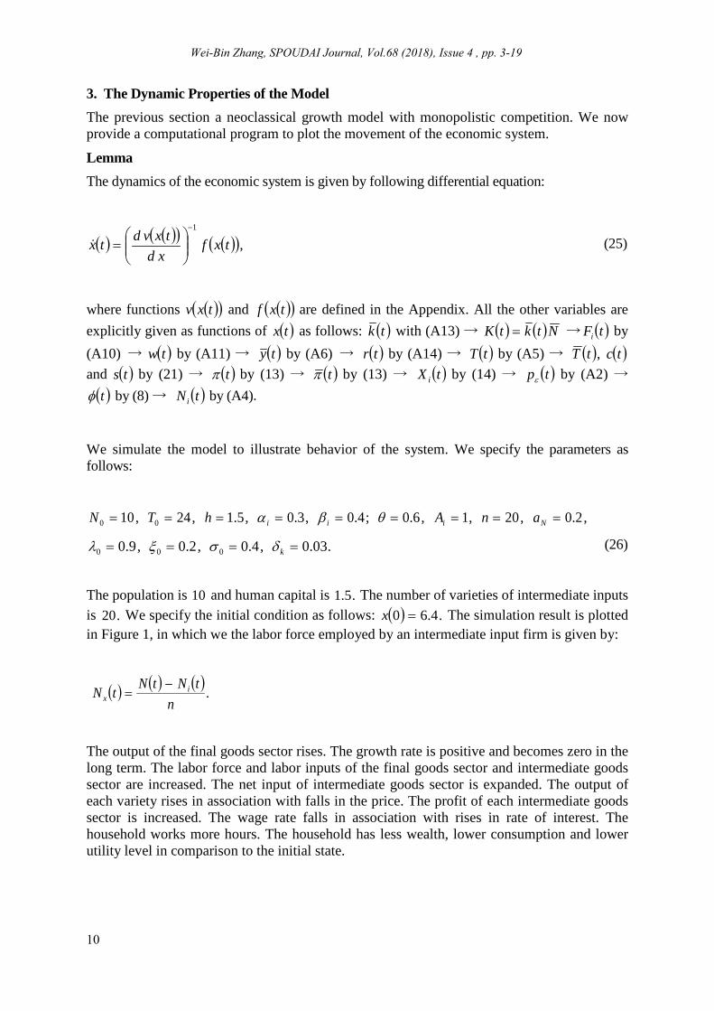
We simulate the model to illustrate behavior of the system. We specify the parameters as follows:

,2.0,20,1,6.0;4.0,3.0,5.1,24,10 00 ========= Niii anAhTN θβα

.03.0,4.0,2.0,9.0 000 ==== kδσξλ (26)

The population is 10 and human capital is .5.1 The number of varieties of intermediate inputs is .20 We specify the initial condition as follows: ( ) .4.60 =x The simulation result is plotted in Figure 1, in which we the labor force employed by an intermediate input firm is given by:

( ) ( ) ( ).

ntNtNtN i

x−

=

The output of the final goods sector rises. The growth rate is positive and becomes zero in the long term. The labor force and labor inputs of the final goods sector and intermediate goods sector are increased. The net input of intermediate goods sector is expanded. The output of each variety rises in association with falls in the price. The profit of each intermediate goods sector is increased. The wage rate falls in association with rises in rate of interest. The household works more hours. The household has less wealth, lower consumption and lower utility level in comparison to the initial state.

10


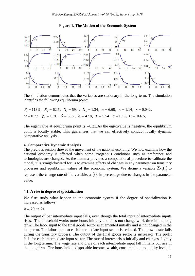
Figure 1. The Motion of the Economic System

The simulation demonstrates that the variables are stationary in the long term. The simulation identifies the following equilibrium point:

,5.166,6.10,54.5,8.47,7.58ˆ,26.0,77.0

,042.0,14.1,68.6,34.1,4.59,5.62,9.113

=======

=======

UcTkypw

rxNNXF xiii

ε

π

The eigenvalue at equilibrium point is .21.0− As the eigenvalue is negative, the equilibrium point is locally stable. This guarantees that we can effectively conduct locally dynamic comparative analysis.

4. Comparative Dynamic AnalysisThe previous section showed the movement of the national economy. We now examine how the national economy is affected when some exogenous conditions such as preference and technologies are changed. As the Lemma provides a computational procedure to calibrate the model, it is straightforward for us to examine effects of changes in any parameter on transitory processes and equilibrium values of the economic system. We define a variable ( )tx j∆ to represent the change rate of the variable, ( ),tx j in percentage due to changes in the parameter value.

4.1. A rise in degree of specialization We fisrt study what happen to the economic system if the degree of specialization is increased as follows:

.2120 ⇒=n

The output of per intermediate input falls, even though the total input of intermediate inputs rises. The household works more hours initially and does not change work time in the long term. The labor input to the final goods sector is augmented initially and is not changed in the long term. The labor input to each intermediate input sector is reduced. The growth rate falls during the transitory process. The output of the final goods sector is increased. The profit falls for each intermediate input sector. The rate of interest rises initially and changes slightly in the long termm. The wage rate and price of each intermediate input fall initially but rise in the long term. The household’s disposable income, wealth, consumption, and utility level all

11


fall initially but rise in the long term. Accordingly, enhanced degree of specialization benefits the national economic growth and household’s welfare in the long term, even though the national final goods output rises but the household is worse off in the short term.

Figure 2. A Rise Degree of Specialization

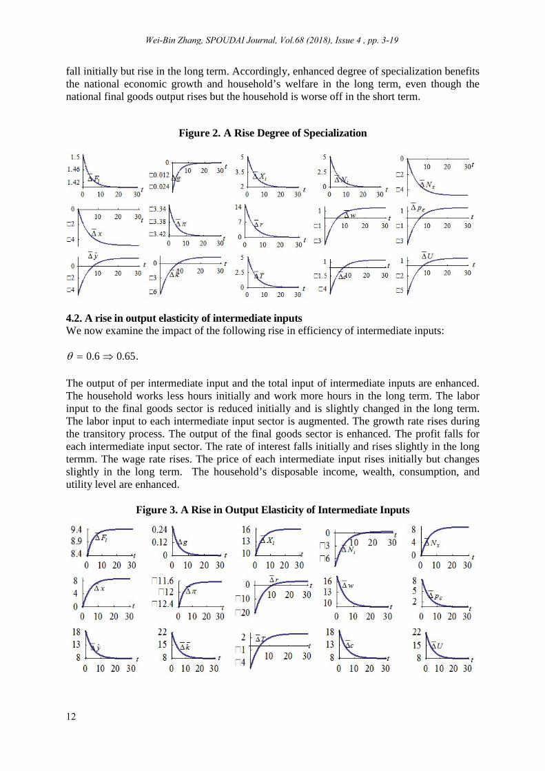
4.2. A rise in output elasticity of intermediate inputs We now examine the impact of the following rise in efficiency of intermediate inputs:

.65.06.0 ⇒=θ

The output of per intermediate input and the total input of intermediate inputs are enhanced. The household works less hours initially and work more hours in the long term. The labor input to the final goods sector is reduced initially and is slightly changed in the long term. The labor input to each intermediate input sector is augmented. The growth rate rises during the transitory process. The output of the final goods sector is enhanced. The profit falls for each intermediate input sector. The rate of interest falls initially and rises slightly in the long termm. The wage rate rises. The price of each intermediate input rises initially but changes slightly in the long term. The household’s disposable income, wealth, consumption, and utility level are enhanced.

Figure 3. A Rise in Output Elasticity of Intermediate Inputs

12


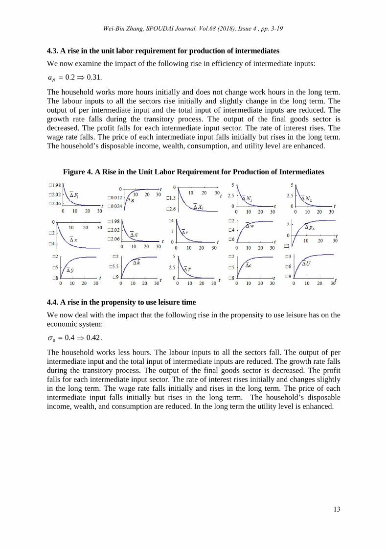
4.3. A rise in the unit labor requirement for production of intermediates We now examine the impact of the following rise in efficiency of intermediate inputs:

.31.02.0 ⇒=Na

The household works more hours initially and does not change work hours in the long term. The labour inputs to all the sectors rise initially and slightly change in the long term. The output of per intermediate input and the total input of intermediate inputs are reduced. The growth rate falls during the transitory process. The output of the final goods sector is decreased. The profit falls for each intermediate input sector. The rate of interest rises. The wage rate falls. The price of each intermediate input falls initially but rises in the long term. The household’s disposable income, wealth, consumption, and utility level are enhanced.

Figure 4. A Rise in the Unit Labor Requirement for Production of Intermediates

4.4. A rise in the propensity to use leisure time We now deal with the impact that the following rise in the propensity to use leisure has on the economic system:

.42.04.00 ⇒=σ

The household works less hours. The labour inputs to all the sectors fall. The output of per intermediate input and the total input of intermediate inputs are reduced. The growth rate falls during the transitory process. The output of the final goods sector is decreased. The profit falls for each intermediate input sector. The rate of interest rises initially and changes slightly in the long term. The wage rate falls initially and rises in the long term. The price of each intermediate input falls initially but rises in the long term. The household’s disposable income, wealth, and consumption are reduced. In the long term the utility level is enhanced.

13


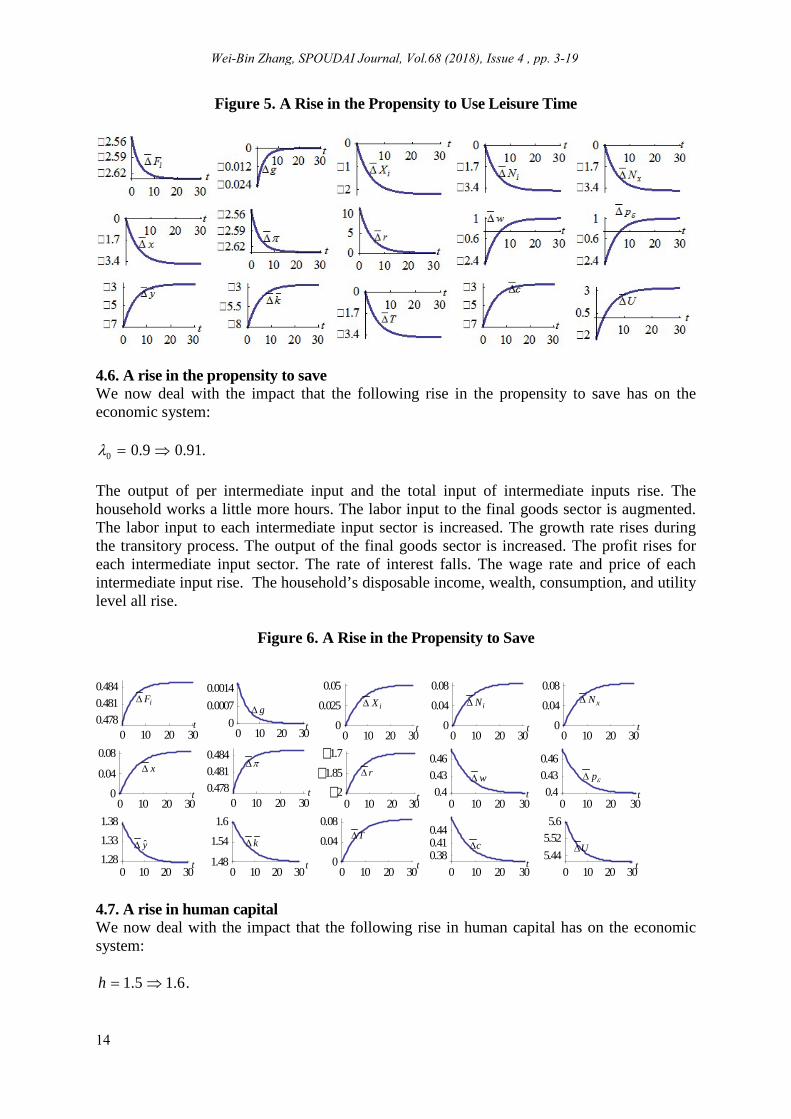
Figure 5. A Rise in the Propensity to Use Leisure Time

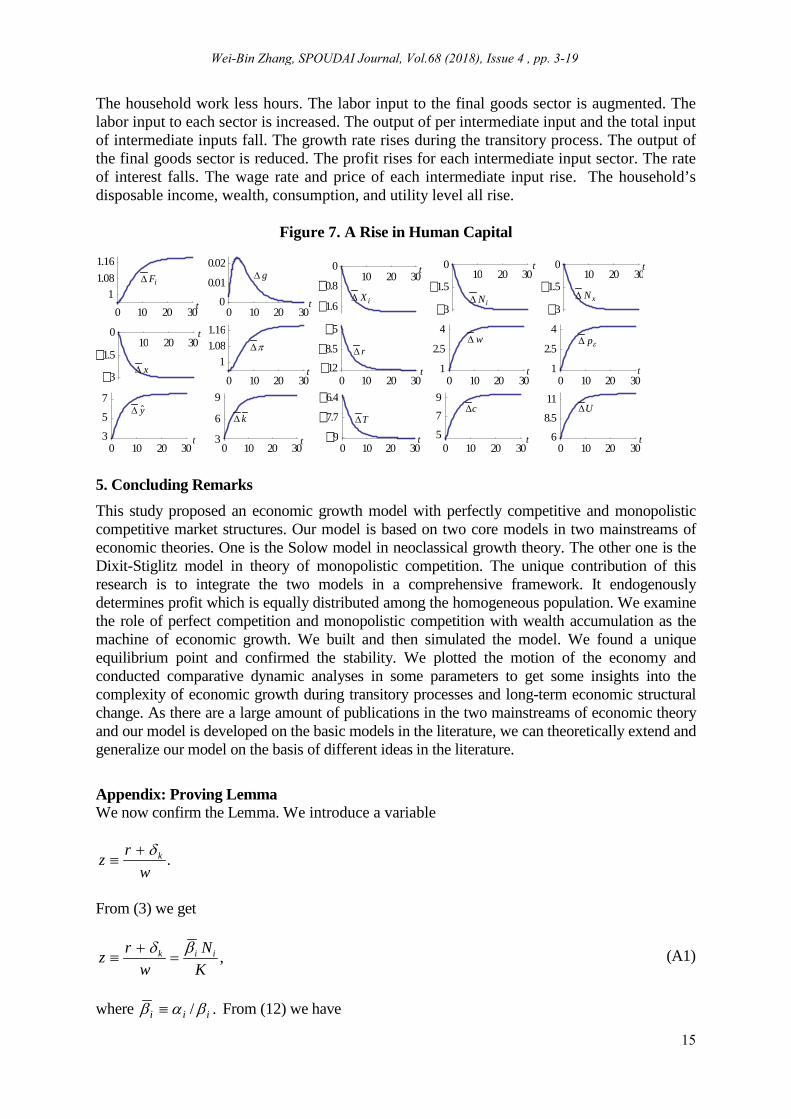
4.6. A rise in the propensity to save We now deal with the impact that the following rise in the propensity to save has on the economic system:

.91.09.00 ⇒=λ

The output of per intermediate input and the total input of intermediate inputs rise. The household works a little more hours. The labor input to the final goods sector is augmented. The labor input to each intermediate input sector is increased. The growth rate rises during the transitory process. The output of the final goods sector is increased. The profit rises for each intermediate input sector. The rate of interest falls. The wage rate and price of each intermediate input rise. The household’s disposable income, wealth, consumption, and utility level all rise.

Figure 6. A Rise in the Propensity to Save

0 10 20 300.4780.4810.484

0 10 20 300

0.00140.0007

0 10 20 300

0.025

0.05

0 10 20 300

0.04

0.08

0 10 20 300

0.04

0.08

0 10 20 300

0.04

0.08

0 10 20 300.4780.4810.484

0 10 20 302

1.85

1.7

0 10 20 300.4

0.430.46

0 10 20 300.4

0.430.46

0 10 20 301.281.331.38

0 10 20 301.48

1.54

1.6

0 10 20 300

0.04

0.08

0 10 20 300.380.410.44

0 10 20 305.445.525.6

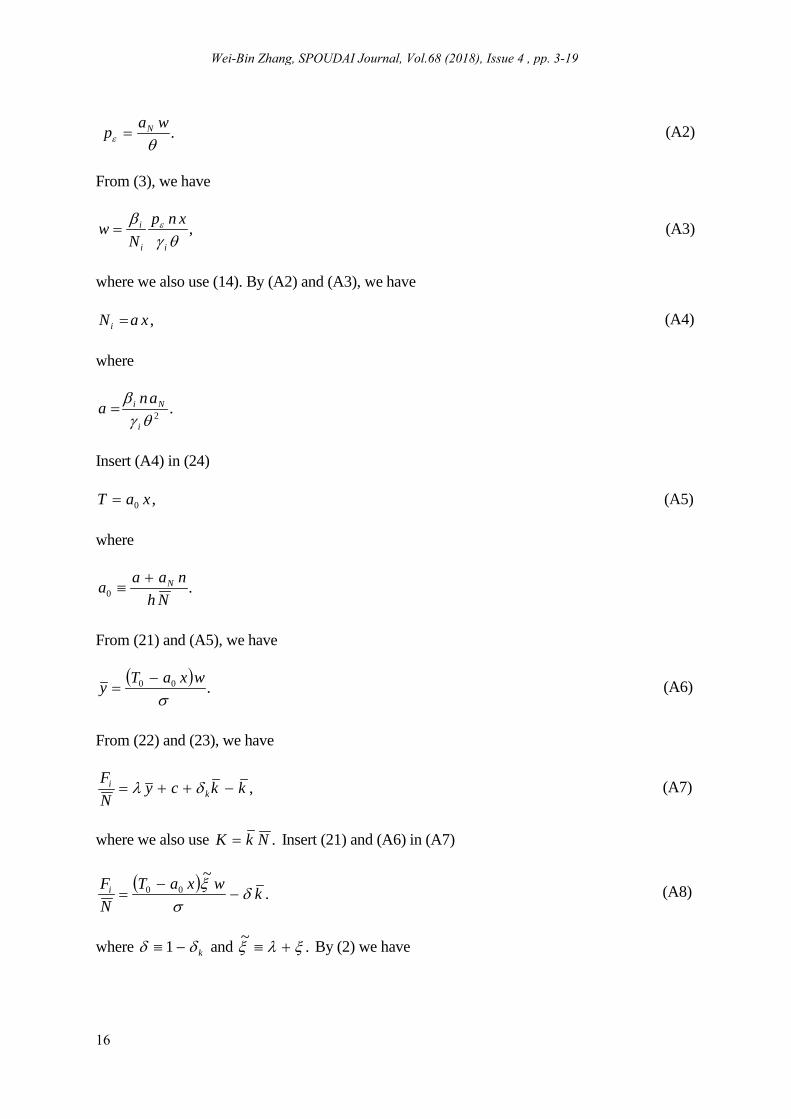
4.7. A rise in human capital We now deal with the impact that the following rise in human capital has on the economic system:

.6.15.1 ⇒=h

xN∆iF∆

r∆

k∆T∆

t

εp∆

g∆

w∆x∆

t t

t

t

t t t

y∆ U∆

π∆

t

ttt

t t

iX∆ iN∆

c∆

t

14


The household work less hours. The labor input to the final goods sector is augmented. The labor input to each sector is increased. The output of per intermediate input and the total input of intermediate inputs fall. The growth rate rises during the transitory process. The output of the final goods sector is reduced. The profit rises for each intermediate input sector. The rate of interest falls. The wage rate and price of each intermediate input rise. The household’s disposable income, wealth, consumption, and utility level all rise.

Figure 7. A Rise in Human Capital

0 10 20 301

1.081.16

0 10 20 300

0.01

0.0210 20 30

1.6

0.8

010 20 30

3

1.5

010 20 30

3

1.5

0

10 20 30

3

1.5

0

0 10 20 30

11.081.16

0 10 20 3012

8.5

5

0 10 20 301

2.5

4

0 10 20 301

2.5

4

0 10 20 303

5

7

0 10 20 303

6

9

0 10 20 309

7.7

6.4

0 10 20 305

79

0 10 20 306

8.5

11

5. Concluding RemarksThis study proposed an economic growth model with perfectly competitive and monopolistic competitive market structures. Our model is based on two core models in two mainstreams of economic theories. One is the Solow model in neoclassical growth theory. The other one is the Dixit-Stiglitz model in theory of monopolistic competition. The unique contribution of this research is to integrate the two models in a comprehensive framework. It endogenously determines profit which is equally distributed among the homogeneous population. We examine the role of perfect competition and monopolistic competition with wealth accumulation as the machine of economic growth. We built and then simulated the model. We found a unique equilibrium point and confirmed the stability. We plotted the motion of the economy and conducted comparative dynamic analyses in some parameters to get some insights into the complexity of economic growth during transitory processes and long-term economic structural change. As there are a large amount of publications in the two mainstreams of economic theory and our model is developed on the basic models in the literature, we can theoretically extend and generalize our model on the basis of different ideas in the literature.

Appendix: Proving Lemma We now confirm the Lemma. We introduce a variable

.w

rz kδ+≡

From (3) we get

,KN

wrz iik βδ

=+

≡ (A1)

where ./ iii βαβ ≡ From (12) we have

xN∆iF∆

r∆

k∆ T∆

t

εp∆

g∆

w∆

x∆

t t

t

t

t t

t

y∆ U∆

π∆

t

ttt

t t

iX∆ iN∆

c∆

t

15


.θε

wap N= (A2)

From (3), we have

,θγ

β ε

ii

i xnpN

w = (A3)

where we also use (14). By (A2) and (A3), we have

,xaNi = (A4)

where

.2θγβ

i

Ni ana =

Insert (A4) in (24)

,0 xaT = (A5)

where

.0 Nhnaaa N+

≡

From (21) and (A5), we have

( ) .00

σwxaTy −

= (A6)


,kkcyNF

ki −++= δλ (A7)

where we also use .NkK = Insert (21) and (A6) in (A7)

( ) .~

00 kwxaTNFi δ

σξ

−−

= (A8)

where kδδ −≡ 1 and .~ ξλξ +≡ By (2) we have

16


.ii

i

i

iiii N

XNKNAF

γα

= (A9)

Insert (A1) and (A4) in (A9)

( ) .,1 ii

axn

zxaAzxF i

ii

γθαβ

=

−

(A10)

From (3), (A10) and (A4), we have

( ) ( ).,,xa

zxFzxw iiβ= (A11)

From (A8) and (A10), we solve

( ) ( ) ( ).,,~00

NzxFzxwxaTk i

δσδξ

−−

=(A12)

Insert (A11) in (A12)

( ) ( ),, zxFxVk i= (A13)

where

( ) ( ) .11~00

δσξβ

−

−≡

NxaxaTxV i

From (3) we have

( ) ,, kzwzxr δ−= (A14)

where we use (A1) and (14).

From (A1) and (A4), we have

,Nk

xaz iβ= (A15)

where we also use .NkK = Insert (A13) in (A15)

( ) .,VN

xazxFz ii

β= (A16)

From (A16) and (A10), we solve

17


( )( )

.11/1

1

ii

xna

VNAxz

ii

αγ

θβω

−

−

≡= (A17)

It is straightforward to confirm that all the variables can be expressed as functions of x by the following procedure: z by (A17) → k with (A13) → NkK = → iF by (A10) → w by (A11) → y by (A6) → r by (A14) → T by (A5) → ,T c and s by (21) → π by (13) → π by (13) → iX by (14) → εp by (A2) → φ by (8) → iN by (A4). From this procedure and (A10), (A11) and (A5), we have

( ) .kyxfk −== λ (A18)

Denote (A13) by ( ).xvk = We thus have

.xxdvdk = (A19)

From (A17) and (A18), we have

.1

fxdvdx

−

= (A20)

In summary, we proved the Lemma.

References

Azariadis, C. (1993) Intertemporal Macroeconomics. Oxford: Blackwell. Barro, R.J. and X. Sala-i-Martin (1995) Economic Growth. New York: McGraw-Hill, Inc. Behrens, K. and Murata, Y. (2007) General Equilibrium Models of Monopolistic Competition: A New

Approach. Journal of Economic Theory 136, 776-87. Behrens, K. and Murata, Y. (2017) City Size and the Henry George Theorem under Monopolistic

Competition. Journal of Urban Economics 65, 228-35. Benassy, J.P. (1996) Taste for Variety and Optimum Production Patterns in Monopolistic Competition.

Economics Letters 52, 41-7. Ben-David, D. and Loewy, M.B. (2003) Trade and Neoclassical Growth Model. Journal of Economic

Integration 18(1), 1-16. Bertoletti, P. and Etro, F. (2015) Monopolistic Competition When Income Matters. The Economic

Journal 127, 1217-43. Brakman, S. and Heijdra, B.J. (2004) The Monopolistic Competition Revolution in Retrospect.

Cambridge: Cambridge University Press. Burmeister, E. and Dobell, A.R. (1970) Mathematical Theories of Economic Growth. London: Collier

Macmillan Publishers. Dixit, A. and Stiglitz, J.E. (1977) Monopolistic Competition and Optimum Product Diversity. American

Economic Review 67, 297-308. Ethier, W.J. (1982) National and International Returns to Scale in the Modern Theory of International

Trade. American Economic Review 72, 389-405.

18


Grossman, G.M. and Helpman, E. (1990) Comparative Advantage and Long-Run Growth. The American Economic Review 80(4), 796-815.

Krugman, P.R. (1979) A Model of Innovation, Technology Transfer, and the World Distribution of Income. Journal of Political Economy 87, 253-66.

Lancaster, K. (1980) Intra-industry Trade under Perfect Monopolistic Competition. Journal of International Economics 10, 151-75.

Nocco, A., Ottaviano, G.L.P., and Salto, M. (2017) Monopolistic Competition and Optimum Product Selection: Why and How Heterogeneity Matters. Research in Economics 71, 704-17.

Parenti, M., Ushchev, P., and Thisse, J.F. (Toward a Theory of Monopolistic Competition. Journal of Economic Theory 167, 86-115.

Picard, P.M. and Toulemonde, E. (2009) On Monopolistic Competition and Optimal Product Diversity: Workers’ Rents Also Matter. Canadian Journal of Economics 111(2), 1347-60.

Romer, P.M. (1990) Endogenous Technological Change. Journal of Political Economy 98(2), S71-S102. Solow, R. (1956) A Contribution to the Theory of Economic Growth, Quarterly Journal of Economics 70,

65-94. Wang, W.W. (2012) Monopolistic Competition and Product Diversity: Review and Extension. Journal of

Economic Surveys 26(5), 879-910. Zhang, W.B. (1993) Woman’s Labor Participation and Economic Growth - Creativity, Knowledge

Utilization and Family Preference. Economics Letters 42, 105-10. Zhang, W.B. (2005) Economic Growth Theory. Ashgate, London. Zhang, W.B. (2008) International Trade Theory: Capital, Knowledge, Economic Structure, Money

and Prices over Time and Space. Springer, Berlin. Zhang, W.B. (2014) Global Economic Growth and Environmental Change. SPOUDAI Journal of

Economics and Business 64(3), 3-29.

19


An Integration of Solow’s Growth and Dixit-Stiglitz’s ...

Documents

Transcript of An Integration of Solow’s Growth and Dixit-Stiglitz’s ...