Prof. David R. JacksonDept. of ECE

ECE 5317-6351 Microwave Engineering

Fall 2019

1

Notes 5Smith Charts

Adapted from notes by Prof. Jeffery T. Williams

Recall: ( ) ( ) ( )( )

( ) ( ) ( )( )

( ) ( )( )( )( )

20 0

20 0

0 0

2

0 02

1 1

1 1

111 1

z z zL

z z zL

zL

zL

V z V e e V e z

V VI z e e e zZ Z

V z zeZ z Z ZI z e z

γ γ γ

γ γ γ

γ

γ

+ − + + −

+ +− + −

+

+

= + Γ = + Γ

= − Γ = − Γ

+ Γ + Γ= = = − Γ − Γ

Generalized reflection Coefficient: ( ) 2 zLz e γ+Γ = Γ

Generalized Reflection Coefficient

2

0

0

LL

L

Z ZZ Z

−Γ =

+

0,Z β ( )V z

( )I z

0z =z

LZ+

−

( )

( ) ( )

2

2L

zL

j zL

R I

z e

e e

z j z

γ

φ γ

+

+

Γ = Γ

= Γ

= Γ + Γ

Lossless transmission line (α = 0)

( ) ( )2Lj zLz e φ β+Γ = Γ

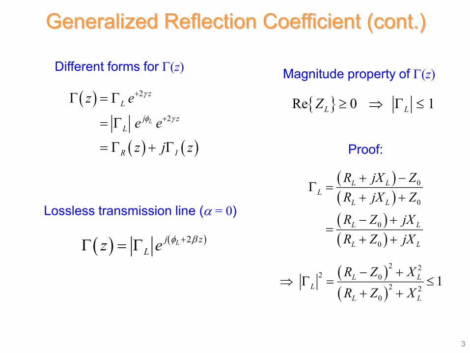
Generalized Reflection Coefficient (cont.)

{ }Re 0 1L LZ ≥ ⇒ Γ ≤

( )( )( )( )

0

0

0

0

L LL

L L

L L

L L

R jX ZR jX Z

R Z jXR Z jX

+ −Γ =

+ +

− +=

+ +

( )( )

2 22 0

2 20

1L LLL L

R Z XR Z X

− +⇒ Γ = ≤

+ +

Proof:

3

Different forms for Γ(z) Magnitude property of Γ(z)

Complex Γ Plane( )

( ) ( )( )

( )

( )

( )

2

2

2

2

L

L

R I

j zL

j zL

j dL

j dL

z

z j z

e

e

e

e

β

φ β

φ β

β

+

+

−

−

Γ = Γ

= Γ + Γ

= Γ

= Γ

= Γ

= Γ

Increasing d(moving towards

generator)

4

ReΓ

Im Γ

Lφ

LΓ

LΓ

2L dφ β−

Γ

Lossless line

z d= −d = distance from load

1

Note: Going λ/2 on the line

corresponds to going all the way around the Smith chart.

2 dβ

Clockwise movement!

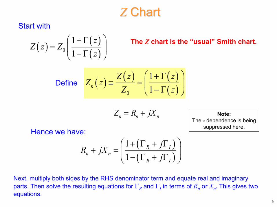
( ) ( )( )011

zZ z Z

z + Γ

= − Γ

( ) ( ) ( )( )011n

Z z zZ z

Z z + Γ

≡ = − Γ Define

n n nZ R jX= +

Hence we have:

Z Chart

( )( )

11

R In n

R I

jR jX

j + Γ + Γ

+ = − Γ + Γ

Next, multiply both sides by the RHS denominator term and equate real and imaginary parts. Then solve the resulting equations for ΓR and ΓI in terms of Rn or Xn. This gives two equations.

5

Note: The z dependence is being

suppressed here.

The Z chart is the “usual” Smith chart.

Start with

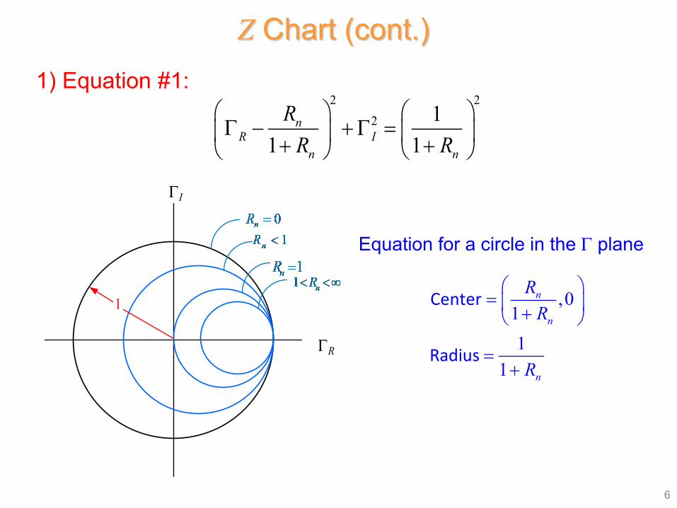
1) Equation #1:2 2

2 11 1

nR I

n n

RR R

Γ − + Γ = + +

Equation for a circle in the Γ plane

,011

1

n

n

n

RR

R

= +

=+

Center

Radius

Z Chart (cont.)

6

1

ΓR

ΓI

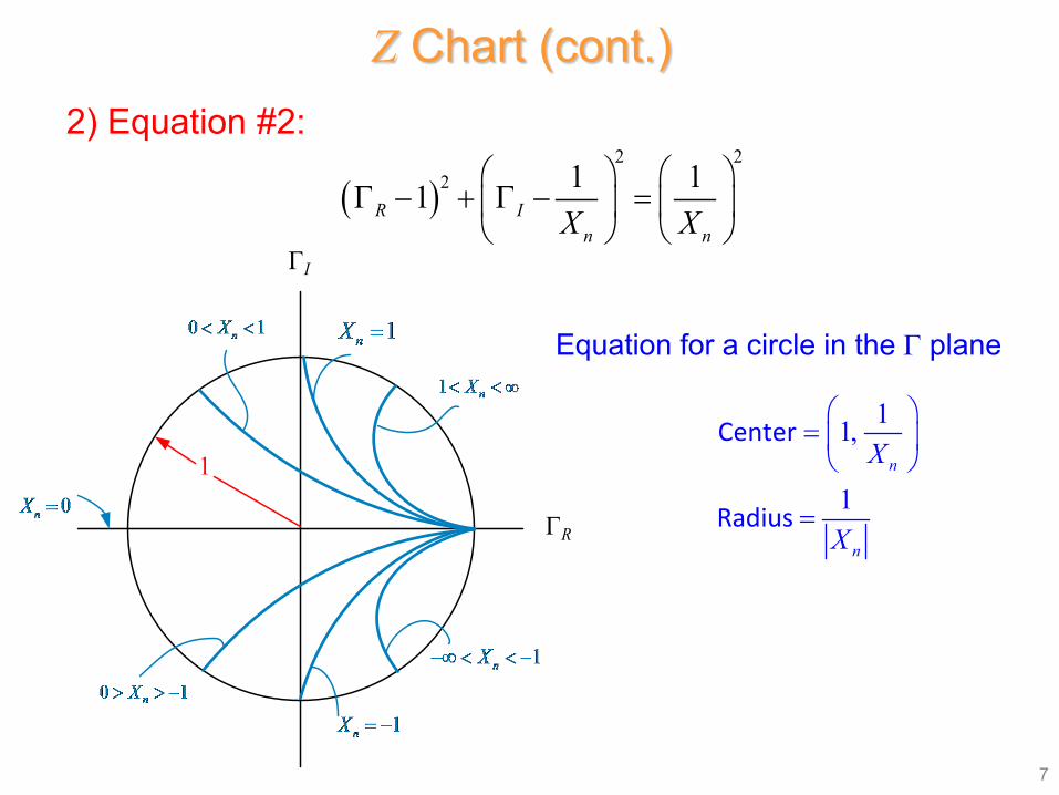
( )2 2

2 1 11R In nX X

Γ − + Γ − =

Equation for a circle in the Γ plane

11,

1n

n

X

X

=

=

Center

Radius

2) Equation #2:

7

1

ΓR

ΓI

Z Chart (cont.)

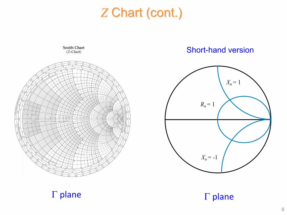
Short-hand version

8

Γ plane Γ plane

Rn = 1

Xn = 1

Xn = -1

Z Chart (cont.)

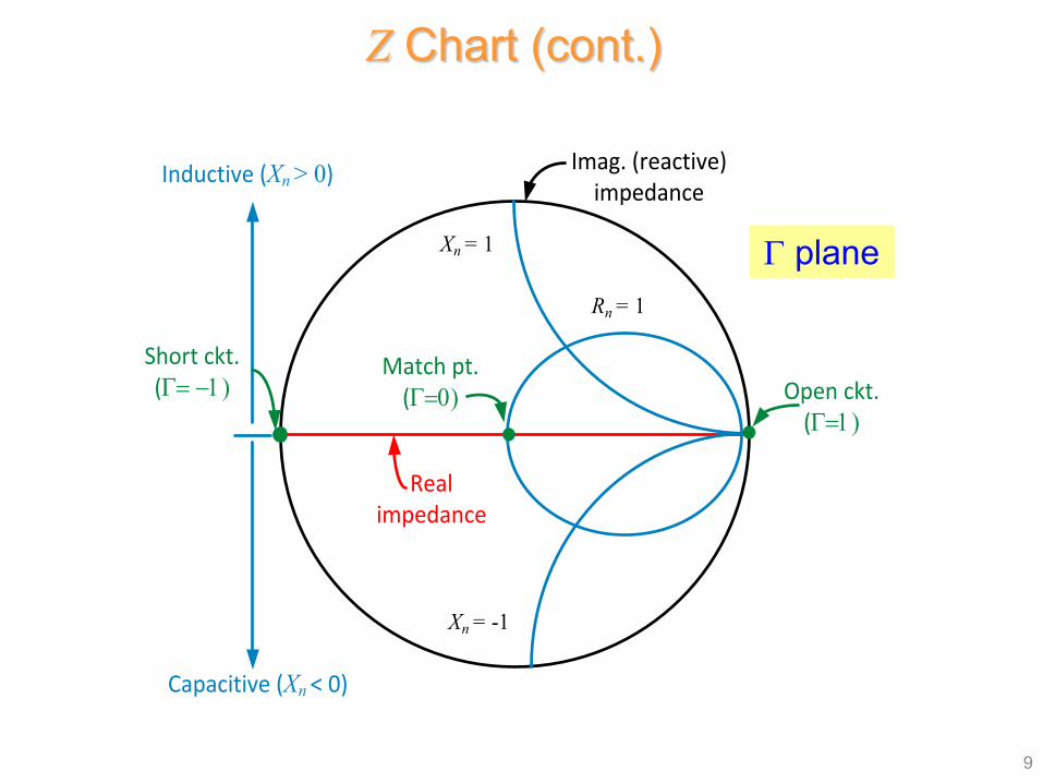
9

Open ckt. (Γ=1)

Imag. (reactive)impedance

Match pt. (Γ=0)

Realimpedance

Short ckt. (Γ= −1)

Inductive (Xn > 0)

Capacitive (Xn < 0)

Γ planeRn = 1

Xn = 1

Xn = -1

Γ plane

Z Chart (cont.)

Note: ( ) ( )( )( )0

11 11

zY z

Z z Z z − Γ

= = + Γ

( )( )( )( )0

11

zY

z + −Γ

= − −Γ

( ) ( ) ( )( )( )( ) ( ) ( )011n n n

zY zY z G z jB z

Y z + −Γ

⇒ ≡ = = + − −Γ

( )0 01 /Y Z≡

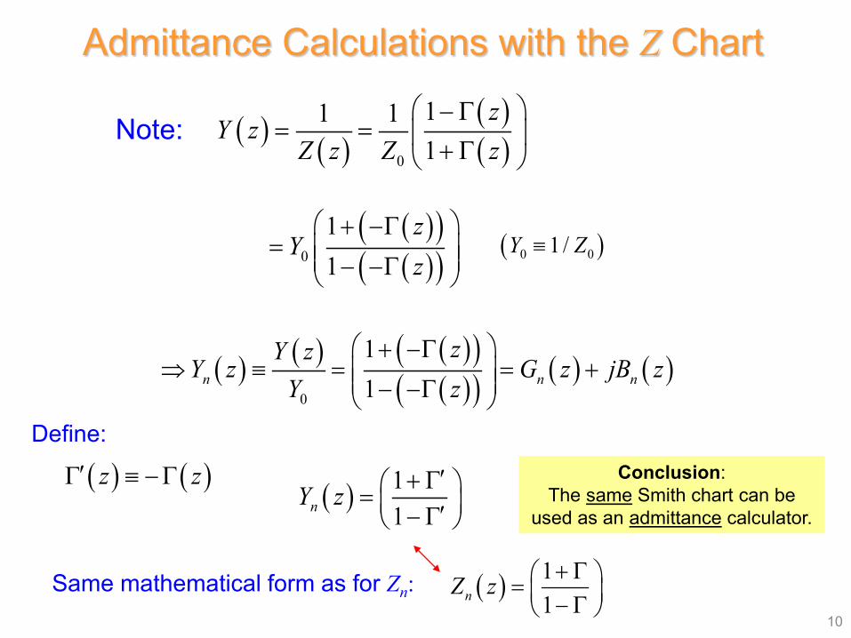
Admittance Calculations with the Z Chart

Define:

( ) ( )z z′Γ ≡ − Γ( ) 1

1nY z

′+ Γ = ′− Γ

Same mathematical form as for Zn:

Conclusion: The same Smith chart can be

used as an admittance calculator.

10

( ) 11n

Z z + Γ = − Γ

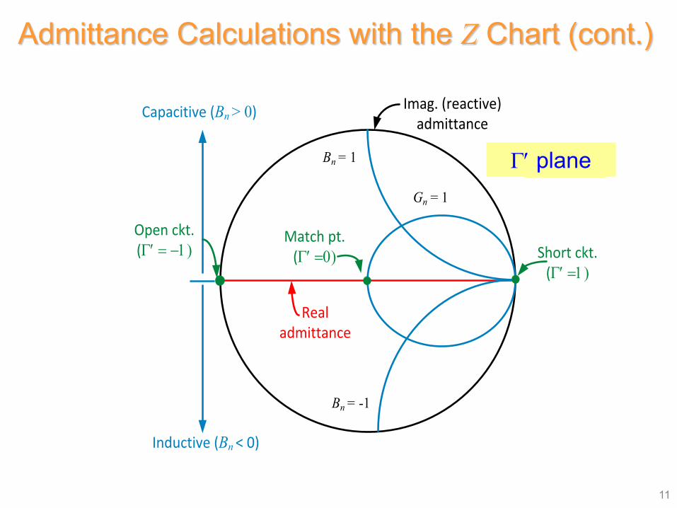
11

Short ckt. (Γ′ =1)

Imag. (reactive)admittance

Match pt. (Γ′ =0)

Realadmittance

Open ckt. (Γ′ = −1)

Capacitive (Bn > 0)

Inductive (Bn < 0)

Γ′ planeBn = 1

Bn = -1

Gn = 1

Γ′ plane

Admittance Calculations with the Z Chart (cont.)

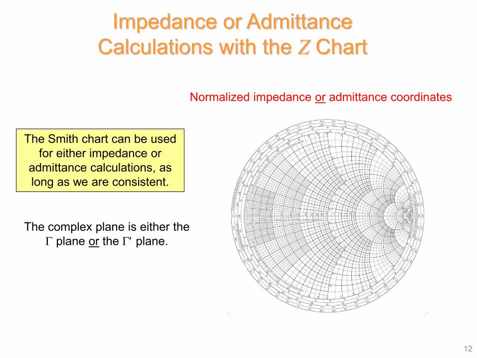
Impedance or Admittance Calculations with the Z Chart

12

The Smith chart can be used for either impedance or

admittance calculations, as long as we are consistent.

The complex plane is either the Γ plane or the Γ′ plane.

Normalized impedance or admittance coordinates

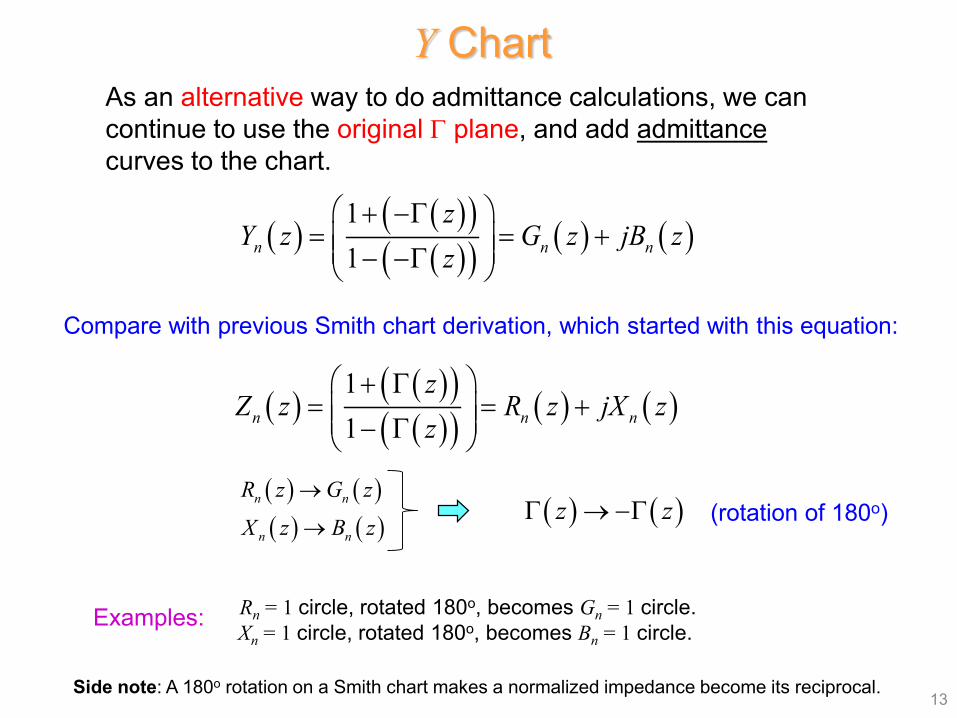
As an alternative way to do admittance calculations, we can continue to use the original Γ plane, and add admittancecurves to the chart.

( ) ( )( )( )( ) ( ) ( )11n n n

zY z G z jB z

z + −Γ

= = + − −Γ

Y Chart

( ) ( )( )( )( ) ( ) ( )11n n n

zZ z R z jX z

z + Γ

= = + − Γ

Compare with previous Smith chart derivation, which started with this equation:

Side note: A 180o rotation on a Smith chart makes a normalized impedance become its reciprocal. 13

Rn = 1 circle, rotated 180o, becomes Gn = 1 circle.Xn = 1 circle, rotated 180o, becomes Bn = 1 circle.

( ) ( )( ) ( )

n n

n n

R z G z

X z B z

→

→( ) ( )z zΓ → −Γ (rotation of 180o)

Examples:

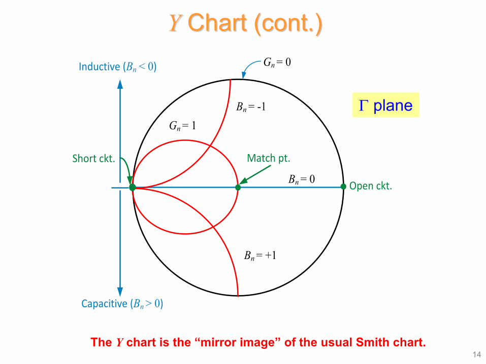
Y Chart (cont.)

14

Open ckt.

Match pt.

Gn = 0

Short ckt.

Inductive (Bn < 0)

Capacitive (Bn > 0)

Gn = 1

Bn = +1

Bn = -1

Bn = 0

Γ planeΓ plane

The Y chart is the “mirror image” of the usual Smith chart.

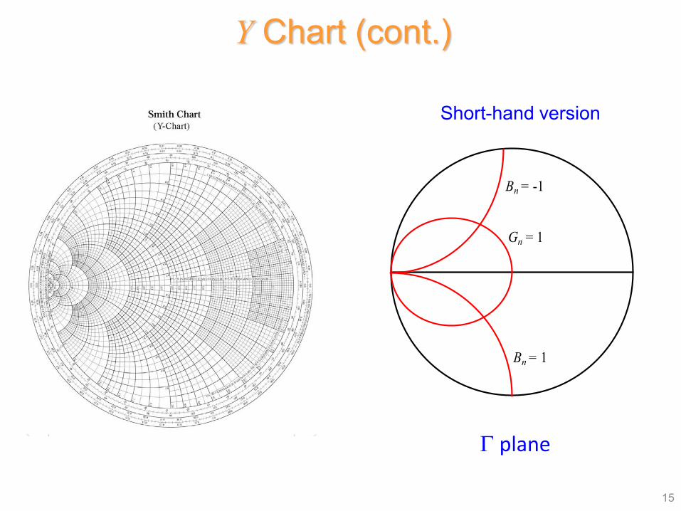
Short-hand version

Γ plane

15

Gn = 1

Bn = -1

Bn = 1

Y Chart (cont.)

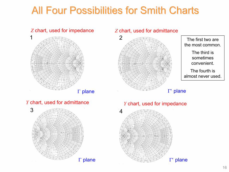
All Four Possibilities for Smith Charts

16

Z chart, used for admittance

Γ′ plane

Z chart, used for impedance

Γ plane

The first two are the most common.

The third is sometimes convenient.

The fourth is almost never used.

1 2

Γ′ plane

4Y chart, used for impedance

Γ plane

3Y chart, used for admittance

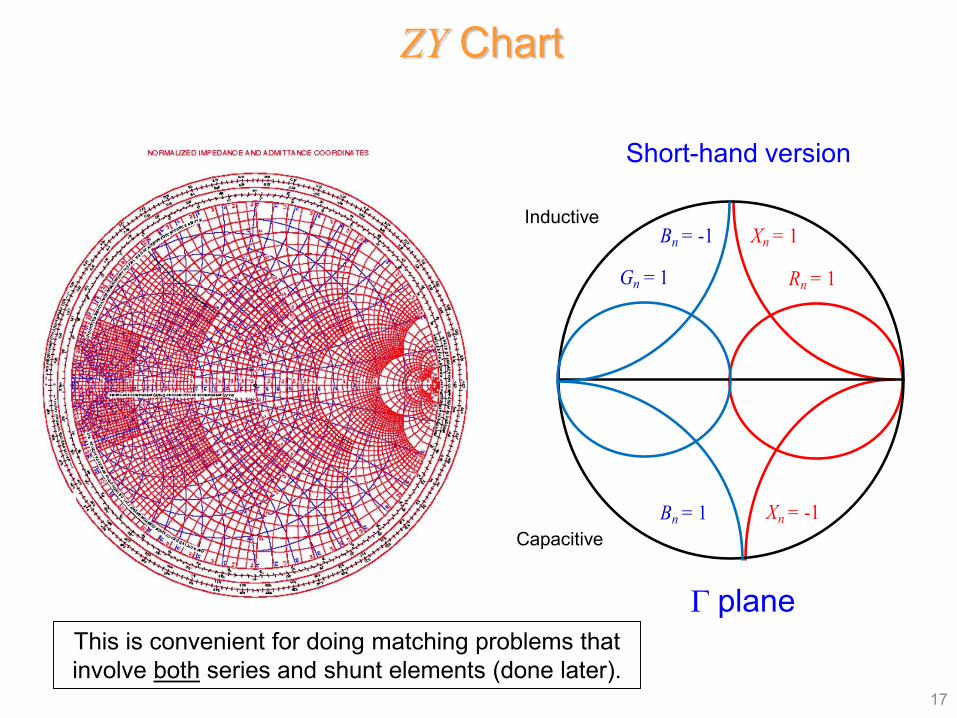
ZY Chart

17

This is convenient for doing matching problems that involve both series and shunt elements (done later).

Short-hand version

Γ plane

Gn = 1 Rn = 1

Xn = 1

Xn = -1

Bn = -1

Bn = 1

Inductive

Capacitive

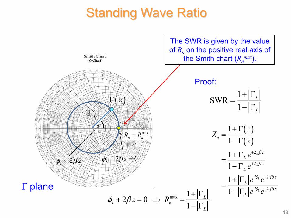
The SWR is given by the value of Rn on the positive real axis of

the Smith chart (Rnmax).

Standing Wave Ratio

Proof:1

SWR1

L

L

+ Γ=

− Γ

( )( )

2

2

2

2

11

1111

L

L

n

j zL

j zL

j j zL

j j zL

zZ

z

eee ee e

β

β

φ β

φ β

+

+

+

+

+ Γ=

− Γ

+ Γ=

− Γ

+ Γ=

− Γ

18

max 12 01

LL n

L

z Rφ β+ Γ

+ = ⇒ =− Γ

LΓ

maxn nR R=

2 0L zφ β+ =2L zφ β+

Γ plane

( )zΓ

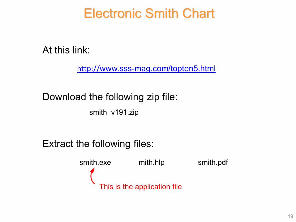
At this link:

http://www.sss-mag.com/topten5.html

Download the following zip file:smith_v191.zip

Extract the following files:

smith.exe mith.hlp smith.pdf

This is the application file

Electronic Smith Chart

19

http://www.sss-mag.com/topten5.html

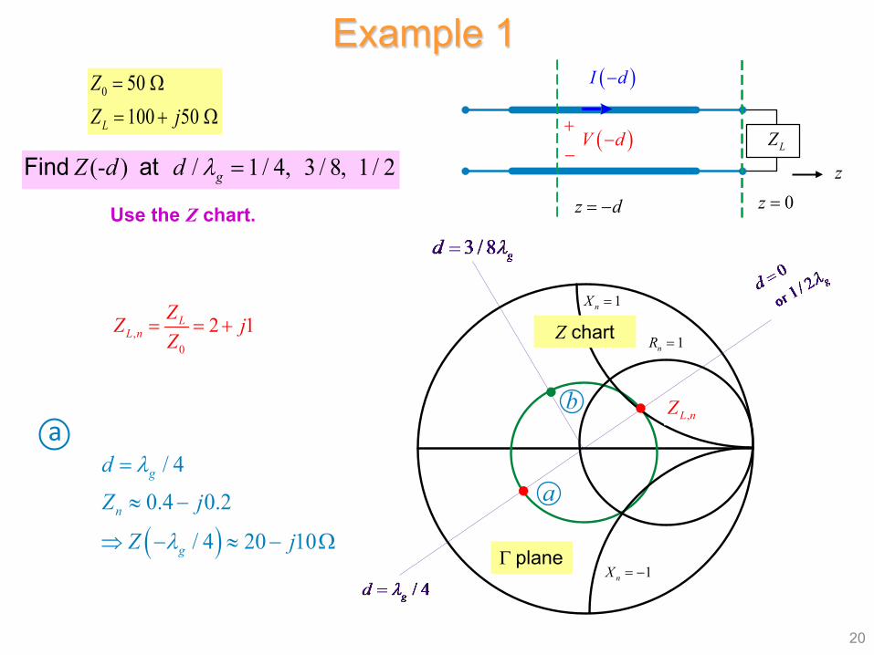
0 50100 50L

ZZ j

= Ω= + Ω

,0

2 1LL nZZ jZ

= = +

( )

/ 40.4 0.2

/ 4 20 10

g

n

g

dZ j

Z j

λ

λ

=

≈ −

⇒ − ≈ − Ω

Example 1

a

20

( )I d−

( )V d−

z d= −

+

−

0z =z

LZ(- ) / 1 / 4, 3 / 8, 1 / 2gZ d d λ =Find at

Use the Z chart.

a

b

Z chart

Γ plane

,L nZ

1nR =

1nX =

1nX = −

( )

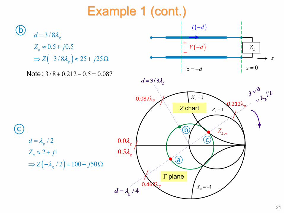
3 / 80.5 0.5

3 / 8 25 25

g

n

g

dZ j

Z j

λ

λ

=

≈ +

⇒ − ≈ + Ω

b

( )

/ 22 1

/ 2 100 50

g

n

g

dZ j

Z j

λ

λ

=

≈ +

⇒ − = + Ω

c

Example 1 (cont.)

21

3 / 8 0.212 0.5 0.087+ − =Note :

( )I d−

( )V d−

z d= −

+

−

0z =z

LZ

a

b

0.087λg

c0.5λg

0.462λg

0.212λgZ chart

Γ plane

0.0 gλ0.5 gλ

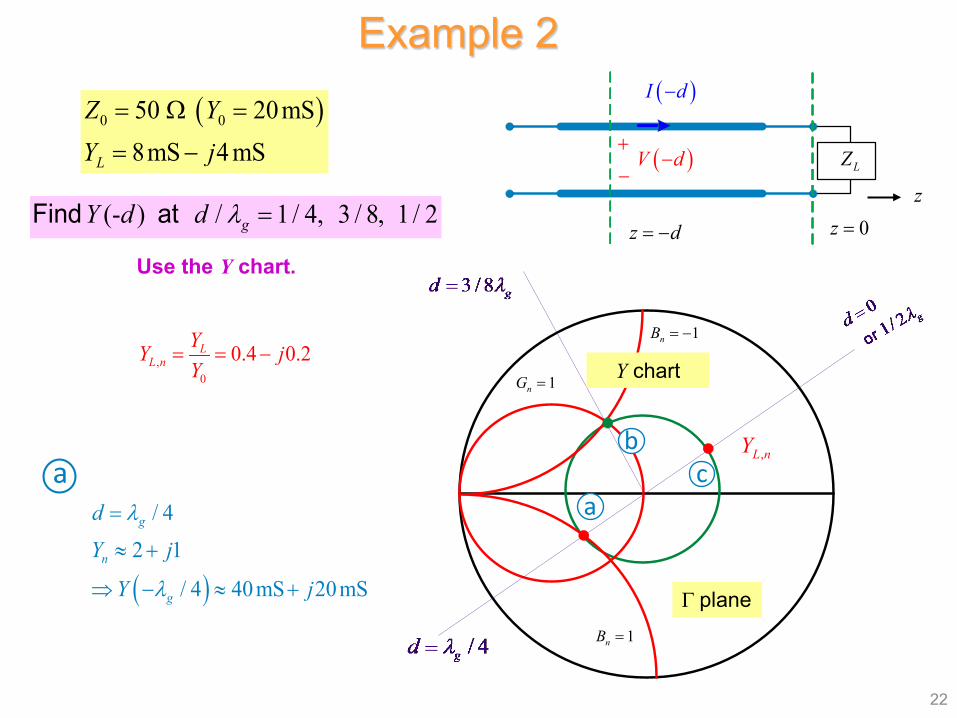
( )0 050 20mS8mS 4 mSL

Z YY j

= Ω =

= −

,0

0.4 0.2LL nYY jY

= = −

( )

/ 42 1

/ 4 40mS 20mS

g

n

g

dY j

Y j

λ

λ

=

≈ +

⇒ − ≈ +

Example 2

a

22

( )I d−

( )V d−

z d= −

+

−

0z =z

LZ

(- ) / 1 / 4, 3 / 8, 1 / 2gY d d λ =Find at

Use the Y chart.

a

bc

Y chart

Γ plane

,L nY

1nB = −

1nB =

1nG =

( )

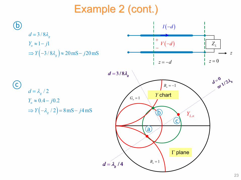
3 / 81 1

3 / 8 20mS 20mS

g

n

g

dY j

Y j

λ

λ

=

≈ −

⇒ − ≈ −

( )

/ 20.4 0.2

/ 2 8mS 4mS

g

n

g

dY j

Y j

λ

λ

=

≈ −

⇒ − = −

Example 2 (cont.) b

c

23

( )I d−

( )V d−

z d= −

+

−

0z =z

LZ

a

bc

Y chart

Γ plane

,L nY

1nB = −

1nB =

1nG =

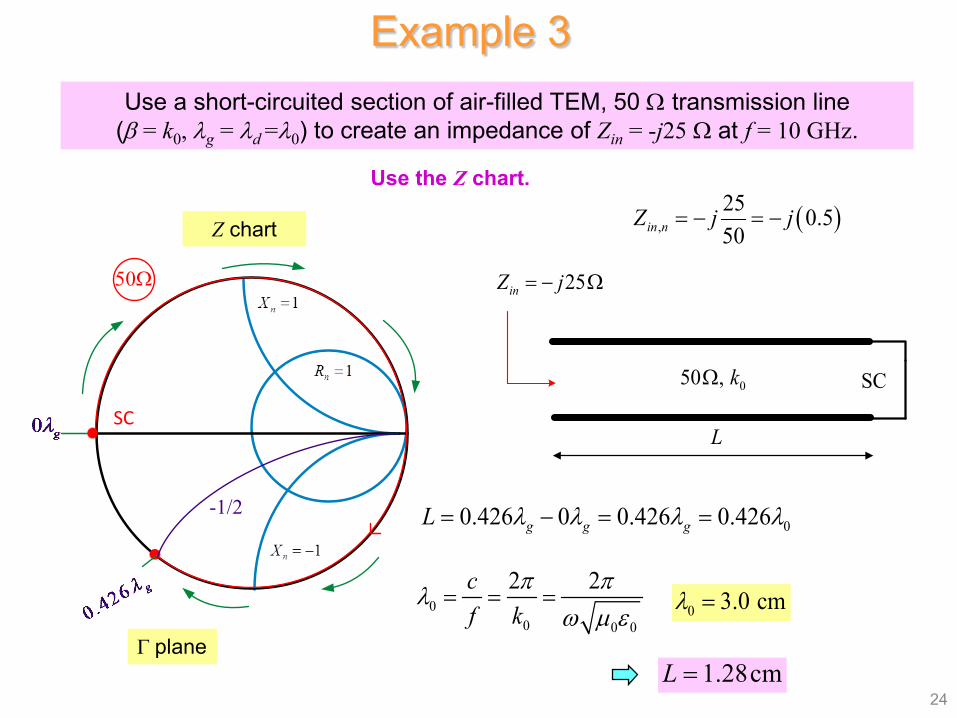
Use a short-circuited section of air-filled TEM, 50 Ω transmission line(β = k0, λg = λd =λ0) to create an impedance of Zin = -j25 Ω at f = 10 GHz.

( ),25 0.550in n

Z j j= − = −

00.426 0 0.426 0.426g g gL λ λ λ λ= − = =

Example 3

24

00 0 0

2 2cf k

π πλω µ ε

= = =0 3.0 cmλ =

25inZ j= − Ω

050 , kΩ SC

L

1.28cmL =

Z chart

Γ plane

SC

-1/2

50Ω

Use the Z chart.

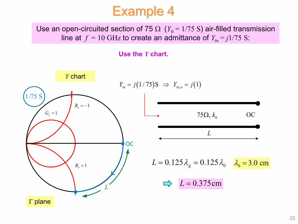
Use an open-circuited section of 75 Ω (Y0 = 1/75 S) air-filled transmission line at f = 10 GHz to create an admittance of Yin = j1/75 S:

0.375cmL =

Example 4

25

00.125 0.125gL λ λ= = 0 3.0 cmλ =

( ) ( ),1 / 75 S 1in in nY j Y j= ⇒ =

075 , kΩ OC

L

Y chart

Γ plane

j1

1/75 S

OC

L

1nB = −

1nB =

Use the Y chart.

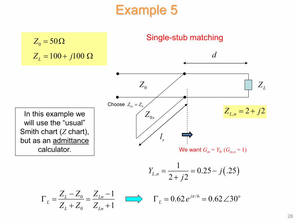
Example 5

0 50Z = Ω

100 100LZ j= + Ω

( ),1 0.25 .25

2 2L nY j

j= = −

+

/6 o0.62 0.62 30jL eπΓ = = ∠0

0

11

L LnL

L Ln

Z Z ZZ Z Z

− −Γ = =

+ +26

In this example we will use the “usual”

Smith chart (Z chart), but as an admittance

calculator.

Single-stub matching

, 2 2L nZ j= +

0Z

0sZ

LZ

d

slWe want Gin = Y0 (Gin,n = 1)

0 0sZ Z=Choose

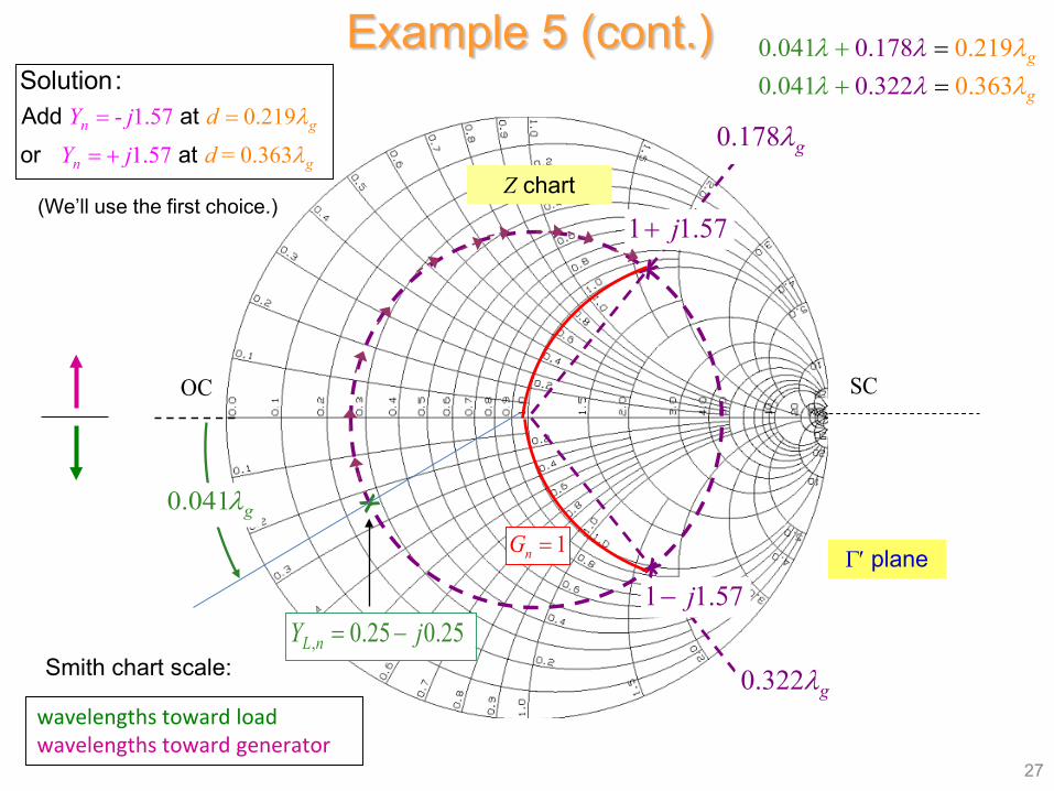
Example 5 (cont.)

0.178 gλ

, 0.25 0.25L nY j= −

1 1.57j+

1 1.57j−

0.322 gλ

0.041 gλ

0.219- 1.57

= 1.57 0.363gn

gn

dY

Y j d

j λ

λ

= =

= +

Add ator at

Solution:0.170 0.2.0 981 14 gλ λλ =+0.320 0.3.0 321 64 gλ λλ =+

wavelengths toward loadwavelengths toward generator

Smith chart scale:

Z chart

27

Γ′ plane

(We’ll use the first choice.)

SCOC

1nG =

Example 5 (cont.)

( )( )

( )

( )

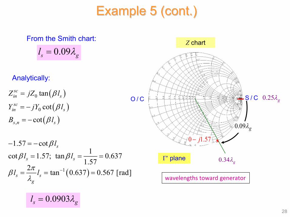
0

0

,

1

tan

cot

cot

1.57 cot1cot 1.57; tan 0.637

1.572 tan 0.637 0.567 [rad]

scin s

scin s

s n s

s

s s

s sg

Z jZ l

Y jY l

B l

l

l l

l l

β

β

β

β

β βπβ

λ−

=

= −

= −

− = −

= = =

= = =

0.09s gl λ=From the Smith chart:

0.0903s gl λ=

Analytically:

28

S / C

0 1.57j−

0.09 gλ

O / C

Z chart

Γ′ plane

0.25 gλ

0.34 gλ

wavelengths toward generator

Example 5 (cont.)

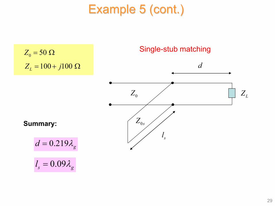
0 50Z = Ω

100 100LZ j= + Ω

29

0Z

0sZ

LZ

d

sl

Single-stub matching

0.09s gl λ=

0.219 gd λ=

Summary:

Slide Number 1Slide Number 2Slide Number 3Slide Number 4Slide Number 5Slide Number 6Slide Number 7Slide Number 8Slide Number 9Slide Number 10Slide Number 11Slide Number 12Slide Number 13Slide Number 14Slide Number 15Slide Number 16Slide Number 17Slide Number 18Slide Number 19Slide Number 20Slide Number 21Slide Number 22Slide Number 23Slide Number 24Slide Number 25Slide Number 26Slide Number 27Slide Number 28Slide Number 29