A MATLAB toolbox for optimizing splines

Wannes Van Loock, Goele Pipeleers and Jan SweversKU Leuven, BE-3001 Leuven, Belgium

Depertment of Mechanical Engineering, Division PMAWannes.VanLoock@kuleuven.be

1 Introduction

This work presents a new MATLAB toolbox for modelingand solving optimization problems of the following form

minimizex

f (x)

subject to h(x,θ)≥ 0,∀θ ∈Θ

where x are the coefficients of a (polynomial) spline

s(x,θ) = ∑α

xα bα(θ),

with basis bα and labeled by the (multi-)index α .

The main challenge when solving these problems lies intransforming the constraints that should hold for infinitelymany values of θ , so-called semi-infinite constraints, to a(conservative) finite set of constraint. For spline repre-sentable h(x, ·), this toolbox implements an efficient novelrelaxation scheme based on the partition of unity of the ba-sis functions and using knot insertion.

Spline solutions of the problem can be interpreted as an ap-proximation to the solution of the more general infinite di-mensional problem in which a function s(·) is searched forwithout preset parameterization. For these problems, splinesare a particularly interesting parameterization as it can beshown that splines are a good approximation of smoothfunctions [1]. The toolbox therefore enables solving manypractical that arise in engineering, physics, economics, andso on. In control engineering applications, one can thinkof optimal control problems, explicit model predictive con-trollers, the design of H∞/H2 gain scheduling controllersand combined structure and control design. A spline

0 1 2 3 4

2

4

6

θ

x 1(θ

)+

2x2(

θ)

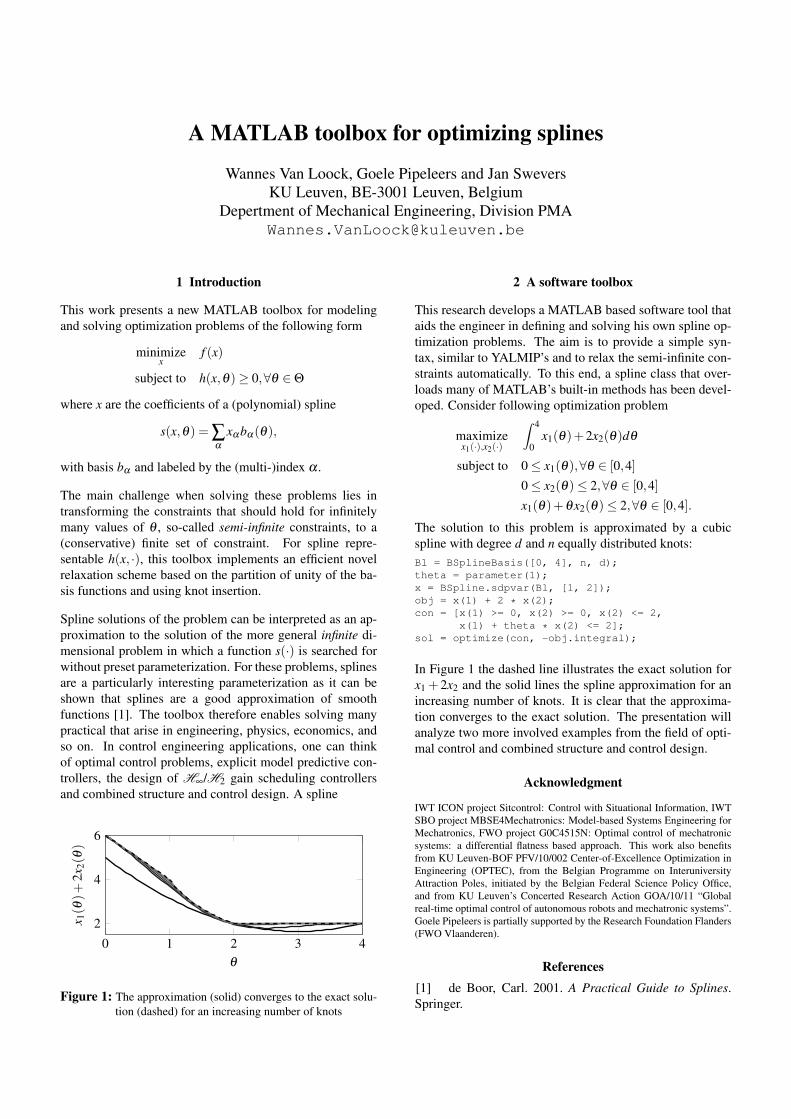
Figure 1: The approximation (solid) converges to the exact solu-tion (dashed) for an increasing number of knots

2 A software toolbox

This research develops a MATLAB based software tool thataids the engineer in defining and solving his own spline op-timization problems. The aim is to provide a simple syn-tax, similar to YALMIP’s and to relax the semi-infinite con-straints automatically. To this end, a spline class that over-loads many of MATLAB’s built-in methods has been devel-oped. Consider following optimization problem

maximizex1(·),x2(·)

∫ 4

0x1(θ)+2x2(θ)dθ

subject to 0≤ x1(θ),∀θ ∈ [0,4]0≤ x2(θ)≤ 2,∀θ ∈ [0,4]x1(θ)+θx2(θ)≤ 2,∀θ ∈ [0,4].

The solution to this problem is approximated by a cubicspline with degree d and n equally distributed knots:Bl = BSplineBasis([0, 4], n, d);theta = parameter(1);x = BSpline.sdpvar(Bl, [1, 2]);obj = x(1) + 2 * x(2);con = [x(1) >= 0, x(2) >= 0, x(2) <= 2,

x(1) + theta * x(2) <= 2];sol = optimize(con, -obj.integral);

In Figure 1 the dashed line illustrates the exact solution forx1 + 2x2 and the solid lines the spline approximation for anincreasing number of knots. It is clear that the approxima-tion converges to the exact solution. The presentation willanalyze two more involved examples from the field of opti-mal control and combined structure and control design.

Acknowledgment

IWT ICON project Sitcontrol: Control with Situational Information, IWTSBO project MBSE4Mechatronics: Model-based Systems Engineering forMechatronics, FWO project G0C4515N: Optimal control of mechatronicsystems: a differential flatness based approach. This work also benefitsfrom KU Leuven-BOF PFV/10/002 Center-of-Excellence Optimization inEngineering (OPTEC), from the Belgian Programme on InteruniversityAttraction Poles, initiated by the Belgian Federal Science Policy Office,and from KU Leuven’s Concerted Research Action GOA/10/11 “Globalreal-time optimal control of autonomous robots and mechatronic systems”.Goele Pipeleers is partially supported by the Research Foundation Flanders(FWO Vlaanderen).

References[1] de Boor, Carl. 2001. A Practical Guide to Splines.Springer.