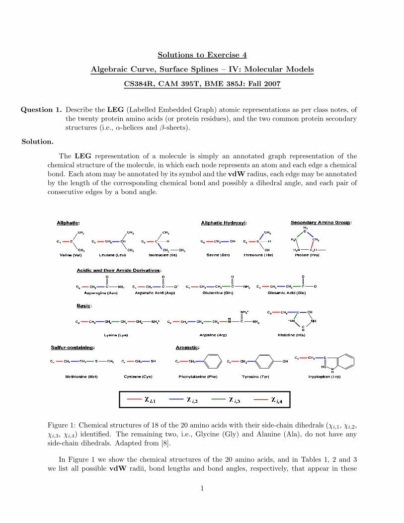
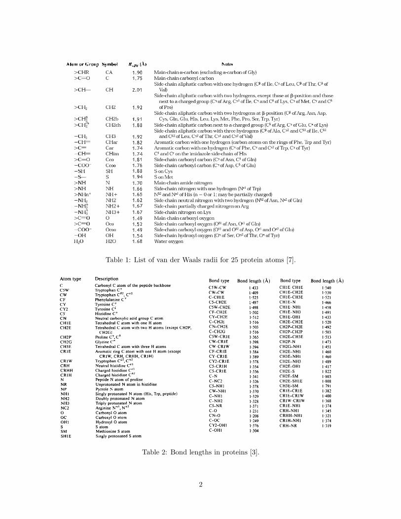
Solutions to Exercise 4

Algebraic Curve, Surface Splines – IV: Molecular Models

CS384R, CAM 395T, BME 385J: Fall 2007

Question 1. Describe the LEG (Labelled Embedded Graph) atomic representations as per class notes, ofthe twenty protein amino acids (or protein residues), and the two common protein secondarystructures (i.e., α-helices and β-sheets).

Solution.

The LEG representation of a molecule is simply an annotated graph representation of thechemical structure of the molecule, in which each node represents an atom and each edge a chemicalbond. Each atom may be annotated by its symbol and the vdW radius, each edge may be annotatedby the length of the corresponding chemical bond and possibly a dihedral angle, and each pair ofconsecutive edges by a bond angle.

����� ����� �� ����� ��� ������� ��� ��� ��� ���� ����� ��� ��� �� �������� ����� � �� �������

����� ��� � ��� ����� �������� ���� ����� ��� ����� ��� ����� ����� ��� ���

����� �� ��� ������ ��� ������ ���������� ������ ��� ������� �������� ���������� ������� ������� �� ����� ���������� ����� ���������� ��������� ���� ���� ��������� ���� ���� ������� ��� ����� ���� ���� ��� �!����� ��� ����� ���� ���� ��� �!��"�!��"�!����

���#�����#��$$���������%���������%�� ����������������

&'()*+ ,&'(- .+/0)*+ ,.+/- 123(+/0)*+ ,1(+- 4+5)*+ ,4+5- 675+3*)*+ ,675- 853()*+ ,853-92:'5';)*+ ,92*- 92:'5'<)0 90)= ,92:- >(/<'?)*+ ,>(*- >(/<'?)0 90)= ,>(/-

.@2)*+ ,.@2- 95;)*)*+ ,95;- A)2<)=)*+ ,A)2-B+<7)3*)*+ ,B+<- C@2<+)*+ ,C@2- 87+*@('('*)*+ ,87+- 6@532)*+ ,6@5- 65@:<3:7'* ,65:-D EFG D EFH D EFI D EFJ

Figure 1: Chemical structures of 18 of the 20 amino acids with their side-chain dihedrals (χi,1, χi,2,χi,3, χi,4) identified. The remaining two, i.e., Glycine (Gly) and Alanine (Ala), do not have anyside-chain dihedrals. Adapted from [8].

In Figure 1 we show the chemical structures of the 20 amino acids, and in Tables 1, 2 and 3we list all possible vdW radii, bond lengths and bond angles, respectively, that appear in these

1

KLMNKLOPQLNKKLMQKLMKKLRRKLMQKLRQKLOSKLOSKLRKKLOTKLRRKLMSKLONKLTTKLTPKLTQKLTOKLTOKLSMKLPQKLSMKLPSKLTR

UVWX YZ[\]^_ ^` a`^bc de_f^g h^]ij

Table 1: List of van der Waals radii for 25 protein atoms [7].

Table 2: Bond lengths in proteins [3].

2

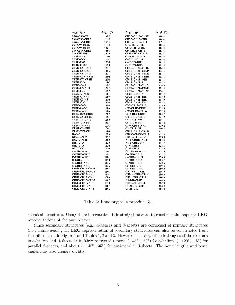
Table 3: Bond angles in proteins [3].

chemical structures. Using these information, it is straight-forward to construct the required LEGrepresentations of the amino acids.

Since secondary structures (e.g., α-helices and β-sheets) are composed of primary structures(i.e., amino acids), the LEG representation of secondary structures can also be constructed fromthe information in Figure 1 and Tables 1, 2 and 3. However, the (φ,ψ) dihedral angles of the residuesin α-helices and β-sheets lie in fairly restricted ranges: (−45◦,−60◦) for α-helices, (−120◦, 115◦) forparallel β-sheets, and about (−140◦, 135◦) for anti-parallel β-sheets. The bond lengths and bondangles may also change slightly.

3

Question 2. Given a LEG representation of a protein (created from the PDB), describe an algorithmto detect and output the LEG representations of all α-helices and β-sheets in that protein.Your algorithm should be able to distinguish between parallel and anti-parallel β-sheets.

Solution.

We will use geometric properties of α-helices and β-sheets in order to extract them from theLEG representation L of the given protein P .

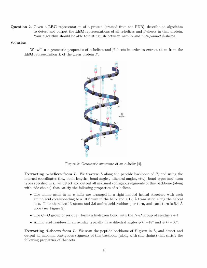
Figure 2: Geometric structure of an α-helix [4].

Extracting α-helices from L. We traverse L along the peptide backbone of P , and using theinternal coordinates (i.e., bond lengths, bond angles, dihedral angles, etc.), bond types and atomtypes specified in L, we detect and output all maximal contiguous segments of this backbone (alongwith side chains) that satisfy the following properties of α-helices.

• The amino acids in an α-helix are arranged in a right-handed helical structure with eachamino acid corresponding to a 100◦ turn in the helix and a 1.5 A translation along the helicalaxis. Thus there are 13 atoms and 3.6 amino acid residues per turn, and each turn is 5.4 Awide (see Figure 2).

• The C=O group of residue i forms a hydrogen bond with the N -H group of residue i+ 4.

• Amino acid residues in an α-helix typically have dihedral angles φ ≈ −45◦ and ψ ≈ −60◦.

Extracting β-sheets from L. We scan the peptide backbone of P given in L, and detect andoutput all maximal contiguous segments of this backbone (along with side chains) that satisfy thefollowing properties of β-sheets.

4

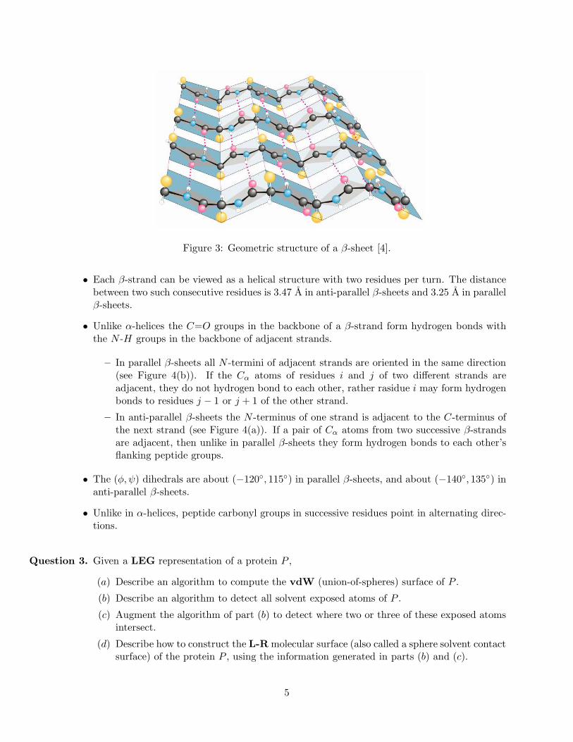
Figure 3: Geometric structure of a β-sheet [4].

• Each β-strand can be viewed as a helical structure with two residues per turn. The distancebetween two such consecutive residues is 3.47 A in anti-parallel β-sheets and 3.25 A in parallelβ-sheets.

• Unlike α-helices the C=O groups in the backbone of a β-strand form hydrogen bonds withthe N -H groups in the backbone of adjacent strands.

– In parallel β-sheets all N -termini of adjacent strands are oriented in the same direction(see Figure 4(b)). If the Cα atoms of residues i and j of two different strands areadjacent, they do not hydrogen bond to each other, rather rasidue i may form hydrogenbonds to residues j − 1 or j + 1 of the other strand.

– In anti-parallel β-sheets the N -terminus of one strand is adjacent to the C-terminus ofthe next strand (see Figure 4(a)). If a pair of Cα atoms from two successive β-strandsare adjacent, then unlike in parallel β-sheets they form hydrogen bonds to each other’sflanking peptide groups.

• The (φ,ψ) dihedrals are about (−120◦, 115◦) in parallel β-sheets, and about (−140◦, 135◦) inanti-parallel β-sheets.

• Unlike in α-helices, peptide carbonyl groups in successive residues point in alternating direc-tions.

Question 3. Given a LEG representation of a protein P ,

(a) Describe an algorithm to compute the vdW (union-of-spheres) surface of P .

(b) Describe an algorithm to detect all solvent exposed atoms of P .

(c) Augment the algorithm of part (b) to detect where two or three of these exposed atomsintersect.

(d) Describe how to construct the L-R molecular surface (also called a sphere solvent contactsurface) of the protein P , using the information generated in parts (b) and (c).

5

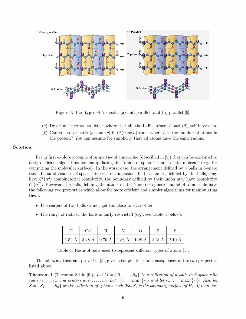
Figure 4: Two types of β-sheets: (a) anti-parallel, and (b) parallel [6].

(e) Describe a method to detect where if at all, the L-R surface of part (d), self intersects.

(f) Can you solve parts (b) and (c) in O (n log n) time, where n is the number of atoms inthe protein? You can assume for simplicity that all atoms have the same radius.

Solution.

Let us first explore a couple of properties of a moleclue (described in [5]) that can be exploited todesign efficient algorithms for manipulating the “union-of-sphere” model of the molecule (e.g., forcomputing the molecular surface). In the worst case, the arrangement defined by n balls in 3-space(i.e., the subdivision of 3-space into cells of dimensions 0, 1, 2, and 3, defined by the balls) mayhave O

(

n3)

combinatorial complexity, the boundary defined by their union may have complexityO

(

n2)

. However, the balls defining the atoms in the “union-of-sphere” model of a molecule havethe following two proporties which allow for more efficient and simpler algorithms for manipulatingthem:

• The centers of two balls cannot get too close to each other.

• The range of radii of the balls is fairly restricted (e.g., see Table 4 below).

C Cal H N O P S

1.52 A 3.48 A 0.70 A 1.36 A 1.28 A 2.18 A 2.10 A

Table 4: Radii of balls used to represent different types of atoms [5].

The following theorem, proved in [5], gives a couple of useful consequences of the two propertieslisted above.

Theorem 1 (Theorem 2.1 in [5]). Let M = {B1, . . . , Bn} be a collection of n balls in 3-space withradii r1, . . . , rn and centers at c1, . . . , cn. Let rmin = mini {ri} and let rmax = maxi {ri}. Also letS = {S1, . . . , Sn} be the collection of spheres such that Si is the boundary surface of Bi. If there are

6

positive constants k, ρ such that rmax

rmin

< k and for each Bi the ball with radius ρ · ri and concentricwith Bi does not contain the center of any other ball in M (besides ci), then:

(i) For each Bi ∈ M , the maximum number of balls in M that intersect it is bounded by aconstant.

(ii) The maximum combinatorial complexity of the boundary of the union of the balls in M isO (n).

Table 5 lists the values of k, ρ and the maximum and average number of balls intersecting anygiven ball in various molecules [5]. As the table shows, k is quite small and ρ is quite close to 1,resulting in a small number of insersections per ball.

molecule k ρmaximum number of balls

intersecting a given ball

avgerage number of balls

intersecting a given ball

caffine 2.17 0.71 10 4.5

acetyl 3.11 0.67 16 5.4

crambin 1.64 0.78 10 5.5

felix 1.64 0.81 9 4.9

SuperOxide Dismutase 1.95 0.76 16 5.5

Table 5: Values of k, ρ and the maximum and average number of balls intersecting a single ball invarious molecules [5].

Given a “union-of-ball” representation of a molecule, Theorem 1 can now be used to design anefficient data structure that can answer insersection queries with either a point or with a ball whoseradius is bounded by a rmax. We will use this data structure in parts 3(a) – 3(f).

An Efficient Intersection Query Data Structure (from [5]). Let M be the set of n ballsas defined in Theorem 1. We subdivide the entire 3-space into axis-parallel cubes of size 2rmax ×2rmax × 2rmax each. For each B ∈M , we compute the grid cubes that B intersects. Let C be theset of non-empty grid cubes. Since each ball can intersect at most 8 grid cubes, the size of C isbounded by O (n). Also observe that according to Theorem 1, each cube can be intersected by atmost a constant number of balls. We store the cubes in C in a balanced binary search tree orderedlexicographically by the bottom-left-front vertices of the cubes. With each cube we store the listof O (1) balls of M that intersects it.

Now given a query ball Q, we compute all (at most 8) grid cubes it intersects, and search foreach of these cubes in the binary search tree. For each such cube that exists in the search tree, wecheck the balls stored in it for intersection with Q. Each search will take O (log n) time, and thetotal number of balls tested will be O (1). Hence, we have the following theorem.

Theorem 2 (Theorem 3.1 in [5]). Given a collection M of n balls as defined in Theorem 1, onecan construct a data structure using O (n) space and O (n log n) preprocessing time, to answerintersection queries for balls whose radii are not greater than rmax, in time O (log n).

7

klk mkn opqrpsttuvwx ooyrzs kk{ mlnt|tv}x~ ���� �� � ���� ��

������������ �������

���������� �¡¢ ¡¢

£

¤¥¡¦

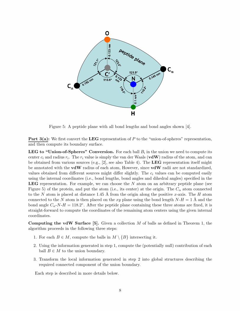
Figure 5: A peptide plane with all bond lengths and bond angles shown [4].

Part 3(a): We first convert the LEG representation of P to the “union-of-spheres” representation,and then compute its boundary surface.

LEG to “Union-of-Spheres” Conversion. For each ball Bi in the union we need to compute itscenter ci and radius ri. The ri value is simply the van der Waals (vdW) radius of the atom, and canbe obtained from various sources (e.g., [2], see also Table 4). The LEG representation itself mightbe annotated with the vdW radius of each atom, However, since vdW radii are not standardized,values obtained from different sources might differ slightly. The ci values can be computed easilyusing the internal coordinates (i.e., bond lengths, bond angles and dihedral angles) specified in theLEG representation. For example, we can choose the N atom on an arbitrary peptide plane (seeFigure 5) of the protein, and put the atom (i.e., its center) at the origin. The Cα atom connectedto the N atom is placed at distance 1.45 A from the origin along the positive x-axis. The H atomconnected to the N atom is then placed on the xy plane using the bond length N -H = 1 A and thebond angle Cα-N -H = 118.2◦. After the peptide plane containing these three atoms are fixed, it isstraight-forward to compute the coordinates of the remaining atom centers using the given internalcoordinates.

Computing the vdW Surface [5]. Given a collection M of balls as defined in Theorem 1, thealgorithm proceeds in the following three steps:

1. For each B ∈M , compute the balls in M \ {B} intersecting it.

2. Using the information generated in step 1, compute the (potentially null) contribution of eachball B ∈M to the union boundary.

3. Transform the local information generated in step 2 into global structures describing therequired connected component of the union boundary.

Each step is described in more details below.

8

Step 1: We use the intersection query data structure described earlier (see Theorem 2). Each in-tersection query takes O (log n) time, and hence the total cost of this step is O (n log n).

Step 2: Let Bi be a ball, and we want to compute its contribution to the union boundary. Weknow from Theorem 1 that at most a constant number of other balls intersect Bi. Let Bj be sucha ball, if any. We consider the following three cases:

(i) If Bj fully contains Bi, we stop processing Bi as it cannot contribute to the union boundary.

(ii) If Bi fully contains Bj , we simply ignore Bj.

(iii) If neither of the two cases above holds, we compute the intersection between Si and Sj, whichis a circle Cij on Si (and Sj). This circle splits Si into two parts: one part is completelycontained within Sj and hence cannot contribute to the union boundary, and the other partwhich is called the free part of Si, may actually appear on the union boundary.

After the process above is repeated for every ball intersecting Bi, we get a collection of circles onSi. These circles form a 2D arrangement Ai on Si. A face of Ai belongs to the union boundary iffit is on the free part defined by each such circle. Since the number of such circles is O (1), Ai canbe computed in O (1) time using brute force. Within the same bound we can mark each face onAi as free or not free. A free face is guaranteed to appear on the union boundary. Since the aboveprocedure for Bi takes O (1) time, the total time complexity of this step is O (n).

Step 3: In this step, the outer connected component of the union bounadry of M is representedusing a graph data structure. In order to do so, each arrangement Ai is augmented slightly asfollows. If Ai is the whole sphere Si, it is split into two parts using some circle. Next, if a boundarycomponent of Ai is a simple circle C, then C is split into two arcs by adding two new vertices. IfC belongs to two arangements Ai and Aj , the same two vertices are added to both arrangements.Finally, if a free face of Ai contains holes, the face is split into (sub)faces by adding extra arcs sothat none of (sub)faces contains any holes in it. All these additions are made canonical by fixing adirection d, and adding all extra edges along great circles that are intersections of Si with planesparallel to the direction d. This step can easily be performed in O (n) time, and after this step theunion boundary will consist of only simple faces that are bounded by at least two edges, and eachedge will be shared by exactly two faces (assuming general position).

Now we compute the vdW surface (i.e., the outer union boundary) of M and store it as agraph G = (V,E) (which is initially empty) as follows. First, we find the ball Bmax ∈ M withthe point having the largest z-coordinate. Let fmax be the face of Bmax that contains this point.Then clearly fmax belongs to the outer union boundary of M . Now starting from this face fmax wetraverse the entire connected component containing fmax using depth-first search. Each free facef we encounter during this traversal will be made a vertex vf ∈ V , and each arc shared by twosuch faces f1 and f2 will be made an edge (vf1

, vf2) ∈ E. Everytime we encounter a free face f

which has not been visited before, we determine its boundary (i.e., the edges bounding this face),which can be done in O (1) time. For each such edge e of f , we can find the face f ′ that shares ein O (1) time. If f ′ is a free face and has not been visited before, we recursively visit f ′. After wehave visited each free face reachable from fmax once, G contains the vdW surface of M . Clearly,this traversal takes O (1) time.

Hence, the following theorem follows.

Theorem 3 (Theorem 4.1 in [5]). The vdW surface of the union of a connected collection of ballsas defined in Theorem 1 can be computed in O (n log n) time and O (n) space.

9

Part 3(b): We increase the radius of each atom in P by rs, where rs is the radius of a solventatom. Clearly, the collection of these enlarged atoms still satisfies the requirements of Theorem 1,and the theorem holds. Hence, we can find all atoms in this collection that contribute to the outerunion boundary in O (n log n) time and O (n) space using the same algorithm as in part 3(a).

Part 3(c): The algorithm in part 3(b) already constructs the intersection query data structuredescribed earlier for the set of enlarged atoms in P . If P contains n atoms, this construction takesO (n log n) time and uses O (n) space. The algorithm also identifies all solvent exposed atoms.Now, for any ball Bi representing a solvent exposed atom in P , we can find the set Ti of O (1)other solvent exposed atoms that intersects it in O (log n) time. Since the size of the set Ti ∪ {Bi}is bounded by a constant, we can detect in O (1) time where two or three of the atoms in this setintersect. We can identify all such intersections in O (n log n) time and O (n) space by using thesame process as above for each solvent exposed atoms in P .§¨©ª«¬ ­®¯«°±§²³ ®²´§¯ ´¨°¨±µ²³ ®²´§¯

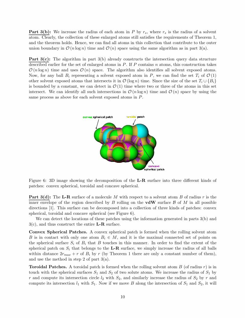
§¨©§²ª«­®¯«°±§²³ ®²´§¯Figure 6: 3D image showing the decomposition of the L-R surface into three different kinds ofpatches: convex spherical, toroidal and concave spherical.

Part 3(d): The L-R surface of a molecule M with respect to a solvent atom B of radius r is theinner envelope of the region described by B rolling on the vdW surface B of M in all possibledirections [1]. This surface can be decomposed into a collection of three kinds of patches: convexspherical, toroidal and concave spherical (see Figure 6).

We can detect the locations of these patches using the information generated in parts 3(b) and3(c), and thus construct the entire L-R surface.

Convex Spherical Patches. A convex spherical patch is formed when the rolling solvent atomB is in contact with only one atom Bi ∈ M , and it is the maximal connected set of points onthe spherical surface Si of Bi that B touches in this manner. In order to find the extent of thespherical patch on Si that belongs to the L-R surface, we simply increase the radius of all ballswithin distance 2rmax + r of Bi by r (by Theorem 1 there are only a constant number of them),and use the method in step 2 of part 3(a).

Toroidal Patches. A toroidal patch is formed when the rolling solvent atom B (of radius r) is intouch with the spherical surfaces S1 and S2 of two solute atoms. We increase the radius of S1 byr and compute its intersection circle l2 with S2, and similarly increase the radius of S2 by r andcompute its intersection l1 with S1. Now if we move B along the intersection of S1 and S2, it will

10

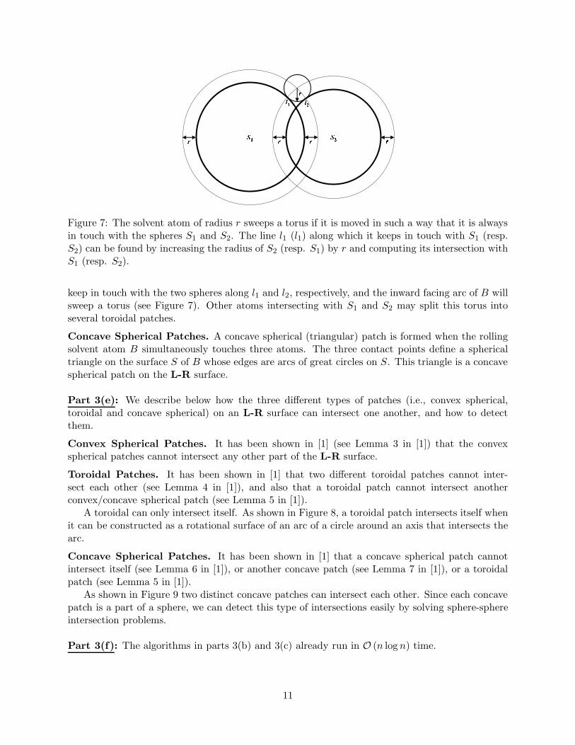
¶ ¶¶·¸ ·¹º¸ º¹¶ ¶Figure 7: The solvent atom of radius r sweeps a torus if it is moved in such a way that it is alwaysin touch with the spheres S1 and S2. The line l1 (l1) along which it keeps in touch with S1 (resp.S2) can be found by increasing the radius of S2 (resp. S1) by r and computing its intersection withS1 (resp. S2).

keep in touch with the two spheres along l1 and l2, respectively, and the inward facing arc of B willsweep a torus (see Figure 7). Other atoms intersecting with S1 and S2 may split this torus intoseveral toroidal patches.

Concave Spherical Patches. A concave spherical (triangular) patch is formed when the rollingsolvent atom B simultaneously touches three atoms. The three contact points define a sphericaltriangle on the surface S of B whose edges are arcs of great circles on S. This triangle is a concavespherical patch on the L-R surface.

Part 3(e): We describe below how the three different types of patches (i.e., convex spherical,toroidal and concave spherical) on an L-R surface can intersect one another, and how to detectthem.

Convex Spherical Patches. It has been shown in [1] (see Lemma 3 in [1]) that the convexspherical patches cannot intersect any other part of the L-R surface.

Toroidal Patches. It has been shown in [1] that two different toroidal patches cannot inter-sect each other (see Lemma 4 in [1]), and also that a toroidal patch cannot intersect anotherconvex/concave spherical patch (see Lemma 5 in [1]).

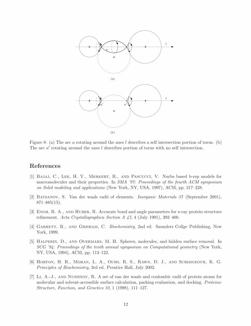
A toroidal can only intersect itself. As shown in Figure 8, a toroidal patch intersects itself whenit can be constructed as a rotational surface of an arc of a circle around an axis that intersects thearc.

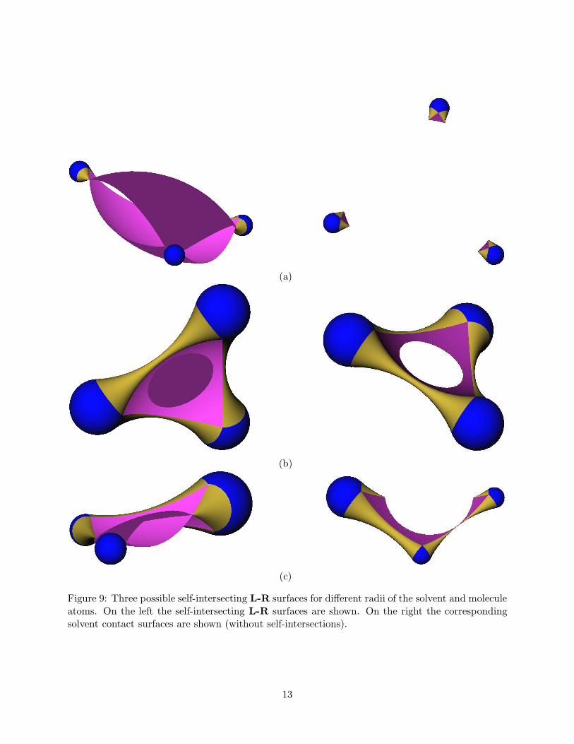
Concave Spherical Patches. It has been shown in [1] that a concave spherical patch cannotintersect itself (see Lemma 6 in [1]), or another concave patch (see Lemma 7 in [1]), or a toroidalpatch (see Lemma 5 in [1]).

As shown in Figure 9 two distinct concave patches can intersect each other. Since each concavepatch is a part of a sphere, we can detect this type of intersections easily by solving sphere-sphereintersection problems.

Part 3(f): The algorithms in parts 3(b) and 3(c) already run in O (n log n) time.

11

a

l

a′

l

(a)

(b)

a′

Figure 8: (a) The arc a rotating around the axes l describes a self intersection portion of torus. (b)The arc a′ rotating around the axes l describes portion of torus with no self intersection.

References

[1] Bajaj, C., Lee, H. Y., Merkert, R., and Pascucci, V. Nurbs based b-rep models formacromolecules and their properties. In SMA ’97: Proceedings of the fourth ACM symposiumon Solid modeling and applications (New York, NY, USA, 1997), ACM, pp. 217–228.

[2] Batsanov, S. Van der waals radii of elements. Inorganic Materials 37 (September 2001),871–885(15).

[3] Engh, R. A., and Huber, R. Accurate bond and angle parameters for x-ray protein structurerefinement. Acta Crystallographica Section A 47, 4 (July 1991), 392–400.

[4] Garrett, R., and Grisham, C. Biochemistry, 2nd ed. Saunders Collge Publishing, NewYork, 1999.

[5] Halperin, D., and Overmars, M. H. Spheres, molecules, and hidden surface removal. InSCG ’94: Proceedings of the tenth annual symposium on Computational geometry (New York,NY, USA, 1994), ACM, pp. 113–122.

[6] Horton, H. R., Moran, L. A., Ochs, R. S., Rawn, D. J., and Scrimgeour, K. G.

Principles of Biochemistry, 3rd ed. Prentice Hall, July 2002.

[7] Li, A.-J., and Nussinov, R. A set of van der waals and coulombic radii of protein atoms formolecular and solvent-accessible surface calculation, packing evaluation, and docking. Proteins:Structure, Function, and Genetics 32, 1 (1998), 111–127.

12

(a)

(b)

(c)

Figure 9: Three possible self-intersecting L-R surfaces for different radii of the solvent and moleculeatoms. On the left the self-intersecting L-R surfaces are shown. On the right the correspondingsolvent contact surfaces are shown (without self-intersections).

13

[8] Schlick, T. Molecular Modeling and Simulation: An Interdisciplinary Guide. Springer-VerlagNew York, Inc., Secaucus, NJ, USA, 2002.

14