Lecture 17: Smoothing splines, Local Regression, and … · Lecture 17: Smoothing splines, Local...
51
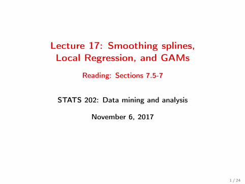
Lecture 17: Smoothing splines, Local Regression, and GAMs Reading: Sections 7.5-7 STATS 202: Data mining and analysis November 6, 2017 1 / 24
-
Upload
vuongtuong -
Category
Documents
-
view
232 -
download
4
Transcript of Lecture 17: Smoothing splines, Local Regression, and … · Lecture 17: Smoothing splines, Local...
Lecture 17: Smoothing splines,Local Regression, and GAMs
Reading: Sections 7.5-7
STATS 202: Data mining and analysis
November 6, 2017
1 / 24
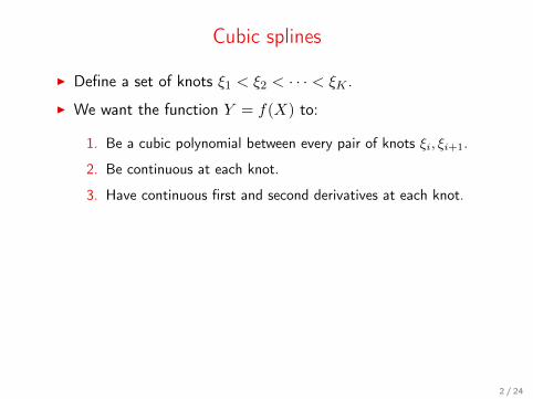
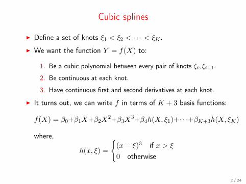
Cubic splines
I Define a set of knots ξ1 < ξ2 < · · · < ξK .
I We want the function Y = f(X) to:
1. Be a cubic polynomial between every pair of knots ξi, ξi+1.
2. Be continuous at each knot.
3. Have continuous first and second derivatives at each knot.
I It turns out, we can write f in terms of K + 3 basis functions:
f(X) = β0+β1X+β2X2+β3X
3+β4h(X, ξ1)+· · ·+βK+3h(X, ξK)
where,
h(x, ξ) =
(x− ξ)3 if x > ξ
0 otherwise
2 / 24
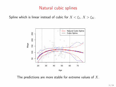
Natural cubic splines
Spline which is linear instead of cubic for X < ξ1, X > ξK .
20 30 40 50 60 70
50
10
01
50
20
02
50
Age
Wa
ge
Natural Cubic Spline
Cubic Spline
The predictions are more stable for extreme values of X.
3 / 24
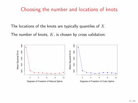
Choosing the number and locations of knots
The locations of the knots are typically quantiles of X.
The number of knots, K, is chosen by cross validation:
2 4 6 8 10
16
00
16
20
16
40
16
60
16
80
Degrees of Freedom of Natural Spline
Me
an
Sq
ua
red
Err
or
2 4 6 8 10
16
00
16
20
16
40
16
60
16
80
Degrees of Freedom of Cubic Spline
Me
an
Sq
ua
red
Err
or
4 / 24

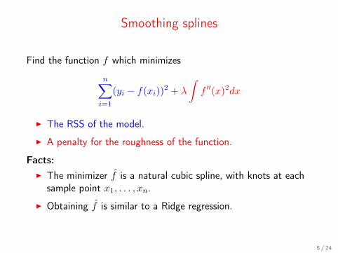
Smoothing splines
Find the function f which minimizes
n∑i=1
(yi − f(xi))2 + λ
∫f ′′(x)2dx
I The RSS of the model.
I A penalty for the roughness of the function.
Facts:I The minimizer f is a natural cubic spline, with knots at each
sample point x1, . . . , xn.
I Obtaining f is similar to a Ridge regression.
5 / 24
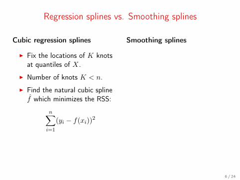
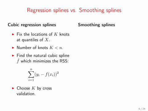
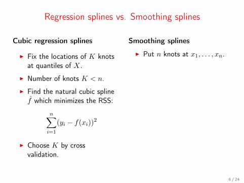
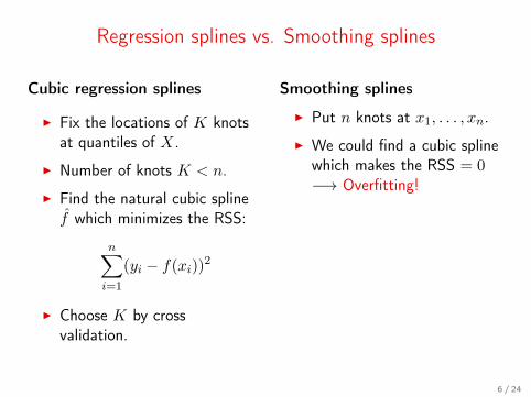
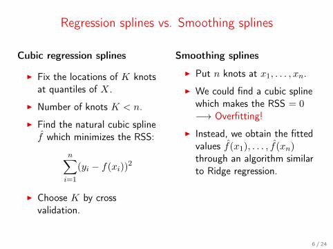
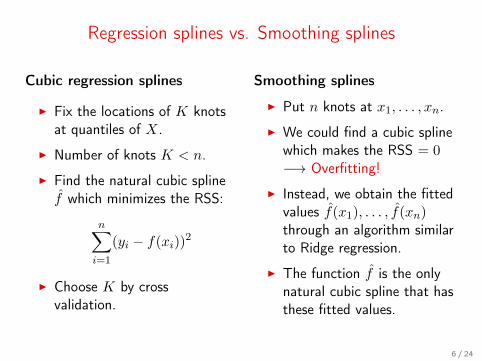
Regression splines vs. Smoothing splines
Cubic regression splines Smoothing splines
I Fix the locations of K knotsat quantiles of X.
I Number of knots K < n.
I Find the natural cubic splinef which minimizes the RSS:
n∑i=1
(yi − f(xi))2
I Choose K by crossvalidation.
I Put n knots at x1, . . . , xn.
I We could find a cubic splinewhich makes the RSS = 0−→ Overfitting!
I Instead, we obtain the fittedvalues f(x1), . . . , f(xn)through an algorithm similarto Ridge regression.
I The function f is the onlynatural cubic spline that hasthese fitted values.
6 / 24
Deriving a smoothing spline
1. Show that if you fix the values f(x1), . . . , f(xn), the roughness∫f ′′(x)2dx
is minimized by a natural cubic spline. Problem 5.7 in ESL.
2. Deduce that the solution to the smoothing spline problem is anatural cubic spline, which can be written in terms of its basisfunctions.
f(x) = β0 + β1f1(x) + . . . βn+3fn+3(x)
7 / 24
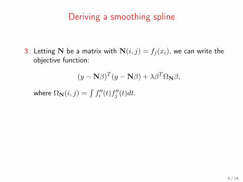
Deriving a smoothing spline
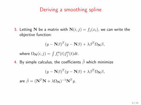
3. Letting N be a matrix with N(i, j) = fj(xi), we can write theobjective function:
(y −Nβ)T (y −Nβ) + λβTΩNβ,
where ΩN(i, j) =∫f ′′i (t)f ′′j (t)dt.
4. By simple calculus, the coefficients β which minimize
(y −Nβ)T (y −Nβ) + λβTΩNβ,
are β = (NTN + λΩN)−1NT y.
8 / 24
Deriving a smoothing spline
3. Letting N be a matrix with N(i, j) = fj(xi), we can write theobjective function:
(y −Nβ)T (y −Nβ) + λβTΩNβ,
where ΩN(i, j) =∫f ′′i (t)f ′′j (t)dt.
4. By simple calculus, the coefficients β which minimize
(y −Nβ)T (y −Nβ) + λβTΩNβ,
are β = (NTN + λΩN)−1NT y.
8 / 24
Deriving a smoothing spline
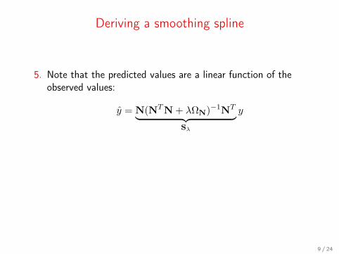
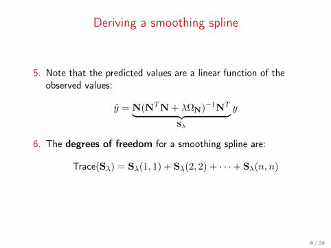
5. Note that the predicted values are a linear function of theobserved values:
y = N(NTN + λΩN)−1NT︸ ︷︷ ︸Sλ
y
6. The degrees of freedom for a smoothing spline are:
Trace(Sλ) = Sλ(1, 1) + Sλ(2, 2) + · · ·+ Sλ(n, n)
9 / 24
Deriving a smoothing spline
5. Note that the predicted values are a linear function of theobserved values:
y = N(NTN + λΩN)−1NT︸ ︷︷ ︸Sλ
y
6. The degrees of freedom for a smoothing spline are:
Trace(Sλ) = Sλ(1, 1) + Sλ(2, 2) + · · ·+ Sλ(n, n)
9 / 24
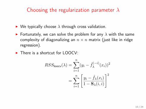
Choosing the regularization parameter λ
I We typically choose λ through cross validation.
I Fortunately, we can solve the problem for any λ with the samecomplexity of diagonalizing an n× n matrix (just like in ridgeregression).
I There is a shortcut for LOOCV:
RSSloocv(λ) =n∑i=1
(yi − f (−i)λ (xi))2
=
n∑i=1
[yi − fλ(xi)
1− Sλ(i, i)
]2
10 / 24

Choosing the regularization parameter λ
I We typically choose λ through cross validation.
I Fortunately, we can solve the problem for any λ with the samecomplexity of diagonalizing an n× n matrix (just like in ridgeregression).
I There is a shortcut for LOOCV:
RSSloocv(λ) =
n∑i=1
(yi − f (−i)λ (xi))2
=
n∑i=1
[yi − fλ(xi)
1− Sλ(i, i)
]2
10 / 24
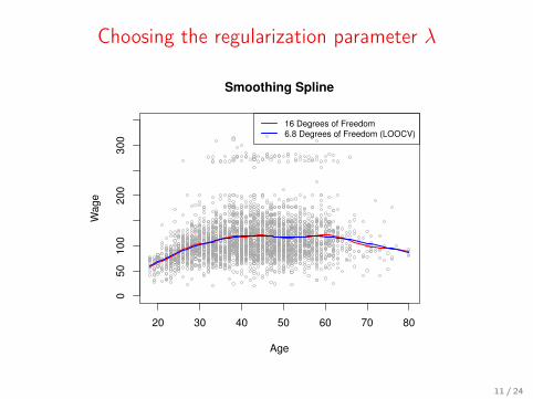
Choosing the regularization parameter λ
20 30 40 50 60 70 80
050
100
200
300
Age
Wage
Smoothing Spline
16 Degrees of Freedom
6.8 Degrees of Freedom (LOOCV)
11 / 24

Regression splines vs. Smoothing splines
Cubic regression splines Smoothing splines
I Fix the locations of K knotsat quantiles of X.
I Number of knots K < n.
I Find the natural cubic splinef which minimizes the RSS:
n∑i=1
(yi − f(xi))2
I Choose K by crossvalidation.
I Put n knots at x1, . . . , xn.
I We could find a cubic splinewhich makes the RSS = 0−→ Overfitting!
I Instead, we obtain the fittedvalues f(x1), . . . , f(xn)through an algorithm similarto Ridge regression.
I The function f is the onlynatural cubic spline that hasthese fitted values.
12 / 24
Local linear regression
0.0 0.2 0.4 0.6 0.8 1.0
−1
.0−
0.5
0.0
0.5
1.0
1.5
O
O
O
O
O
OO
O
O
O
O
O
O
O
O
OOO
O
O
O
O
O
O
O
O
OO
O
O
OO
O
O
O
O
O
O
OO
O
O
O
O
O
O
O
O
O
O
OO
O
O
O
O
O
OO
O
O
O
O
OO
O
O
OO
O
O
O
OO
O
O
O
O
O
O
O
OO
O
O
O
OO
O
O
O
O
OO
O
O
O
O
O
O
O
O
O
O
O
OO
O
O
O
O
O
O
O
O
OOO
O
O
O
O
0.0 0.2 0.4 0.6 0.8 1.0
−1
.0−
0.5
0.0
0.5
1.0
1.5
O
O
O
O
O
OO
O
O
O
O
O
O
O
O
OOO
O
O
O
O
O
O
O
O
OO
O
O
OO
O
O
O
O
O
O
OO
O
O
O
O
O
O
O
O
O
O
OO
O
O
O
O
O
OO
O
O
O
O
OO
O
O
OO
O
O
O
OO
O
O
O
O
O
O
O
OO
O
O
O
OO
O
O
O
O
OO
O
O
O
O
O
O
O
O
O
O
O
OO
O
O
OO
O
O
O
O
O
O
OO
O
O
O
O
O
O
O
O
O
O
OO
O
O
O
O
O
OO
O
O
O
O
OO
O
O
OO
O
O
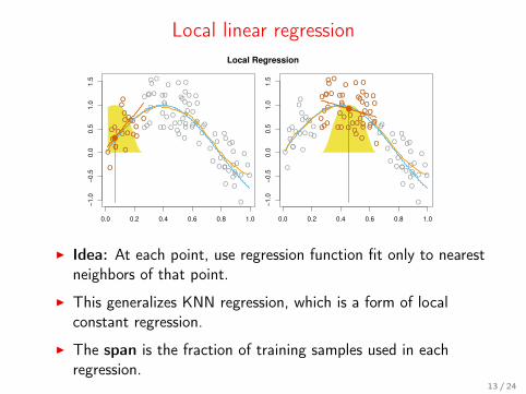
Local Regression
I Idea: At each point, use regression function fit only to nearestneighbors of that point.
I This generalizes KNN regression, which is a form of localconstant regression.
I The span is the fraction of training samples used in eachregression.
13 / 24
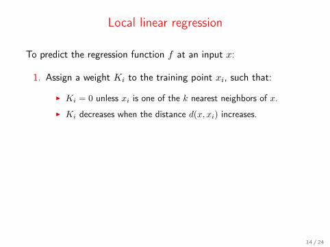
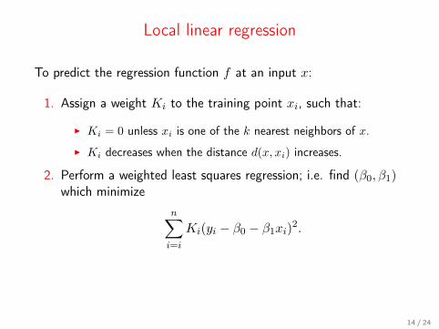
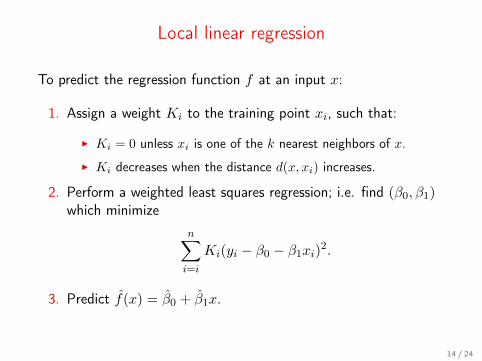
Local linear regression
To predict the regression function f at an input x:
1. Assign a weight Ki to the training point xi, such that:
I Ki = 0 unless xi is one of the k nearest neighbors of x.
I Ki decreases when the distance d(x, xi) increases.
2. Perform a weighted least squares regression; i.e. find (β0, β1)which minimize
n∑i=i
Ki(yi − β0 − β1xi)2.
3. Predict f(x) = β0 + β1x.
14 / 24
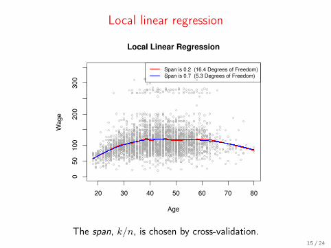
Local linear regression
20 30 40 50 60 70 80
050
100
200
300
Age
Wage
Local Linear Regression
Span is 0.2 (16.4 Degrees of Freedom)
Span is 0.7 (5.3 Degrees of Freedom)
The span, k/n, is chosen by cross-validation.15 / 24
Generalized Additive Models (GAMs)
Extension of non-linear models to multiple predictors:
wage = β0 + β1 × year + β2 × age + β3 × education + ε
−→ wage = β0 + f1(year) + f2(age) + f3(education) + ε
The functions f1, . . . , fp can be polynomials, natural splines,smoothing splines, local regressions...
16 / 24
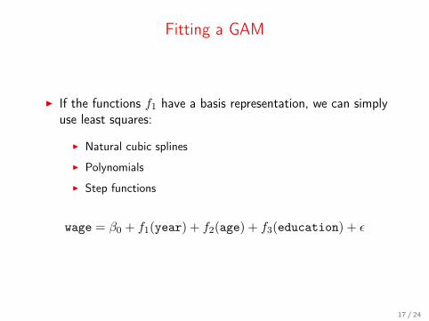
Fitting a GAM
I If the functions f1 have a basis representation, we can simplyuse least squares:
I Natural cubic splines
I Polynomials
I Step functions
wage = β0 + f1(year) + f2(age) + f3(education) + ε
17 / 24
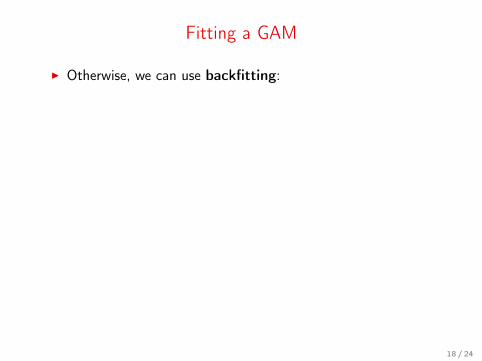
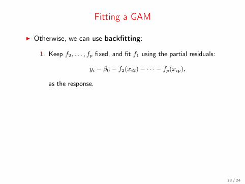
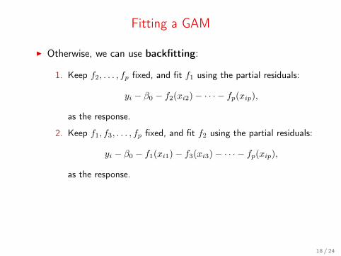
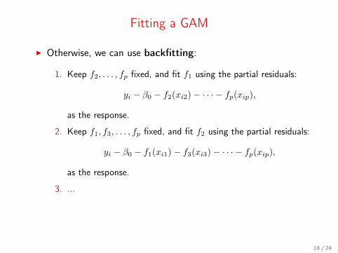
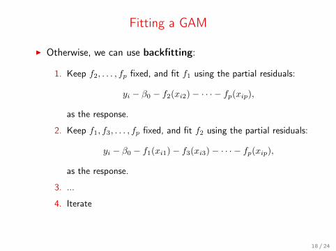
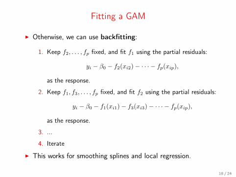
Fitting a GAM
I Otherwise, we can use backfitting:
1. Keep f2, . . . , fp fixed, and fit f1 using the partial residuals:
yi − β0 − f2(xi2)− · · · − fp(xip),
as the response.
2. Keep f1, f3, . . . , fp fixed, and fit f2 using the partial residuals:
yi − β0 − f1(xi1)− f3(xi3)− · · · − fp(xip),
as the response.
3. ...
4. Iterate
I This works for smoothing splines and local regression.
18 / 24
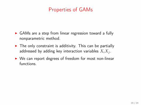
Properties of GAMs
I GAMs are a step from linear regression toward a fullynonparametric method.
I The only constraint is additivity. This can be partiallyaddressed by adding key interaction variables XiXj .
I We can report degrees of freedom for most non-linearfunctions.
I As in linear regression, we can examine the significance of eachof the variables.
19 / 24

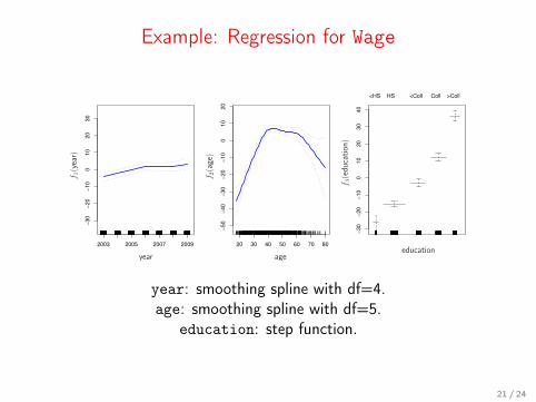
Example: Regression for Wage
2003 2005 2007 2009
−30
−20
−10
010
20
30
20 30 40 50 60 70 80
−50
−40
−30
−20
−10
010
20
−30
−20
−10
010
20
30
40
<HS HS <Coll Coll >Coll
f 1(year)
f 2(age)
f 3(edu
cation)
year ageeducation
year: natural spline with df=4.age: natural spline with df=5.education: step function.
20 / 24
Example: Regression for Wage
2003 2005 2007 2009
−30
−20
−10
010
20
30
20 30 40 50 60 70 80
−50
−40
−30
−20
−10
010
20
−30
−20
−10
010
20
30
40
<HS HS <Coll Coll >Coll
f 1(year)
f 2(age)
f 3(edu
cation)
year ageeducation
year: smoothing spline with df=4.age: smoothing spline with df=5.
education: step function.
21 / 24
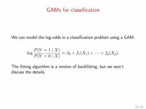
GAMs for classification
We can model the log-odds in a classification problem using a GAM:
logP (Y = 1 | X)
P (Y = 0 | X)= β0 + f1(X1) + · · ·+ fp(Xp).
The fitting algorithm is a version of backfitting, but we won’tdiscuss the details.
22 / 24
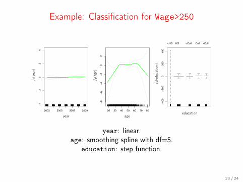
Example: Classification for Wage>250
2003 2005 2007 2009
−4
−2
02
4
20 30 40 50 60 70 80
−8
−6
−4
−2
02
−400
−200
0200
400
<HS HS <Coll Coll >Coll
f 1(year)
f 2(age)
f 3(edu
cation)
year ageeducation
year: linear.age: smoothing spline with df=5.
education: step function.
23 / 24
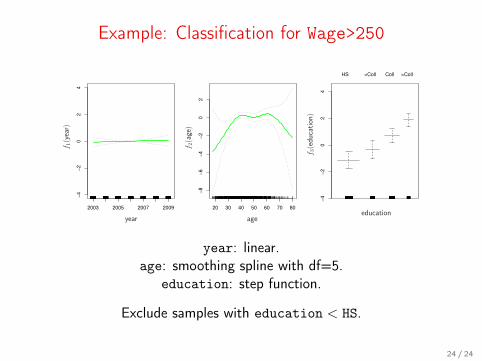
Example: Classification for Wage>250
2003 2005 2007 2009
−4
−2
02
4
20 30 40 50 60 70 80
−8
−6
−4
−2
02
−4
−2
02
4
HS <Coll Coll >Coll
f 1(year)
f 2(age)
f 3(edu
cation)
year ageeducation
year: linear.age: smoothing spline with df=5.
education: step function.
Exclude samples with education < HS.
24 / 24