18.369 Problem Set 4 Solutions - Math.mit.edumath.mit.edu/~stevenj/18.369/pset4sol-spring18.pdf ·...
10
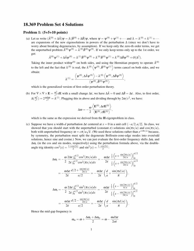
18.369 Problem Set 4 Solutions Problem 1: (5+5+10 points) (a) Let us write ( ˆ A (0) + Δ ˆ A)ψ = λ ( ˆ B (0) + Δ ˆ B)ψ , where ψ = ψ (0) + ψ (1) + ··· and λ = λ (0) + λ (1) + ··· are expansions of the new eigensolutions in powers of the perturbation Δ (since we don’t have to worry about breaking degeneracies, by assumption). If we keep only the zero-th order terms, we get the unperturbed problem ˆ A (0) ψ (0) = λ (0) ˆ B (0) ψ (0) . If we only keep terms only up to the 1st order, we get: ˆ A (0) ψ (1) + Δ ˆ Aψ (0) = λ (1) ˆ B (0) ψ (0) + λ (0) ˆ B (0) ψ (1) + λ (0) Δ ˆ Bψ (0) + O(Δ 2 ). Taking the inner product withψ (0) on both sides, and using the Hermitian property to operate ˆ A (0) to the left and the fact that λ (0) is real, the λ (0) D ψ (0) , ˆ B (0) ψ (1) E terms cancel on both sides, and we obtain: λ (1) = D ψ (0) , Δ ˆ Aψ (0) E - λ (0) D ψ (0) , Δ ˆ Bψ (0) E ψ (0) , ˆ B (0) ψ (0) , which is the generalized version of first-order perturbation theory. (b) For ∇ × ∇ × E = ω 2 c 2 ε E with a small change Δε , we have Δ ˆ A = 0 and Δ ˆ B = Δε . Also, to first order, Δ( ω 2 c 2 )= 2 ωΔω c 2 = λ (1) . Plugging this in above and dividing through by 2ω /c 2 , we have: Δω = - ω 2 D E (0) , Δε E (0) E E (0) , ε E (0) , which is the same as the expression we derived from the H eigenproblem in class. (c) Suppose we have a width-d perturbation Δε centered at x = 0 in a unit cell (-a/2, a/2]. In class, we showed that you should start with the unperturbed (constant ε ) solutions sin(π x/a) and cos(π x/a), both with unperturbed frequency ω = cπ /a √ ε . (We used these solutions rather than e ±iπ x/a because, by symmetry, the perturbation must split the degenerate Brillouin-zone-edge modes into even/odd solutions, hence sine and cosine.) Now, we can just evaluate the first-order frequency shifts Δω c and Δω s (in the cos and sin modes, respectively) using the perturbation formula above, via the double- angle trig identity cos 2 (x)= 1+cos(2x) 2 and sin 2 (x)= 1-cos(2x) 2 : Δω c = - ω 2 2Δε R d/2 0 cos 2 (π x/a)dx 2ε R a/2 0 cos 2 (π x/a)dx = - ω Δε 2ε 1 2 x + sin(2π x/a) 2π /a d/2 0 1 2 x + sin(2π x/a) 2π /a a/2 0 = - ω Δε 2ε d /2 + sin(π d/a) 2π /a a/2 = - ω Δε 2ε d a + sin(π d /a) π . Δω s = - ω 2 2Δε R d/2 0 sin 2 (π x/a)dx 2ε R a/2 0 sin 2 (π x/a)dx = - ω Δε 2ε 1 2 x - sin(2π x/a) π /a d/2 0 1 2 x - sin(2π x/a) 2π /a a/2 0 = - ω Δε 2ε d /2 - sin(π d/a) 2π /a a/2 = - ω Δε 2ε d a - sin(π d /a) π . Hence the mid-gap frequency is ω m = ω + Δω c + Δω m 2 = ω - ω d Δε 2aε 1
Transcript of 18.369 Problem Set 4 Solutions - Math.mit.edumath.mit.edu/~stevenj/18.369/pset4sol-spring18.pdf ·...
18.369 Problem Set 4 Solutions
Problem 1: (5+5+10 points)(a) Let us write (A(0)+∆A)ψ = λ (B(0)+∆B)ψ , where ψ = ψ(0)+ψ(1)+ · · · and λ = λ (0)+λ (1)+ · · ·
are expansions of the new eigensolutions in powers of the perturbation ∆ (since we don’t have toworry about breaking degeneracies, by assumption). If we keep only the zero-th order terms, we getthe unperturbed problem A(0)ψ(0) = λ (0)B(0)ψ(0). If we only keep terms only up to the 1st order, weget:
A(0)ψ
(1)+∆Aψ(0) = λ
(1)B(0)ψ
(0)+λ(0)B(0)
ψ(1)+λ
(0)∆Bψ
(0)+O(∆2).
Taking the inner product withψ(0) on both sides, and using the Hermitian property to operate A(0)
to the left and the fact that λ (0) is real, the λ (0)⟨
ψ(0), B(0)ψ(1)⟩
terms cancel on both sides, and weobtain:
λ(1) =
⟨ψ(0),∆Aψ(0)
⟩−λ (0)
⟨ψ(0),∆Bψ(0)
⟩⟨ψ(0), B(0)ψ(0)
⟩ ,
which is the generalized version of first-order perturbation theory.
(b) For ∇×∇×E = ω2
c2 εE with a small change ∆ε , we have ∆A = 0 and ∆B = ∆ε . Also, to first order,
∆(ω2
c2 ) = 2 ω∆ω
c2 = λ (1). Plugging this in above and dividing through by 2ω/c2, we have:
∆ω =−ω
2
⟨E(0),∆εE(0)
⟩⟨E(0),εE(0)
⟩ ,
which is the same as the expression we derived from the H eigenproblem in class.
(c) Suppose we have a width-d perturbation ∆ε centered at x = 0 in a unit cell (−a/2,a/2]. In class, weshowed that you should start with the unperturbed (constant ε) solutions sin(πx/a) and cos(πx/a),both with unperturbed frequency ω = cπ/a
√ε . (We used these solutions rather than e±iπx/a because,
by symmetry, the perturbation must split the degenerate Brillouin-zone-edge modes into even/oddsolutions, hence sine and cosine.) Now, we can just evaluate the first-order frequency shifts ∆ωc and∆ωs (in the cos and sin modes, respectively) using the perturbation formula above, via the double-angle trig identity cos2(x) = 1+cos(2x)
2 and sin2(x) = 1−cos(2x)2 :
∆ωc =−ω
22∆ε
∫ d/20 cos2(πx/a)dx
2ε∫ a/2
0 cos2(πx/a)dx=−ω∆ε
2ε
12
(x+ sin(2πx/a)
2π/a
)∣∣∣d/2
0
12
(x+ sin(2πx/a)
2π/a
)∣∣∣a/2
0
=−ω∆ε
2ε
d/2+ sin(πd/a)2π/a
a/2=−ω∆ε
2ε
(da+
sin(πd/a)π
).
∆ωs =−ω
22∆ε
∫ d/20 sin2(πx/a)dx
2ε∫ a/2
0 sin2(πx/a)dx=−ω∆ε
2ε
12
(x− sin(2πx/a)
π/a
)∣∣∣d/2
0
12
(x− sin(2πx/a)
2π/a
)∣∣∣a/2
0
=−ω∆ε
2ε
d/2− sin(πd/a)2π/a
a/2=−ω∆ε
2ε
(da− sin(πd/a)
π
).
Hence the mid-gap frequency is
ωm = ω +∆ωc +∆ωm
2= ω− ωd∆ε
2aε
1
and the gap width is
∆ω = ∆ωs−∆ωc =ω∆ε
ε
sin(πd/a)π
,
so we obtain:∆ω
ωm=
∆ε
ε
sin(πd/a)π
+O(∆ε2)
as desired (note that the ∆ε term in ωm contributes only to second order in ∆ω/ωm).
Problem 2: (20 points)
What Calvin has forgotten is that, with Bloch’s theorem, the periodicity in k is determined by the choice ofunit cell—if you employ a supercell, a periodicity larger than the minimum, then this leads to a labelling kthat is “folded” onto the smaller Brillouin zone of the new unit cell.
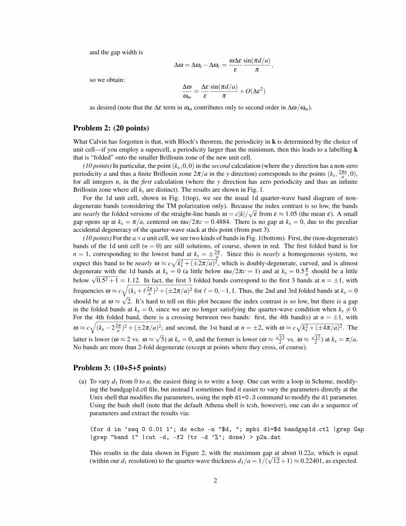
(10 points) In particular, the point (kx,0,0) in the second calculation (where the y direction has a non-zeroperiodicity a and thus a finite Brillouin zone 2π/a in the y direction) corresponds to the points (kx,
2πna ,0),
for all integers n, in the first calculation (where the y direction has zero periodicity and thus an infiniteBrillouin zone where all ky are distinct). The results are shown in Fig. 1.
For the 1d unit cell, shown in Fig. 1(top), we see the usual 1d quarter-wave band diagram of non-degenerate bands (considering the TM polarization only). Because the index contrast is so low, the bandsare nearly the folded versions of the straight-line bands ω = c|k|/
√ε from ε ≈ 1.05 (the mean ε). A small
gap opens up at kx = π/a, centered on ωa/2πc = 0.4884. There is no gap at kx = 0, due to the peculiaraccidental degeneracy of the quarter-wave stack at this point (from pset 3).
(10 points) For the a×a unit cell, we see two kinds of bands in Fig. 1(bottom). First, the (non-degenerate)bands of the 1d unit cell (n = 0) are still solutions, of course, shown in red. The first folded band is forn = 1, corresponding to the lowest band at ky = ± 2π
a . Since this is nearly a homogeneous system, weexpect this band to be nearly ω ≈ c
√k2
x +(±2π/a)2, which is doubly-degenerate, curved, and is almostdegenerate with the 1d bands at kx = 0 (a little below ωa/2πc = 1) and at kx = 0.5 π
a should be a littlebelow
√0.52 +1 = 1.12. In fact, the first 3 folded bands correspond to the first 3 bands at n = ±1, with
frequencies ω ≈ c√(kx + ` 2π
a )2 +(±2π/a)2 for `= 0,−1,1. Thus, the 2nd and 3rd folded bands at kx = 0
should be at ω ≈√
2. It’s hard to tell on this plot because the index contrast is so low, but there is a gapin the folded bands at kx = 0, since we are no longer satisfying the quarter-wave condition when ky 6= 0.For the 4th folded band, there is a crossing between two bands: first, the 4th band(s) at n = ±1, with
ω ≈ c√(kx−2 2π
a )2 +(±2π/a)2; and second, the 1st band at n = ±2, with ω ≈ c√
k2x +(±4π/a)2. The
latter is lower (ω ≈ 2 vs. ω ≈√
5) at kx = 0, and the former is lower (ω ≈√
132 vs. ω ≈
√172 ) at kx = π/a.
No bands are more than 2-fold degenerate (except at points where they cross, of course).
Problem 3: (10+5+5 points)
(a) To vary d1 from 0 to a, the easiest thing is to write a loop. One can write a loop in Scheme, modify-ing the bandgap1d.ctl file, but instead I sometimes find it easier to vary the parameters directly at theUnix shell that modifies the parameters, using the mpb d1=0.3 command to modify the d1 parameter.Using the bash shell (note that the default Athena shell is tcsh, however), one can do a sequence ofparameters and extract the results via:
(for d in ‘seq 0 0.01 1‘; do echo -n "$d, "; mpbi d1=$d bandgap1d.ctl |grep Gap|grep "band 1" |cut -d, -f2 |tr -d ’%’; done) > p2a.dat
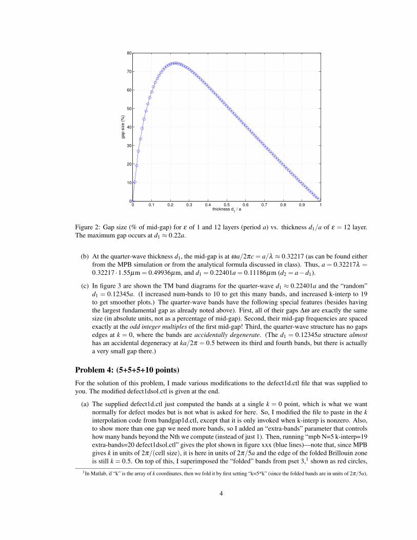
This results in the data shown in Figure 2, with the maximum gap at about 0.22a, which is equal(within our d1 resolution) to the quarter-wave thickness d1/a = 1/(
√12+1)≈ 0.22401, as expected.
2
0 0.1 0.2 0.3 0.4 0.50
0.5
1
1.5
2fr
equency (
2πc/a
)
kx (2π/a)
0 0.1 0.2 0.3 0.4 0.50
0.5
1
1.5
2
frequency (
2πc/a
)
kx (2π/a)
1d cell
1d cell
folded 2x degenerate
Figure 1: Band diagrams of quarter-wave stack (ε = 1.1/1). Top: 1d unit cell. Bottom: 2d unit cell (super-cell), showing 1d bands (red) and double-degenerate folded bands from ky =
2πna for n 6= 0 (blue).
3
0 0.1 0.2 0.3 0.4 0.5 0.6 0.7 0.8 0.9 10
10
20
30
40
50
60
70
80
thickness d1 / a
gap s
ize (
%)
Figure 2: Gap size (% of mid-gap) for ε of 1 and 12 layers (period a) vs. thickness d1/a of ε = 12 layer.The maximum gap occurs at d1 ≈ 0.22a.
(b) At the quarter-wave thickness d1, the mid-gap is at ωa/2πc = a/λ ≈ 0.32217 (as can be found eitherfrom the MPB simulation or from the analytical formula discussed in class). Thus, a = 0.32217λ =0.32217 ·1.55µm = 0.49936µm, and d1 = 0.22401a = 0.11186µm (d2 = a−d1).
(c) In figure 3 are shown the TM band diagrams for the quarter-wave d1 ≈ 0.22401a and the “random”d1 = 0.12345a. (I increased num-bands to 10 to get this many bands, and increased k-interp to 19to get smoother plots.) The quarter-wave bands have the following special features (besides havingthe largest fundamental gap as already noted above). First, all of their gaps ∆ω are exactly the samesize (in absolute units, not as a percentage of mid-gap). Second, their mid-gap frequencies are spacedexactly at the odd integer multiples of the first mid-gap! Third, the quarter-wave structure has no gapsedges at k = 0, where the bands are accidentally degenerate. (The d1 = 0.12345a structure almosthas an accidental degeneracy at ka/2π = 0.5 between its third and fourth bands, but there is actuallya very small gap there.)
Problem 4: (5+5+5+10 points)For the solution of this problem, I made various modifications to the defect1d.ctl file that was supplied toyou. The modified defect1dsol.ctl is given at the end.
(a) The supplied defect1d.ctl just computed the bands at a single k = 0 point, which is what we wantnormally for defect modes but is not what is asked for here. So, I modified the file to paste in the kinterpolation code from bandgap1d.ctl, except that it is only invoked when k-interp is nonzero. Also,to show more than one gap we need more bands, so I added an “extra-bands” parameter that controlshow many bands beyond the Nth we compute (instead of just 1). Then, running “mpb N=5 k-interp=19extra-bands=20 defect1dsol.ctl” gives the plot shown in figure xxx (blue lines)—note that, since MPBgives k in units of 2π/(cell size), it is here in units of 2π/5a and the edge of the folded Brillouin zoneis still k = 0.5. On top of this, I superimposed the “folded” bands from pset 3,1 shown as red circles,
1In Matlab, if “k” is the array of k coordinates, then we fold it by first setting “k=5*k” (since the folded bands are in units of 2π/5a),
4

0 0.05 0.1 0.15 0.2 0.25 0.3 0.35 0.4 0.45 0.50
0.5
1
1.5
2
2.5
3
k (2π/a)
ω (
2πc/a
)
quarter−wave
d1 = 0.12345a
Figure 3: TM band diagram of ε = 12/1 multilayer film, with quarter-wave thickness d1 ≈ 0.22401a (blue,solid) or thickness d1 = 0.12345a (red, dashed) of the ε = 12 layer. Quarter-wave gaps are shaded blue.
and we can see that they exactly coincide as expected.
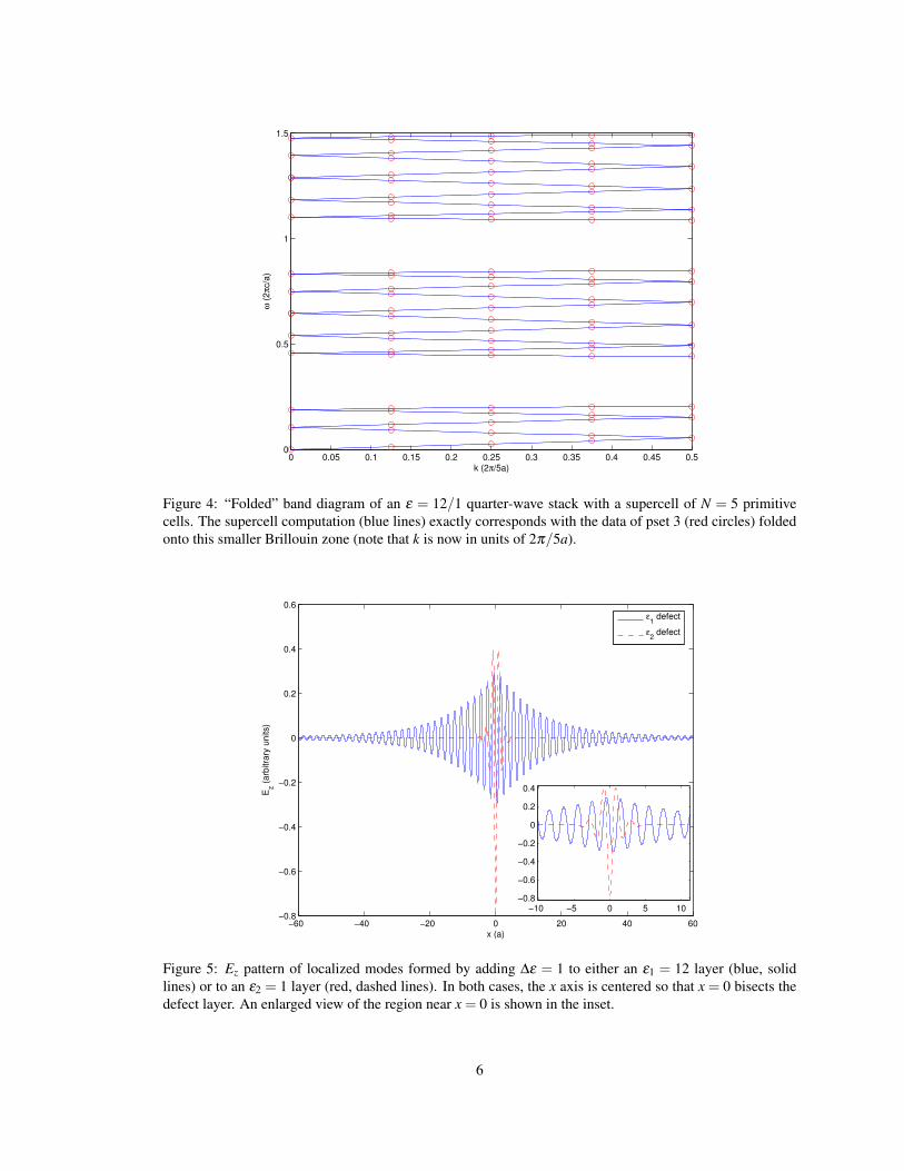
(b) When we increase the ε of a layer, it pulls down a band from the upper edge of the gap, and thus welook at band N +1 in the supercell to get the defect mode. The supplied input file is set up to increasethe ε of an ε2 layer by the parameter “deps2”. To change an ε1 layer, the easiest thing is just to swap ε1and ε2: “mpb eps1=1 eps2=12 deps2=1 defect1d.ctl”. Unfortunately, it turns out that the ε1 defect israther weakly confined, so we also set our supercell size to N = 120 (I increased it until I saw clearlylocalized modes). The resulting Ez field patterns, increasing ε1 or ε2 by ∆ε = 1, are shown in figure 5.
From the inset of figure 5, we can see that the ε1 defect mode is odd and the ε2 defect mode iseven through the center of the defect. The reason for this is that both bands are formed by pullingdown the upper band-edge mode at k = π/a (by analytic continuation), and this band edge mode wasodd in the ε1 (high-ε) layer and even in the ε2 (low-ε) layer (as we proved when we found the originof the band gap). From this, we can also see why the ε2 mode is so much more strongly localizedthan the ε1 mode: the latter is odd in the defect layer, and therefore has less field intensity there, andtherefore “feels” the perturbation less strongly, and is therefore less localized.
(c) To make this part a little easier, I modified the .ctl file to only output fields when they are inside thegap (as computed from the unit cell) and to also output the frequencies just in that case. Then I did alittle loop of deps2 values from the bash shell:
(for dep in ‘seq 0 0.1 12‘; do mpbi N=30 deps2=$dep extra-bands=2 defect1dsol.ctl |grep gapfreq;done) > p4c.dat
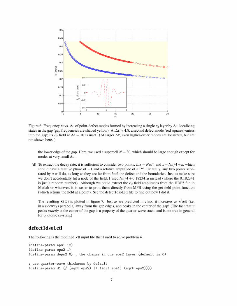
The resulting figure 6 shows the ω as a function of ∆ε of the first two defect modes, where thesecond defect mode (whose Ez is inset for ∆ε = 10) appears in the gap at ∆ε ≈ 4.8. As it turned out,I need to go to larger values of ∆ε , all the way to ∆ε = 30, in order for the first defect mode to reach
and then repeatedly set “k(k > 0.5) = abs(k(k > 0.5) - 1)”.
5
0 0.05 0.1 0.15 0.2 0.25 0.3 0.35 0.4 0.45 0.50
0.5
1
1.5
k (2π/5a)
ω (
2πc/a
)
Figure 4: “Folded” band diagram of an ε = 12/1 quarter-wave stack with a supercell of N = 5 primitivecells. The supercell computation (blue lines) exactly corresponds with the data of pset 3 (red circles) foldedonto this smaller Brillouin zone (note that k is now in units of 2π/5a).
−60 −40 −20 0 20 40 60−0.8
−0.6
−0.4
−0.2
0
0.2
0.4
0.6
x (a)
Ez (
arb
itra
ry u
nits)
−10 −5 0 5 10−0.8
−0.6
−0.4
−0.2
0
0.2
0.4
ε1 defect
ε2 defect
Figure 5: Ez pattern of localized modes formed by adding ∆ε = 1 to either an ε1 = 12 layer (blue, solidlines) or to an ε2 = 1 layer (red, dashed lines). In both cases, the x axis is centered so that x = 0 bisects thedefect layer. An enlarged view of the region near x = 0 is shown in the inset.
6
0 5 10 15 20 25 300
0.05
0.1
0.15
0.2
0.25
0.3
0.35
0.4
0.45
0.5
∆ε
ω (
2πc/a
)
−5 0 5−0.4
−0.2
0
0.2
0.4E
z o
f 2
nd
ba
nd
Figure 6: Frequency ω vs. ∆ε of point-defect modes formed by increasing a single ε2 layer by ∆ε , localizingstates in the gap (gap frequencies are shaded yellow). At ∆ε ≈ 4.8, a second defect mode (red squares) entersinto the gap; its Ez field at ∆ε = 10 is inset. (At larger ∆ε , even higher-order modes are localized, but arenot shown here. )
the lower edge of the gap. Here, we used a supercell N = 30, which should be large enough except formodes at very small ∆ε .
(d) To extract the decay rate, it is sufficient to consider two points, at x = Na/4 and x = Na/4+a, whichshould have a relative phase of −1 and a relative amplitude of e−κa. Or really, any two points sepa-rated by a will do, as long as they are far from both the defect and the boundaries. Just to make surewe don’t accidentally hit a node of the field, I used Na/4+ 0.182341a instead (where the 0.182341is just a random number). Although we could extract the Ez field amplitudes from the HDF5 file inMatlab or whatever, it is easier to print them directly from MPB using the get-field-point function(which returns the field at a point). See the defect1dsol.ctl file to find out how I did it.
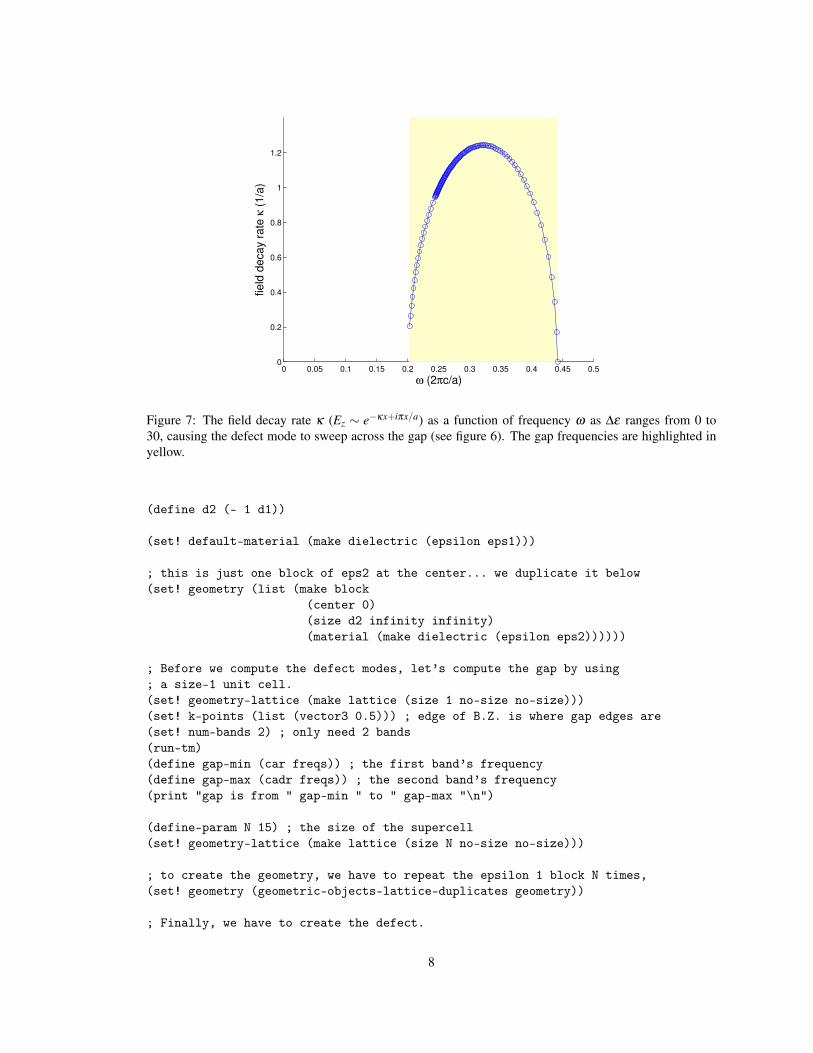
The resulting κ(ω) is plotted in figure 7. Just as we predicted in class, it increases as√
∆ω (i.e.in a sideways parabola) away from the gap edges, and peaks in the center of the gap! (The fact that itpeaks exactly at the center of the gap is a property of the quarter-wave stack, and is not true in generalfor photonic crystals.)
defect1dsol.ctlThe following is the modified .ctl input file that I used to solve problem 4.
(define-param eps1 12)(define-param eps2 1)(define-param deps2 0) ; the change in one eps2 layer (default is 0)
; use quarter-wave thickness by default(define-param d1 (/ (sqrt eps2) (+ (sqrt eps1) (sqrt eps2))))
7
0 0.05 0.1 0.15 0.2 0.25 0.3 0.35 0.4 0.45 0.50
0.2
0.4
0.6
0.8
1
1.2
ω (2πc/a)
fie
ld d
eca
y r
ate
κ (
1/a
)
Figure 7: The field decay rate κ (Ez ∼ e−κx+iπx/a) as a function of frequency ω as ∆ε ranges from 0 to30, causing the defect mode to sweep across the gap (see figure 6). The gap frequencies are highlighted inyellow.
(define d2 (- 1 d1))
(set! default-material (make dielectric (epsilon eps1)))
; this is just one block of eps2 at the center... we duplicate it below(set! geometry (list (make block
(center 0)(size d2 infinity infinity)(material (make dielectric (epsilon eps2))))))
; Before we compute the defect modes, let’s compute the gap by using; a size-1 unit cell.(set! geometry-lattice (make lattice (size 1 no-size no-size)))(set! k-points (list (vector3 0.5))) ; edge of B.Z. is where gap edges are(set! num-bands 2) ; only need 2 bands(run-tm)(define gap-min (car freqs)) ; the first band’s frequency(define gap-max (cadr freqs)) ; the second band’s frequency(print "gap is from " gap-min " to " gap-max "\n")
(define-param N 15) ; the size of the supercell(set! geometry-lattice (make lattice (size N no-size no-size)))
; to create the geometry, we have to repeat the epsilon 1 block N times,(set! geometry (geometric-objects-lattice-duplicates geometry))
; Finally, we have to create the defect.
8
(set! geometry (appendgeometry(list (make block
(center 0)(size d2 infinity infinity)(material (make dielectric
(epsilon (+ eps2 deps2))))))))
(set-param! resolution 32) ; 32 pixels/a
; for the defect mode, k does matter (if the supercell is big enough),; so we just set it to zero. If k-interp is not zero, however, we will; indeed compute the (folded) band structure as in problem 4(a).(define-param k-interp 0)(if (zero? k-interp)
(set! k-points (list (vector3 0)))(set! k-points (interpolate k-interp (list (vector3 0) (vector3 0.5)))))
; because of the folding, the first band (before the gap) will be folded; N times. So, we need to compute N bands plus some extra bands to; get whatever defect states lie in the gap. The number of extra bands; is set by the parameter extra-bands.(define-param extra-bands 1)(set! num-bands (+ N extra-bands))
; Now, instead of outputting all of the modes, we’ll define a little band; function to just output the modes in the gap. A band function is; a function of band index, b; when passed to run, this function is; called for every band computed. We’ll also print the corresponding; frequency so that we can easily grep for it. (See also the MPB manual).(define (output-in-gap b)
(let ((f (list-ref freqs (- b 1)))) ; the frequency of band b(if (and (> f gap-min) (< f gap-max))
(begin(print "gapfreq" b ":, " deps2 ", " f "\n")(output-efield-z b)))))
(run-tm output-in-gap) ; run, outputting Ez
; Now that we’re done, let’s compute the fraction of the field energy; in the defect layer for the last band, for use in getting the slope; domega/d(deps2) for problem 4(d).(get-dfield num-bands) ; get the last band’s D(compute-field-energy) ; compute its epsilon |E|^2 energy density; compute the fraction of the energy in the defect object (center block).(define energy-in-defect (compute-energy-in-objects
(make block(center 0) (size d2 infinity infinity)(material air))))
(print "predicted slope:, " deps2 ", "(* -0.5
(list-ref freqs (- num-bands 1)) ; omega of last band
9
(/ (+ eps2 deps2))energy-in-defect) "\n")
; Finally, for problem 4(f), let’s compute the decay rate by taking the; relative amplitude of the field at a random point and the random point; + a. (Note that the phase should be -1, or a phase angle of 180 degrees).(get-efield num-bands)(define-param fx (+ (/ N 4) 0.182341)) ; a "random" pt. far from the defect(define field-ratio (/ (vector3-z (get-field-point (vector3 fx)))
(vector3-z (get-field-point (vector3 (- fx 1))))))(print "decay:, "
deps2 ", "(list-ref freqs (- num-bands 1)) ", " ; omega of last band(- (log (magnitude field-ratio))) ", " ; decay coefficient kappa(magnitude field-ratio) ", "(rad->deg (angle field-ratio))"\n")
10


![SURP Final Paper [Final] DW](https://static.fdocument.org/doc/165x107/5881c6c61a28ab87638b46b3/surp-final-paper-final-dw.jpg)