Data Management Using Stata:

A Practical Handbook

MICHAEL N. MITCHELL

A Stata Press PublicationStataCorp LPCollege Station, Texas

Copyright c© 2010 by StataCorp LP

All rights reserved. First edition 2010

Published by Stata Press, 4905 Lakeway Drive, College Station, Texas 77845

Typeset in LATEX2ε

Printed in the United States of America

10 9 8 7 6 5 4 3 2 1

ISBN-10: 1-59718-076-9

ISBN-13: 978-1-59718-076-4

Library of Congress Control Number: 2010926561

No part of this book may be reproduced, stored in a retrieval system, or transcribed, in any

form or by any means—electronic, mechanical, photocopy, recording, or otherwise—without

the prior written permission of StataCorp LP.

Stata is a registered trademark of StataCorp LP. LATEX2ε is a trademark of the American

Mathematical Society.

Contents

Acknowledgements v

List of tables xiii

List of figures xv

Preface xvii

1 Introduction 1

1.1 Using this book . . . . . . . . . . . . . . . . . . . . . . . . . . . . . . 2

1.2 Overview of this book . . . . . . . . . . . . . . . . . . . . . . . . . . 3

1.3 Listing observations in this book . . . . . . . . . . . . . . . . . . . . 4

2 Reading and writing datasets 9

2.1 Introduction . . . . . . . . . . . . . . . . . . . . . . . . . . . . . . . . 10

2.2 Reading Stata datasets . . . . . . . . . . . . . . . . . . . . . . . . . . 14

2.3 Saving Stata datasets . . . . . . . . . . . . . . . . . . . . . . . . . . . 16

2.4 Reading comma-separated and tab-separated files . . . . . . . . . . . 18

2.5 Reading space-separated files . . . . . . . . . . . . . . . . . . . . . . 20

2.6 Reading fixed-column files . . . . . . . . . . . . . . . . . . . . . . . . 22

2.7 Reading fixed-column files with multiple lines of raw data per ob-servation . . . . . . . . . . . . . . . . . . . . . . . . . . . . . . . . . . 26

2.8 Reading SAS XPORT files . . . . . . . . . . . . . . . . . . . . . . . . 29

2.9 Common errors reading files . . . . . . . . . . . . . . . . . . . . . . . 30

2.10 Entering data directly into the Stata Data Editor . . . . . . . . . . . 33

2.11 Saving comma-separated and tab-separated files . . . . . . . . . . . . 40

2.12 Saving space-separated files . . . . . . . . . . . . . . . . . . . . . . . 41

2.13 Saving SAS XPORT files . . . . . . . . . . . . . . . . . . . . . . . . . 43

3 Data cleaning 45

3.1 Introduction . . . . . . . . . . . . . . . . . . . . . . . . . . . . . . . . 46

viii Contents

3.2 Double data entry . . . . . . . . . . . . . . . . . . . . . . . . . . . . 47

3.3 Checking individual variables . . . . . . . . . . . . . . . . . . . . . . 50

3.4 Checking categorical by categorical variables . . . . . . . . . . . . . . 54

3.5 Checking categorical by continuous variables . . . . . . . . . . . . . . 56

3.6 Checking continuous by continuous variables . . . . . . . . . . . . . . 60

3.7 Correcting errors in data . . . . . . . . . . . . . . . . . . . . . . . . . 63

3.8 Identifying duplicates . . . . . . . . . . . . . . . . . . . . . . . . . . . 67

3.9 Final thoughts on data cleaning . . . . . . . . . . . . . . . . . . . . . 75

4 Labeling datasets 77

4.1 Introduction . . . . . . . . . . . . . . . . . . . . . . . . . . . . . . . . 78

4.2 Describing datasets . . . . . . . . . . . . . . . . . . . . . . . . . . . . 78

4.3 Labeling variables . . . . . . . . . . . . . . . . . . . . . . . . . . . . . 84

4.4 Labeling values . . . . . . . . . . . . . . . . . . . . . . . . . . . . . . 86

4.5 Labeling utilities . . . . . . . . . . . . . . . . . . . . . . . . . . . . . 92

4.6 Labeling variables and values in different languages . . . . . . . . . . 97

4.7 Adding comments to your dataset using notes . . . . . . . . . . . . . 102

4.8 Formatting the display of variables . . . . . . . . . . . . . . . . . . . 106

4.9 Changing the order of variables in a dataset . . . . . . . . . . . . . . 110

5 Creating variables 115

5.1 Introduction . . . . . . . . . . . . . . . . . . . . . . . . . . . . . . . . 116

5.2 Creating and changing variables . . . . . . . . . . . . . . . . . . . . . 116

5.3 Numeric expressions and functions . . . . . . . . . . . . . . . . . . . 120

5.4 String expressions and functions . . . . . . . . . . . . . . . . . . . . . 121

5.5 Recoding . . . . . . . . . . . . . . . . . . . . . . . . . . . . . . . . . 125

5.6 Coding missing values . . . . . . . . . . . . . . . . . . . . . . . . . . 130

5.7 Dummy variables . . . . . . . . . . . . . . . . . . . . . . . . . . . . . 133

5.8 Date variables . . . . . . . . . . . . . . . . . . . . . . . . . . . . . . . 137

5.9 Date-and-time variables . . . . . . . . . . . . . . . . . . . . . . . . . 144

5.10 Computations across variables . . . . . . . . . . . . . . . . . . . . . . 150

5.11 Computations across observations . . . . . . . . . . . . . . . . . . . . 152

Contents ix

5.12 More examples using the egen command . . . . . . . . . . . . . . . . 155

5.13 Converting string variables to numeric variables . . . . . . . . . . . . 157

5.14 Converting numeric variables to string variables . . . . . . . . . . . . 163

5.15 Renaming and ordering variables . . . . . . . . . . . . . . . . . . . . 166

6 Combining datasets 173

6.1 Introduction . . . . . . . . . . . . . . . . . . . . . . . . . . . . . . . . 174

6.2 Appending: Appending datasets . . . . . . . . . . . . . . . . . . . . 174

6.3 Appending: Problems . . . . . . . . . . . . . . . . . . . . . . . . . . 178

6.4 Merging: One-to-one match-merging . . . . . . . . . . . . . . . . . . 189

6.5 Merging: One-to-many match-merging . . . . . . . . . . . . . . . . . 195

6.6 Merging: Merging multiple datasets . . . . . . . . . . . . . . . . . . 199

6.7 Merging: Update merges . . . . . . . . . . . . . . . . . . . . . . . . . 203

6.8 Merging: Additional options when merging datasets . . . . . . . . . 206

6.9 Merging: Problems merging datasets . . . . . . . . . . . . . . . . . . 211

6.10 Joining datasets . . . . . . . . . . . . . . . . . . . . . . . . . . . . . . 216

6.11 Crossing datasets . . . . . . . . . . . . . . . . . . . . . . . . . . . . . 218

7 Processing observations across subgroups 221

7.1 Introduction . . . . . . . . . . . . . . . . . . . . . . . . . . . . . . . . 222

7.2 Obtaining separate results for subgroups . . . . . . . . . . . . . . . . 222

7.3 Computing values separately by subgroups . . . . . . . . . . . . . . . 224

7.4 Computing values within subgroups: Subscripting observations . . . 228

7.5 Computing values within subgroups: Computations across obser-vations . . . . . . . . . . . . . . . . . . . . . . . . . . . . . . . . . . . 234

7.6 Computing values within subgroups: Running sums . . . . . . . . . . 236

7.7 Computing values within subgroups: More examples . . . . . . . . . 238

7.8 Comparing the by and tsset commands . . . . . . . . . . . . . . . . . 244

8 Changing the shape of your data 247

8.1 Introduction . . . . . . . . . . . . . . . . . . . . . . . . . . . . . . . . 248

8.2 Wide and long datasets . . . . . . . . . . . . . . . . . . . . . . . . . 248

8.3 Introduction to reshaping long to wide . . . . . . . . . . . . . . . . . 258

x Contents

8.4 Reshaping long to wide: Problems . . . . . . . . . . . . . . . . . . . 261

8.5 Introduction to reshaping wide to long . . . . . . . . . . . . . . . . . 262

8.6 Reshaping wide to long: Problems . . . . . . . . . . . . . . . . . . . 266

8.7 Multilevel datasets . . . . . . . . . . . . . . . . . . . . . . . . . . . . 271

8.8 Collapsing datasets . . . . . . . . . . . . . . . . . . . . . . . . . . . . 274

9 Programming for data management 277

9.1 Introduction . . . . . . . . . . . . . . . . . . . . . . . . . . . . . . . . 278

9.2 Tips on long-term goals in data management . . . . . . . . . . . . . 279

9.3 Executing do-files and making log files . . . . . . . . . . . . . . . . . 282

9.4 Automating data checking . . . . . . . . . . . . . . . . . . . . . . . . 289

9.5 Combining do-files . . . . . . . . . . . . . . . . . . . . . . . . . . . . 292

9.6 Introducing Stata macros . . . . . . . . . . . . . . . . . . . . . . . . 296

9.7 Manipulating Stata macros . . . . . . . . . . . . . . . . . . . . . . . 300

9.8 Repeating commands by looping over variables . . . . . . . . . . . . 303

9.9 Repeating commands by looping over numbers . . . . . . . . . . . . 310

9.10 Repeating commands by looping over anything . . . . . . . . . . . . 312

9.11 Accessing results saved from Stata commands . . . . . . . . . . . . . 314

9.12 Saving results of estimation commands as data . . . . . . . . . . . . 318

9.13 Writing Stata programs . . . . . . . . . . . . . . . . . . . . . . . . . 323

10 Additional resources 329

10.1 Online resources for this book . . . . . . . . . . . . . . . . . . . . . . 330

10.2 Finding and installing additional programs . . . . . . . . . . . . . . . 330

10.3 More online resources . . . . . . . . . . . . . . . . . . . . . . . . . . 339

A Common elements 341

A.1 Introduction . . . . . . . . . . . . . . . . . . . . . . . . . . . . . . . . 342

A.2 Overview of Stata syntax . . . . . . . . . . . . . . . . . . . . . . . . 342

A.3 Working across groups of observations with by . . . . . . . . . . . . 344

A.4 Comments . . . . . . . . . . . . . . . . . . . . . . . . . . . . . . . . . 346

A.5 Data types . . . . . . . . . . . . . . . . . . . . . . . . . . . . . . . . . 347

A.6 Logical expressions . . . . . . . . . . . . . . . . . . . . . . . . . . . . 357

Contents xi

A.7 Functions . . . . . . . . . . . . . . . . . . . . . . . . . . . . . . . . . 361

A.8 Subsetting observations with if and in . . . . . . . . . . . . . . . . . 364

A.9 Subsetting observations and variables with keep and drop . . . . . . 367

A.10 Missing values . . . . . . . . . . . . . . . . . . . . . . . . . . . . . . . 370

A.11 Referring to variable lists . . . . . . . . . . . . . . . . . . . . . . . . 374

Subject index 379

Preface

There is a gap between raw data and statistical analysis. That gap, called data man-agement, is often filled with a mix of pesky and strenuous tasks that stand between youand your data analysis. I find that data management usually involves some of the mostchallenging aspects of a data analysis project. I wanted to write a book showing howto use Stata to tackle these pesky and challenging data-management tasks.

One of the reasons I wanted to write such a book was to be able to show how usefulStata is for data management. Sometimes people think that Stata’s strengths lie solelyin its statistical capabilities. I have been using Stata and teaching it to others for over10 years, and I continue to be impressed with the way that it combines power withease of use for data management. For example, take the reshape command. Thissimple command makes it a snap to convert a wide file to a long file and vice versa (forexamples, see section 8.3). Furthermore, reshape is partly based on the work of a Statauser, illustrating that Stata’s power for data management is augmented by user-writtenprograms that you can easily download (as illustrated in section 10.2).

Each section of this book generally stands on its own, showing you how you can do aparticular data-management task in Stata. Take, for example, section 2.4, which showshow you can read a comma-delimited file into Stata. This is not a book you need toread cover to cover, and I would encourage you to jump around to the topics that aremost relevant for you.

Data management is a big (and sometimes daunting) task. I have written this bookin an informal fashion, like we were sitting down together at the computer and I wasshowing you some tips about data management. My aim with this book is to help youeasily and quickly learn what you need to know to skillfully use Stata for your data-management tasks. But if you need further assistance solving a problem, section 10.3describes the rich array of online Stata resources available to you. I would especiallyrecommend the Statalist listserver, which allows you to tap into the knowledge of Statausers around the world.

If you would like to contact me with comments or suggestions, I would love to hearfrom you. You can write me at MichaelNormanMitchell@gmail.com, or visit me on theweb at http://www.MichaelNormanMitchell.com. Writing this book has been both achallenge and a pleasure. I hope that you like it!

Simi Valley, CA Michael N. MitchellApril 2010

174 Chapter 6 Combining datasets

6.1 Introduction

This chapter describes how to combine datasets using Stata. It also covers problems thatcan arise when combining datasets, how you can detect them, and how to resolve them.This chapter covers four general methods of combining datasets: appending, merging,joining, and crossing. Section 6.2 covers the basics of how to append datasets, andsection 6.3 illustrates problems that can arise when appending datasets. The next foursections cover four different kinds of merging—one-to-one match-merging (section 6.4),one-to-many match-merging (section 6.5), merging multiple datasets (section 6.6), andupdate merges (see section 6.7). Then section 6.8 discusses options that are commonto each of these merging situations, and section 6.9 illustrates problems that can arisewhen merging datasets. The concluding sections cover joining datasets (section 6.10)and crossing datasets (section 6.11).

I should note that a new syntax was introduced in Stata 11 for the merge command.This new syntax introduces several new safeguards and features. This chapter exclu-sively illustrates this new syntax for the merge command, and thus these examples willnot work in versions of Stata prior to version 11. Although not presented here, thesyntax for the merge command from earlier versions of Stata continues to work usingStata 11.

6.2 Appending: Appending datasets

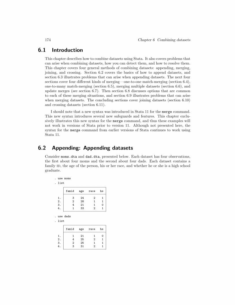
Consider moms.dta and dad.dta, presented below. Each dataset has four observations,the first about four moms and the second about four dads. Each dataset contains afamily ID, the age of the person, his or her race, and whether he or she is a high schoolgraduate.

. use moms

. list

famid age race hs

1. 3 24 2 12. 2 28 1 13. 4 21 1 04. 1 33 2 1

. use dads

. list

famid age race hs

1. 1 21 1 02. 4 25 2 13. 2 25 1 14. 3 31 2 1

6.2 Appending: Appending datasets 175

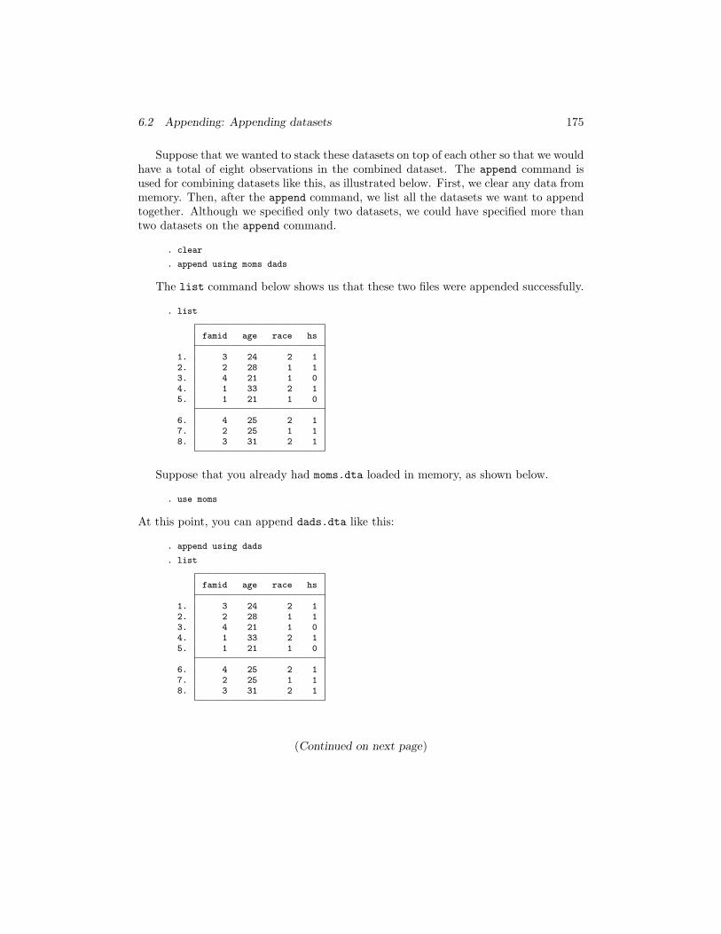
Suppose that we wanted to stack these datasets on top of each other so that we wouldhave a total of eight observations in the combined dataset. The append command isused for combining datasets like this, as illustrated below. First, we clear any data frommemory. Then, after the append command, we list all the datasets we want to appendtogether. Although we specified only two datasets, we could have specified more thantwo datasets on the append command.

. clear

. append using moms dads

The list command below shows us that these two files were appended successfully.

. list

famid age race hs

1. 3 24 2 12. 2 28 1 13. 4 21 1 04. 1 33 2 15. 1 21 1 0

6. 4 25 2 17. 2 25 1 18. 3 31 2 1

Suppose that you already had moms.dta loaded in memory, as shown below.

. use moms

At this point, you can append dads.dta like this:

. append using dads

. list

famid age race hs

1. 3 24 2 12. 2 28 1 13. 4 21 1 04. 1 33 2 15. 1 21 1 0

6. 4 25 2 17. 2 25 1 18. 3 31 2 1

(Continued on next page)

176 Chapter 6 Combining datasets

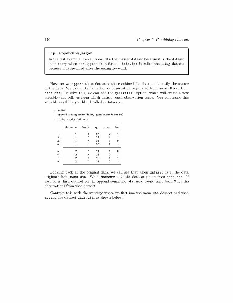
Tip! Appending jargon

In the last example, we call moms.dta the master dataset because it is the datasetin memory when the append is initiated. dads.dta is called the using datasetbecause it is specified after the using keyword.

However we append these datasets, the combined file does not identify the sourceof the data. We cannot tell whether an observation originated from moms.dta or fromdads.dta. To solve this, we can add the generate() option, which will create a newvariable that tells us from which dataset each observation came. You can name thisvariable anything you like; I called it datasrc.

. clear

. append using moms dads, generate(datasrc)

. list, sepby(datasrc)

datasrc famid age race hs

1. 1 3 24 2 12. 1 2 28 1 13. 1 4 21 1 04. 1 1 33 2 1

5. 2 1 21 1 06. 2 4 25 2 17. 2 2 25 1 18. 2 3 31 2 1

Looking back at the original data, we can see that when datasrc is 1, the dataoriginate from moms.dta. When datasrc is 2, the data originate from dads.dta. Ifwe had a third dataset on the append command, datasrc would have been 3 for theobservations from that dataset.

Contrast this with the strategy where we first use the moms.dta dataset and thenappend the dataset dads.dta, as shown below.

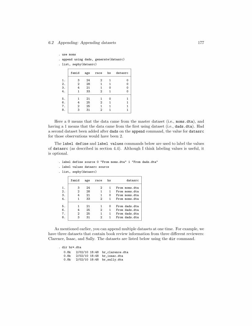
6.2 Appending: Appending datasets 177

. use moms

. append using dads, generate(datasrc)

. list, sepby(datasrc)

famid age race hs datasrc

1. 3 24 2 1 02. 2 28 1 1 03. 4 21 1 0 04. 1 33 2 1 0

5. 1 21 1 0 16. 4 25 2 1 17. 2 25 1 1 18. 3 31 2 1 1

Here a 0 means that the data came from the master dataset (i.e., moms.dta), andhaving a 1 means that the data came from the first using dataset (i.e., dads.dta). Hada second dataset been added after dads on the append command, the value for datasrcfor those observations would have been 2.

The label define and label values commands below are used to label the valuesof datasrc (as described in section 4.4). Although I think labeling values is useful, itis optional.

. label define source 0 "From moms.dta" 1 "From dads.dta"

. label values datasrc source

. list, sepby(datasrc)

famid age race hs datasrc

1. 3 24 2 1 From moms.dta2. 2 28 1 1 From moms.dta3. 4 21 1 0 From moms.dta4. 1 33 2 1 From moms.dta

5. 1 21 1 0 From dads.dta6. 4 25 2 1 From dads.dta7. 2 25 1 1 From dads.dta8. 3 31 2 1 From dads.dta

As mentioned earlier, you can append multiple datasets at one time. For example, wehave three datasets that contain book review information from three different reviewers:Clarence, Isaac, and Sally. The datasets are listed below using the dir command.

. dir br*.dta

0.8k 2/02/10 18:48 br_clarence.dta0.8k 2/02/10 18:48 br_isaac.dta0.8k 2/02/10 18:48 br_sally.dta

178 Chapter 6 Combining datasets

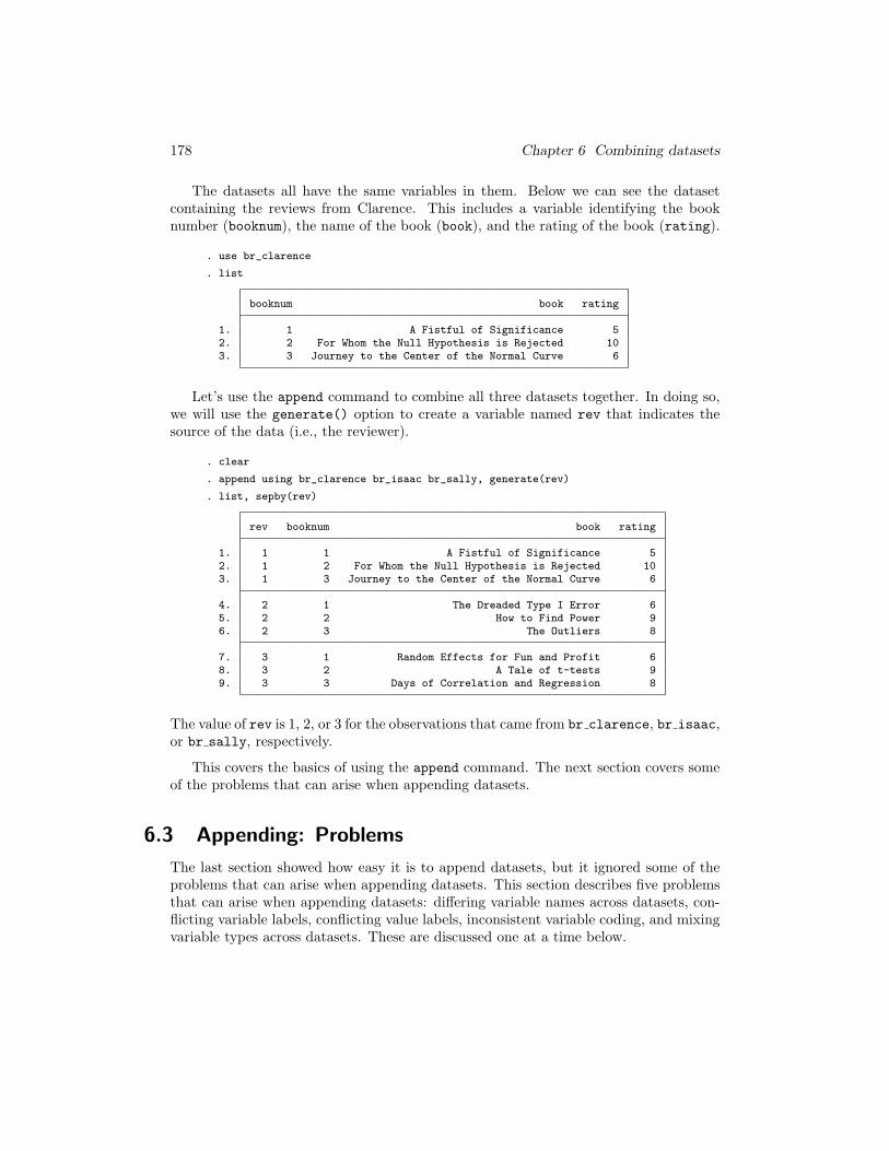
The datasets all have the same variables in them. Below we can see the datasetcontaining the reviews from Clarence. This includes a variable identifying the booknumber (booknum), the name of the book (book), and the rating of the book (rating).

. use br_clarence

. list

booknum book rating

1. 1 A Fistful of Significance 52. 2 For Whom the Null Hypothesis is Rejected 103. 3 Journey to the Center of the Normal Curve 6

Let’s use the append command to combine all three datasets together. In doing so,we will use the generate() option to create a variable named rev that indicates thesource of the data (i.e., the reviewer).

. clear

. append using br_clarence br_isaac br_sally, generate(rev)

. list, sepby(rev)

rev booknum book rating

1. 1 1 A Fistful of Significance 52. 1 2 For Whom the Null Hypothesis is Rejected 103. 1 3 Journey to the Center of the Normal Curve 6

4. 2 1 The Dreaded Type I Error 65. 2 2 How to Find Power 96. 2 3 The Outliers 8

7. 3 1 Random Effects for Fun and Profit 68. 3 2 A Tale of t-tests 99. 3 3 Days of Correlation and Regression 8

The value of rev is 1, 2, or 3 for the observations that came from br clarence, br isaac,or br sally, respectively.

This covers the basics of using the append command. The next section covers someof the problems that can arise when appending datasets.

6.3 Appending: Problems

The last section showed how easy it is to append datasets, but it ignored some of theproblems that can arise when appending datasets. This section describes five problemsthat can arise when appending datasets: differing variable names across datasets, con-flicting variable labels, conflicting value labels, inconsistent variable coding, and mixingvariable types across datasets. These are discussed one at a time below.

6.4 Merging: One-to-one match-merging 189

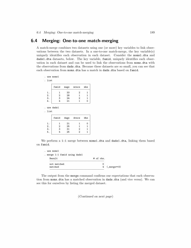
6.4 Merging: One-to-one match-merging

A match-merge combines two datasets using one (or more) key variables to link obser-vations between the two datasets. In a one-to-one match-merge, the key variable(s)uniquely identifies each observation in each dataset. Consider the moms1.dta anddads1.dta datasets, below. The key variable, famid, uniquely identifies each obser-vation in each dataset and can be used to link the observations from moms.dta withthe observations from dads.dta. Because these datasets are so small, you can see thateach observation from moms.dta has a match in dads.dta based on famid.

. use moms1

. list

famid mage mrace mhs

1. 1 33 2 12. 2 28 1 13. 3 24 2 14. 4 21 1 0

. use dads1

. list

famid dage drace dhs

1. 1 21 1 02. 2 25 1 13. 3 31 2 14. 4 25 2 1

We perform a 1:1 merge between moms1.dta and dads1.dta, linking them basedon famid.

. use moms1

. merge 1:1 famid using dads1

Result # of obs.

not matched 0matched 4 (_merge==3)

The output from the merge command confirms our expectations that each observa-tion from moms.dta has a matched observation in dads.dta (and vice versa). We cansee this for ourselves by listing the merged dataset.

(Continued on next page)

190 Chapter 6 Combining datasets

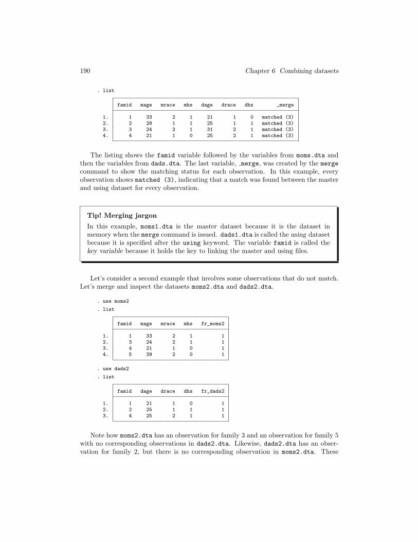
. list

famid mage mrace mhs dage drace dhs _merge

1. 1 33 2 1 21 1 0 matched (3)2. 2 28 1 1 25 1 1 matched (3)3. 3 24 2 1 31 2 1 matched (3)4. 4 21 1 0 25 2 1 matched (3)

The listing shows the famid variable followed by the variables from moms.dta andthen the variables from dads.dta. The last variable, merge, was created by the merge

command to show the matching status for each observation. In this example, everyobservation shows matched (3), indicating that a match was found between the masterand using dataset for every observation.

Tip! Merging jargon

In this example, moms1.dta is the master dataset because it is the dataset inmemory when the merge command is issued. dads1.dta is called the using datasetbecause it is specified after the using keyword. The variable famid is called thekey variable because it holds the key to linking the master and using files.

Let’s consider a second example that involves some observations that do not match.Let’s merge and inspect the datasets moms2.dta and dads2.dta.

. use moms2

. list

famid mage mrace mhs fr_moms2

1. 1 33 2 1 12. 3 24 2 1 13. 4 21 1 0 14. 5 39 2 0 1

. use dads2

. list

famid dage drace dhs fr_dads2

1. 1 21 1 0 12. 2 25 1 1 13. 4 25 2 1 1

Note how moms2.dta has an observation for family 3 and an observation for family 5with no corresponding observations in dads2.dta. Likewise, dads2.dta has an obser-vation for family 2, but there is no corresponding observation in moms2.dta. These

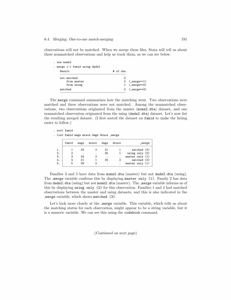
6.4 Merging: One-to-one match-merging 191

observations will not be matched. When we merge these files, Stata will tell us aboutthese nonmatched observations and help us track them, as we can see below.

. use moms2

. merge 1:1 famid using dads2

Result # of obs.

not matched 3from master 2 (_merge==1)from using 1 (_merge==2)

matched 2 (_merge==3)

The merge command summarizes how the matching went. Two observations werematched and three observations were not matched. Among the nonmatched obser-vations, two observations originated from the master (moms2.dta) dataset, and onenonmatched observation originated from the using (dads2.dta) dataset. Let’s now listthe resulting merged dataset. (I first sorted the dataset on famid to make the listingeasier to follow.)

. sort famid

. list famid mage mrace dage drace _merge

famid mage mrace dage drace _merge

1. 1 33 2 21 1 matched (3)2. 2 . . 25 1 using only (2)3. 3 24 2 . . master only (1)4. 4 21 1 25 2 matched (3)5. 5 39 2 . . master only (1)

Families 3 and 5 have data from moms2.dta (master) but not dads2.dta (using).The merge variable confirms this by displaying master only (1). Family 2 has datafrom dads2.dta (using) but not moms2.dta (master). The merge variable informs us ofthis by displaying using only (2) for this observation. Families 1 and 4 had matchedobservations between the master and using datasets, and this is also indicated in themerge variable, which shows matched (3).

Let’s look more closely at the merge variable. This variable, which tells us aboutthe matching status for each observation, might appear to be a string variable, but itis a numeric variable. We can see this using the codebook command.

(Continued on next page)

192 Chapter 6 Combining datasets

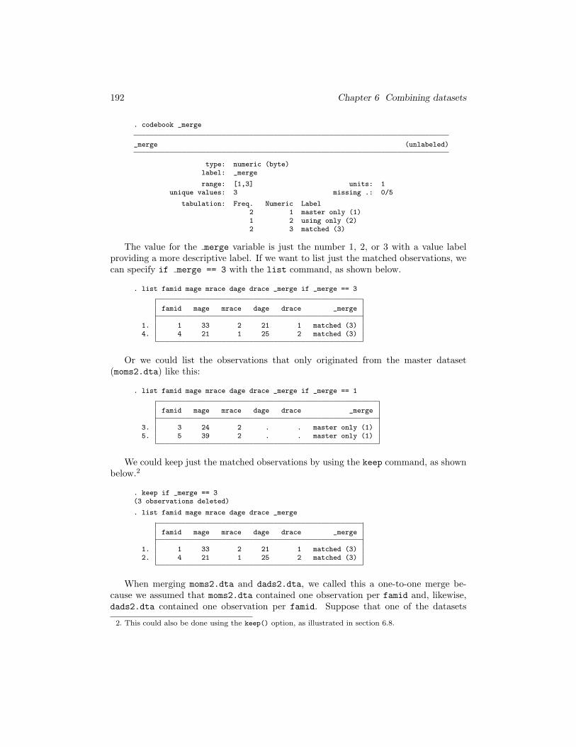
. codebook _merge

_merge (unlabeled)

type: numeric (byte)label: _merge

range: [1,3] units: 1unique values: 3 missing .: 0/5

tabulation: Freq. Numeric Label2 1 master only (1)1 2 using only (2)2 3 matched (3)

The value for the merge variable is just the number 1, 2, or 3 with a value labelproviding a more descriptive label. If we want to list just the matched observations, wecan specify if merge == 3 with the list command, as shown below.

. list famid mage mrace dage drace _merge if _merge == 3

famid mage mrace dage drace _merge

1. 1 33 2 21 1 matched (3)4. 4 21 1 25 2 matched (3)

Or we could list the observations that only originated from the master dataset(moms2.dta) like this:

. list famid mage mrace dage drace _merge if _merge == 1

famid mage mrace dage drace _merge

3. 3 24 2 . . master only (1)5. 5 39 2 . . master only (1)

We could keep just the matched observations by using the keep command, as shownbelow.2

. keep if _merge == 3(3 observations deleted)

. list famid mage mrace dage drace _merge

famid mage mrace dage drace _merge

1. 1 33 2 21 1 matched (3)2. 4 21 1 25 2 matched (3)

When merging moms2.dta and dads2.dta, we called this a one-to-one merge be-cause we assumed that moms2.dta contained one observation per famid and, likewise,dads2.dta contained one observation per famid. Suppose that one of the datasets

2. This could also be done using the keep() option, as illustrated in section 6.8.

6.4 Merging: One-to-one match-merging 193

had more than one observation per famid. momsdup.dta is such a dataset. This valueof famid is accidentally repeated for the last observation (it shows as 4 for the lastobservation but should be 5).

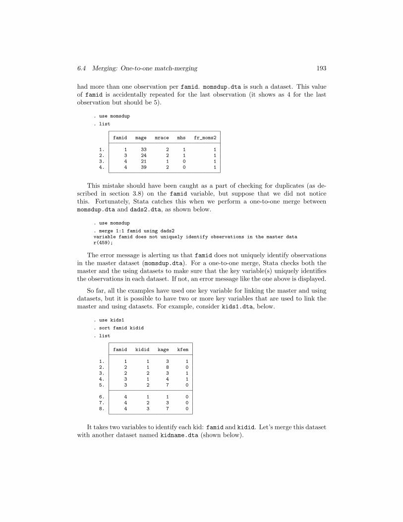
. use momsdup

. list

famid mage mrace mhs fr_moms2

1. 1 33 2 1 12. 3 24 2 1 13. 4 21 1 0 14. 4 39 2 0 1

This mistake should have been caught as a part of checking for duplicates (as de-scribed in section 3.8) on the famid variable, but suppose that we did not noticethis. Fortunately, Stata catches this when we perform a one-to-one merge betweenmomsdup.dta and dads2.dta, as shown below.

. use momsdup

. merge 1:1 famid using dads2variable famid does not uniquely identify observations in the master datar(459);

The error message is alerting us that famid does not uniquely identify observationsin the master dataset (momsdup.dta). For a one-to-one merge, Stata checks both themaster and the using datasets to make sure that the key variable(s) uniquely identifiesthe observations in each dataset. If not, an error message like the one above is displayed.

So far, all the examples have used one key variable for linking the master and usingdatasets, but it is possible to have two or more key variables that are used to link themaster and using datasets. For example, consider kids1.dta, below.

. use kids1

. sort famid kidid

. list

famid kidid kage kfem

1. 1 1 3 12. 2 1 8 03. 2 2 3 14. 3 1 4 15. 3 2 7 0

6. 4 1 1 07. 4 2 3 08. 4 3 7 0

It takes two variables to identify each kid: famid and kidid. Let’s merge this datasetwith another dataset named kidname.dta (shown below).

194 Chapter 6 Combining datasets

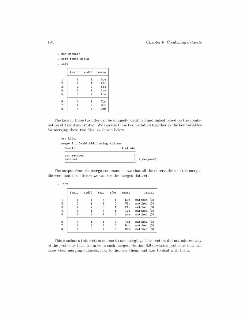
. use kidname

. sort famid kidid

. list

famid kidid kname

1. 1 1 Sue2. 2 1 Vic3. 2 2 Flo4. 3 1 Ivy5. 3 2 Abe

6. 4 1 Tom7. 4 2 Bob8. 4 3 Cam

The kids in these two files can be uniquely identified and linked based on the combi-nation of famid and kidid. We can use these two variables together as the key variablesfor merging these two files, as shown below.

. use kids1

. merge 1:1 famid kidid using kidname

Result # of obs.

not matched 0matched 8 (_merge==3)

The output from the merge command shows that all the observations in the mergedfile were matched. Below we can see the merged dataset.

. list

famid kidid kage kfem kname _merge

1. 1 1 3 1 Sue matched (3)2. 2 1 8 0 Vic matched (3)3. 2 2 3 1 Flo matched (3)4. 3 1 4 1 Ivy matched (3)5. 3 2 7 0 Abe matched (3)

6. 4 1 1 0 Tom matched (3)7. 4 2 3 0 Bob matched (3)8. 4 3 7 0 Cam matched (3)

This concludes this section on one-to-one merging. This section did not address anyof the problems that can arise in such merges. Section 6.9 discusses problems that canarise when merging datasets, how to discover them, and how to deal with them.

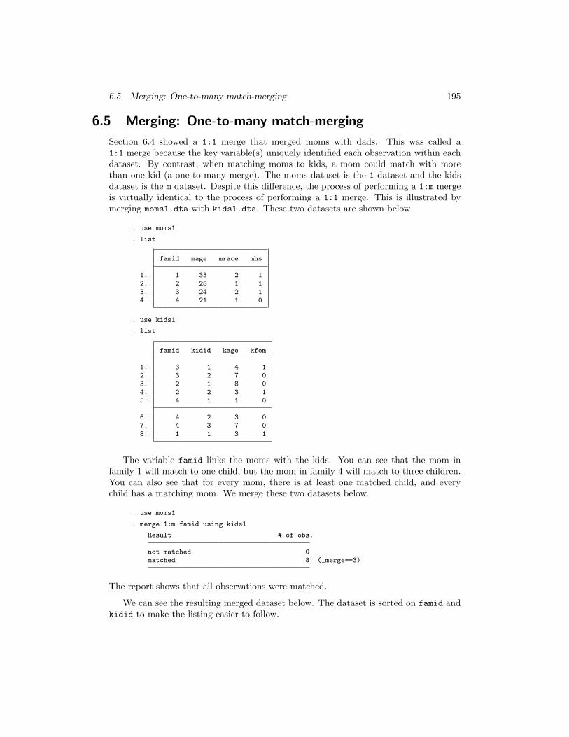
6.5 Merging: One-to-many match-merging 195

6.5 Merging: One-to-many match-merging

Section 6.4 showed a 1:1 merge that merged moms with dads. This was called a1:1 merge because the key variable(s) uniquely identified each observation within eachdataset. By contrast, when matching moms to kids, a mom could match with morethan one kid (a one-to-many merge). The moms dataset is the 1 dataset and the kidsdataset is the m dataset. Despite this difference, the process of performing a 1:m mergeis virtually identical to the process of performing a 1:1 merge. This is illustrated bymerging moms1.dta with kids1.dta. These two datasets are shown below.

. use moms1

. list

famid mage mrace mhs

1. 1 33 2 12. 2 28 1 13. 3 24 2 14. 4 21 1 0

. use kids1

. list

famid kidid kage kfem

1. 3 1 4 12. 3 2 7 03. 2 1 8 04. 2 2 3 15. 4 1 1 0

6. 4 2 3 07. 4 3 7 08. 1 1 3 1

The variable famid links the moms with the kids. You can see that the mom infamily 1 will match to one child, but the mom in family 4 will match to three children.You can also see that for every mom, there is at least one matched child, and everychild has a matching mom. We merge these two datasets below.

. use moms1

. merge 1:m famid using kids1

Result # of obs.

not matched 0matched 8 (_merge==3)

The report shows that all observations were matched.

We can see the resulting merged dataset below. The dataset is sorted on famid andkidid to make the listing easier to follow.