16.90 Project 1

Spring 2014

1 Problem 1

Introduction

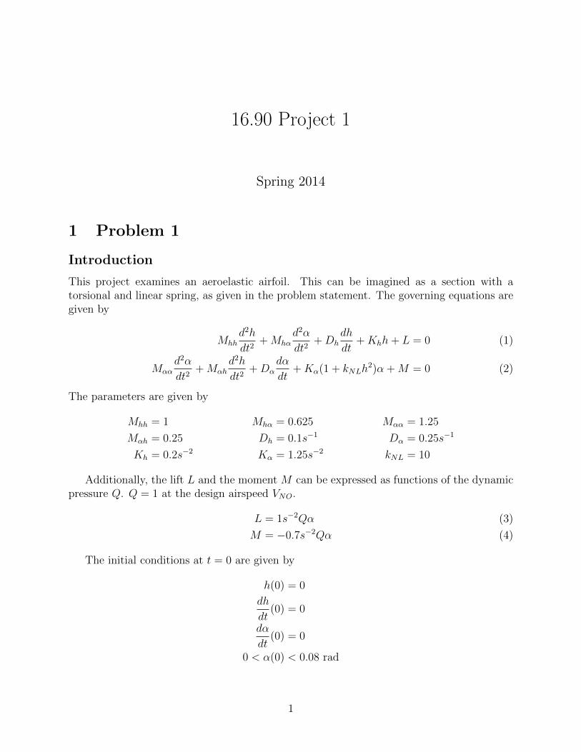
This project examines an aeroelastic airfoil. This can be imagined as a section with atorsional and linear spring, as given in the problem statement. The governing equations aregiven by

d2hMhh

dt2+Mhα

d2α

dt2+Dh

dh

dt+Khh+ L = 0 (1)

Mααd2α d2h

+Mαhdt2 dt2

+Dαdα

+K 2α(1 + kNLh )α +M = 0 (2)

dt

The parameters are given by

Mhh = 1 Mhα = 0.625 Mαα = 1.25

Mαh = 0.25 Dh = 0.1s−1 Dα = 0.25s−1

Kh = 0.2s−2 Kα = 1.25s−2 kNL = 10

Additionally, the lift L and the moment M can be expressed as functions of the dynamicpressure Q. Q = 1 at the design airspeed VNO.

L = 1s−2Qα (3)

M = −0.7s−2Qα (4)

The initial conditions at t = 0 are given by

h(0) = 0

dh(0) = 0

dtdα

(0) = 0dt

0 < α(0) < 0.08 rad

1

1.1

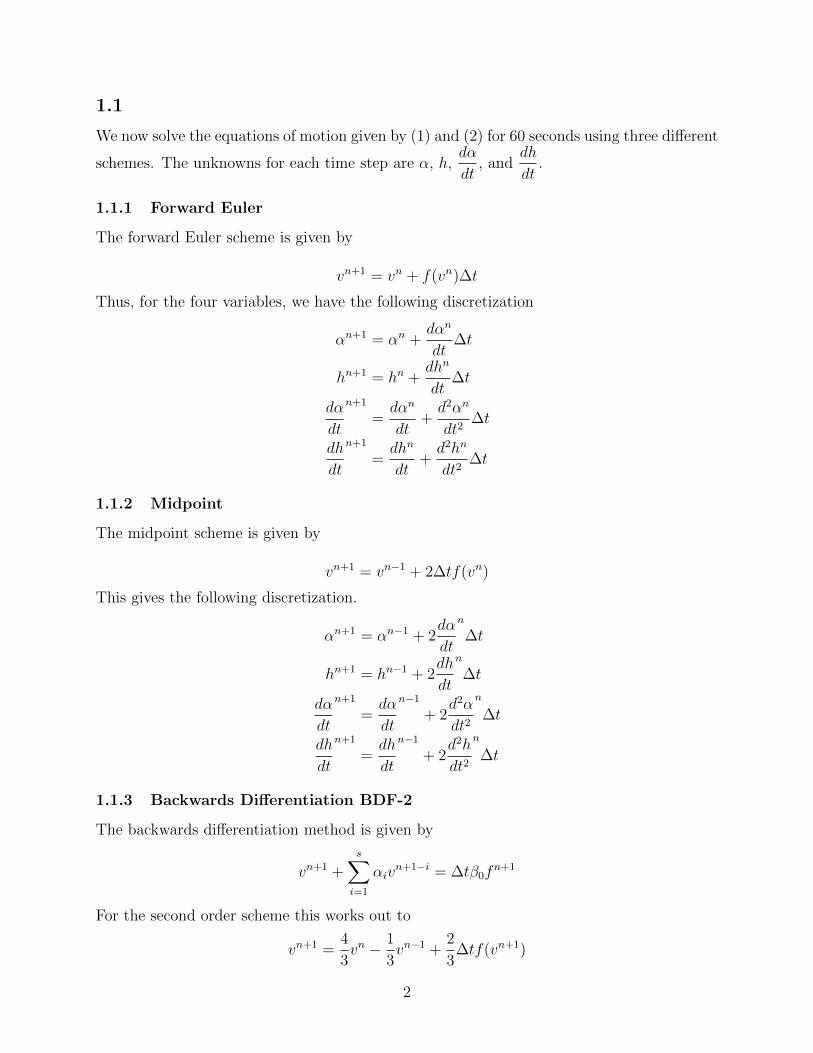
We now solve the equations of motion given by (1) and (2) for 60 seconds using three differentdα

schemes. The unknowns for each time step are α, h,dt

, anddh

.dt

1.1.1 Forward Euler

The forward Euler scheme is given by

vn+1 = vn + f(vn)∆t

Thus, for the four variables, we have the following discretization

n

αn+1 = αndα

+dt

∆t

hn+1 = hn +dhn

∆tdt

dαn+1 dαn=

dt dt+d2αn

dt2∆t

dh

dt

n+1

=dhn

dt+d2hn

∆tdt2

1.1.2 Midpoint

The midpoint scheme is given by

vn+1 = vn−1 + 2∆tf(vn)

This gives the following discretization.

αn+1 dα= αn−1 + 2

n

∆tdt

hn+1 = hn−1 dh+ 2

dt

n

∆t

dα

dt

n+1

=dαn−1 d2α

+ 2dt dt2

n

∆t

dh

dt

n+1

=dh

dt

n−1

+ 2d2h

n

∆tdt2

1.1.3 Backwards Differentiation BDF-2

The backwards differentiation method is given by

s

vn+1 +∑

αivn+1−i = ∆tβ0f

n+1

i=1

For the second order scheme this works out to

vn+1 4=

3vn − 1

3vn−1 +

2∆tf(vn+1)

3

2

4 n+1n+1 = αn

1α − αn−1 2 dα

+ ∆t3 3 3 dt

hn+1 4 +1

= hn1 n

− hn2−1 dh

+ ∆t3 3 3 dt

dαn+1 4 dαn 1 dαn−1 2 d2n+1

α= + ∆t

dt 3 dt−

3 dt 3 dt2

dhn+1 4 dhn 1 n−1 d2n+1

dh 2 h= +

dt 3 dt− ∆t

3 dt 3 dt2

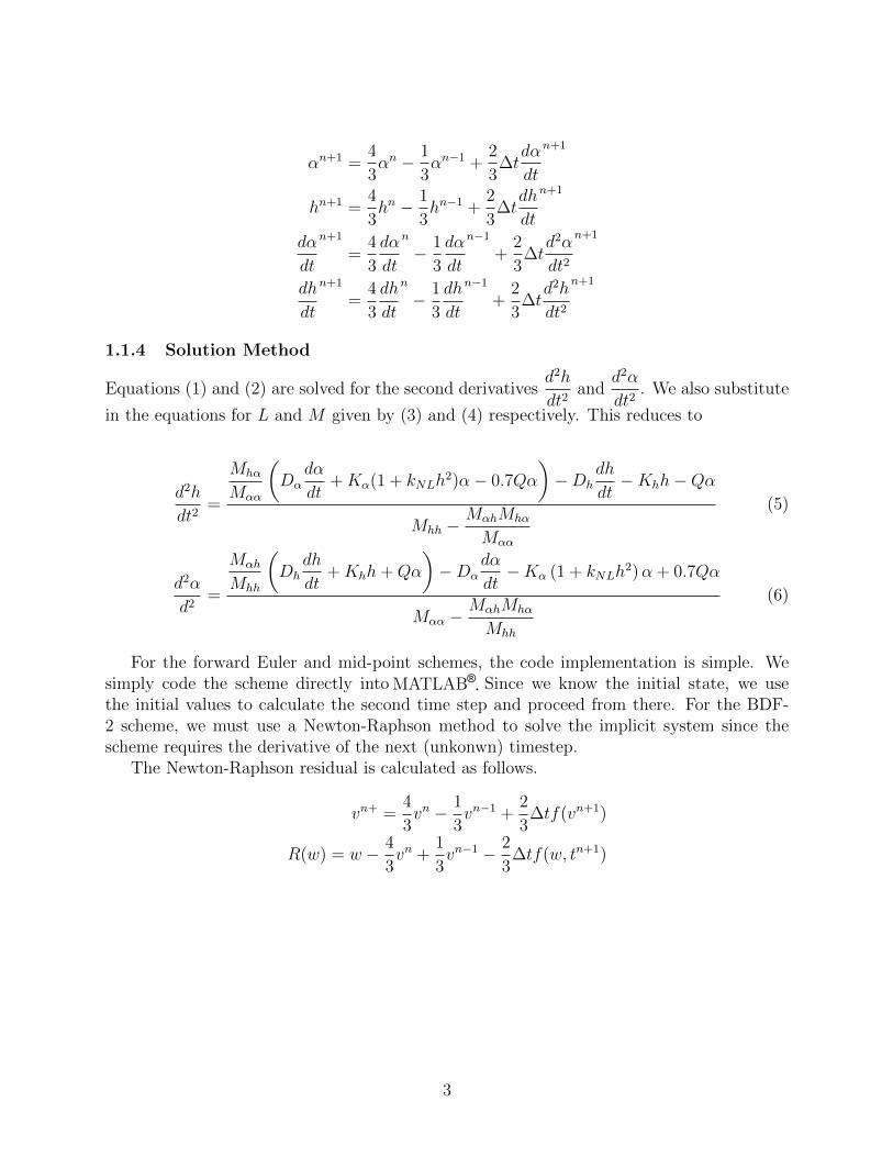
1.1.4 Solution Method

d2h d2αEquations (1) and (2) are solved for the second derivatives and . We also substitute

dt2 dt2in the equations for L and M given by (3) and (4) respectively. This reduces to

Mhα dα2

(Dα +Kα(1 + kNLh

2)α− 0.7Qα

)dh−Dh K

d h−Qα

Mαα dt dt− hh

= (5)dt2 M

Mhh − αhMhα

Mαα

Mαh dh dα2

(Dh +Khh+Qα D + h2α Kα (1 kNL )α + 0.7Qα

d α Mhh dt

)−

dt−

= (6)d2 M M

Mαα − αh hα

Mhh

For the forward Euler and mid-point schemes, the code implementation is simple. Wesimply code the scheme directly into Since we know the initial state, we usethe initial values to calculate the second time step and proceed from there. For the BDF-2 scheme, we must use a Newton-Raphson method to solve the implicit system since thescheme requires the derivative of the next (unkonwn) timestep.

The Newton-Raphson residual is calculated as follows.

4vn+ = vn

1

3− vn−1 2

+ ∆tf(vn+1)3 3

4 1 2R(w) = w − vn + vn−1

3 3− ∆tf(w, tn+1)

3

3

MATLAB®.

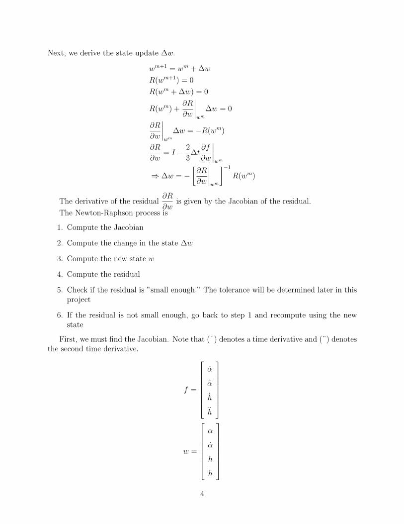
Next, we derive the state update ∆w.

wm+1 = wm + ∆w

R(wm+1) = 0

R(wm + ∆w) = 0

R(wm∂R

) +∂w

∣∆w = 0

wm

∂R∣∣∣∣ ∆w =

∣∣∣−R(wm)

∂w wm

∂R 2 ∂f= I ∆t

∂w−

3 ∂w

∣∣∣∣w

⇒ ∆w = −[∂R

∂w

∣∣ m

wm

]−1

R(wm)

∂RThe derivative of the residual is given b

∂

∣∣y the Jacobian of the residual.

wThe Newton-Raphson process is

1. Compute the Jacobian

2. Compute the change in the state ∆w

3. Compute the new state w

4. Compute the residual

5. Check if the residual is ”small enough.” The tolerance will be determined later in thisproject

6. If the residual is not small enough, go back to step 1 and recompute using the newstate

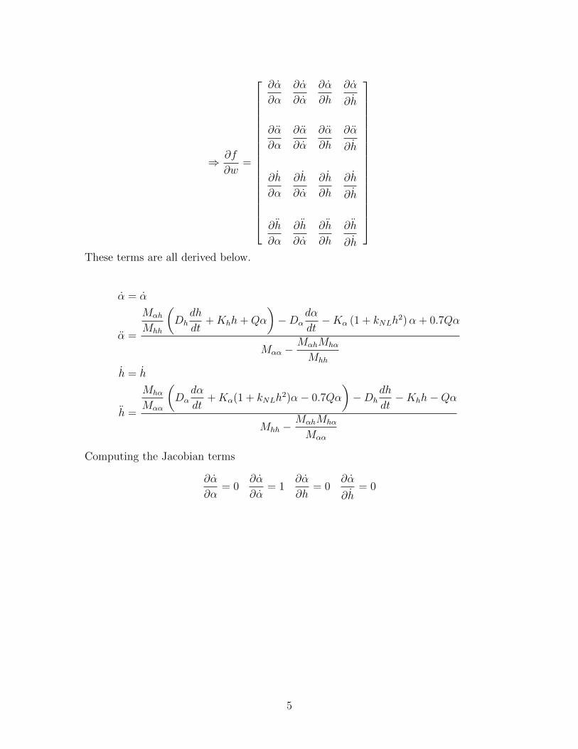
First, we must find the Jacobian. Note that ( ˙ ) denotes a time derivative and (¨) denotesthe second time derivative.

f =

α α

h

¨

h

w =

α

α

h

˙

h

4

∂α ∂α ∂α ∂α ∂α ∂α ∂h ˙ ∂h

∂f=

∂α ∂α ∂α ∂α ∂α ∂α ∂h ˙∂h

⇒

∂w

˙ ˙ ˙ ˙ ∂h ∂h ∂h ∂h

∂α ∂α ∂h ˙

∂h

¨ ¨ ¨ ¨∂h ∂h ∂h ∂h

∂α ∂α ∂h ˙

∂h

These terms are all derived below.

α = α

Mαh

(dh dα

Dh +Khh+Qα

)−Dα −Kα (1 + k 2

NLh )α + 0.7QαMhh dt dt

α =M M

Mαα − αh hα

Mhh

˙ ˙h = h

Mhα

(dα dh

Dα +K 2α(1 + kNLh )α 0.7Qα Dh Khh Qα

M dt dt¨ αα

− −h

)− −

=MαhM− hα

MhhMαα

Computing the Jacobian terms

∂α ∂α ∂α ∂α= 0 = 1 = 0 = 0

∂α ∂α ∂h ˙∂h

5

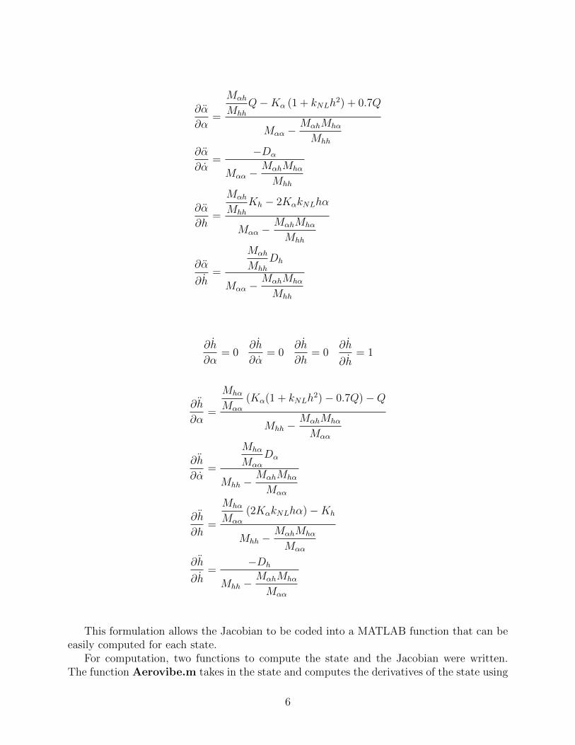
MαhQ−Kα (1 + kNLh

2) + 0.7Q∂α M

= hh

∂α MMαα − αhMhα

Mhh

∂α=

−Dα

∂α MMαα − αhMhα

Mhh

MαhK K

∂α hMhh

− 2 αkNLhα=

∂h M MMαα − αh hα

Mhh

MαhD

∂α hM

= hh

˙∂h M− αhMhαMαα

Mhh

˙ ˙ ˙ ˙∂h ∂h ∂h ∂h= 0 = 0 = 0 = 1

∂α ∂α ∂h ˙∂h

Mhα(K h2)¨∂h α(1 + kNL

Mαα

− 0.7Q)−Q=

∂α MMhh − αhMhα

Mαα

MhαD¨∂h α

M= αα

∂α MαhM− hαMhh

Mαα

Mhα(2K¨∂h αkNLhα)

M= αα

−Kh

∂h MMhh − αhMhα

Mαα

¨∂h −Dh=

˙∂h MMhh − αhMhα

Mαα

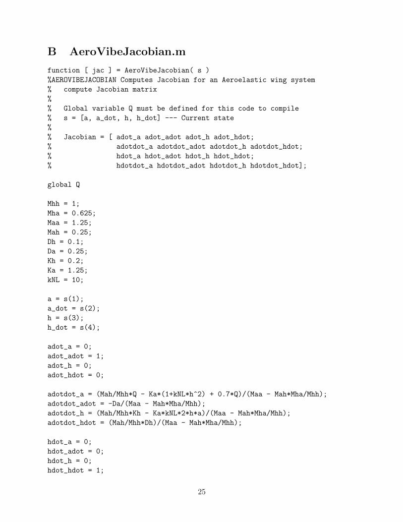
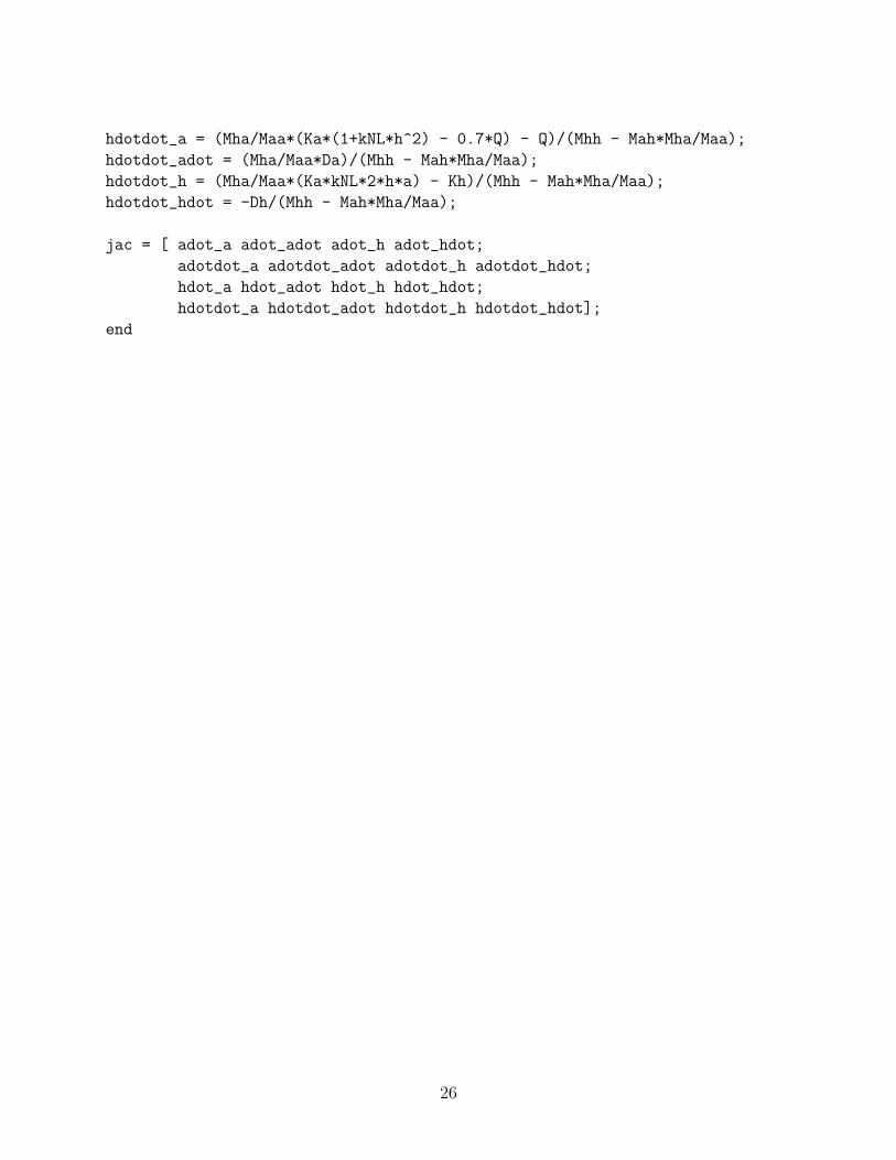
This formulation allows the Jacobian to be coded into a MATLAB function that can beeasily computed for each state.

For computation, two functions to compute the state and the Jacobian were written.The function Aerovibe.m takes in the state and computes the derivatives of the state using

6

equations (5) and (6) for the second derivatives of α and h and dαdt

= α and dh ˙= h for thedt

˙first derivatives. Here, α and h are the current state derivatives. AeroVibeJacobian.muses the equations listed on page 6 to compute the Jacobian of the aeroelastic wing model.See the appendix A for the printout of the code for these two functions.

To compute the schemes, a general function was written for each one. These are attachedin the appendix as well.

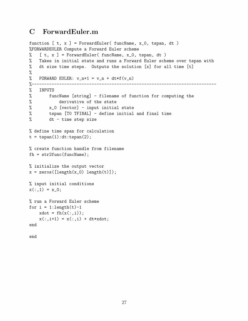
To compute the forward Euler solution, the function ForwardEuler.m takes in thefunction name of the ODE being examined, the timespan vector, the initial state, and thetime step ∆t. It then uses a for loop to compute the forward Euler solution. The ODEfunction computes the derivatives of the state.

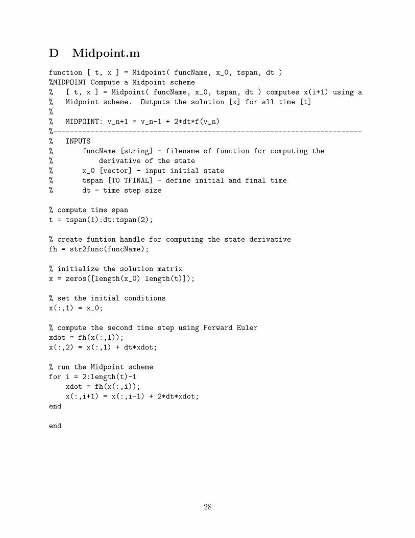
To compute the mid-point solution, a function similar to the forward Euler one is used.Midpoint.m takes in the ODE computation function, the initial state, the time span, andthe time step size. The midpoint function computes the v2 state using a forward Eulerscheme and then computes all subsequent vn using the midpoint scheme.

For the Backward Difference scheme, the function BDF2.m takes in the ODE functionname, the Jacobian function name, the initial state, the time span, the timestep size dt, andthe tolerance. As outlined on page 4, BDF2.m uses a Newton-Raphson scheme to solve theimplicit function. First, v2 is computed using the forward Euler scheme. Then, for each timestep, the process from page 4 is used. Once the desired tolerance is reached vn+1 is set to

∂Rw and the code moves on to the next time step. The Jacobian computed

∂

∣is

f

∣∣∣ by usingw

the Jacobian function used in the input to BDF.m, and the derivative is computed by theODE function.

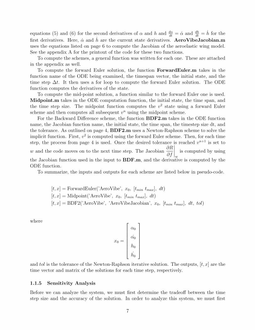
To summarize, the inputs and outputs for each scheme are listed below in pseudo-code.

[t, x] = ForwardEuler(’AeroVibe’, x0, [tmin tmax], dt)

[t, x] = Midpoint(’AeroVibe’, x0, [tmin tmax], dt)

[t, x] = BDF2(’AeroVibe’, ’AeroVibeJacobian’, x0, [tmin tmax], dt, tol)

where x0 =

α0 α0 h0

˙

h0

and tol is the tolerance of the Newton-Raphson iterativ

e solution. The outputs, [t, x] are the

time vector and matrix of the solutions for each time step, respectively.

1.1.5 Sensitivity Analysis

Before we can analyze the system, we must first determine the tradeoff between the timestep size and the accuracy of the solution. In order to analyze this system, we must first

7

pick a baseline with which we can compare various values of dt and their solutions. In orderto do this, we choose to use the BDF-2 scheme. Since it is implicit and this is a non-linearsystem, we assume that it will be the most accurate. We now set about proving it.

First, we pick a ”very small” value for ∆t and the tolerance of the BDF-2 Newton iterationloop. After a small amount of trial and error, we pick ∆t = 10−6 and a tolerance of 10−8.Both of these values are quite small and result in a 1+ hour computation time. We thensave the values of the output for Q = 1 and Q = 1.5 in order to compare the other schemeswith them.

To do the sensitivity analysis, we run a series of trials with each scheme for an array ofvalues of ∆t. These values of ∆t are all an order of magnitude different from each other.For each timestep size and each value of Q we compute the solution and find the maximumerror. This is done by subtracting the most accurate solution from the scheme solution andtaking the absolute value.

Succinctly the process is as follows:

1. Choose scheme

2. Choose ∆t

3. Compute solution for Q = 1 and Q = 1.5

4. Find the maximum, |scheme solution − most accurate|

5. Save the maximum error for h and α and plot the results

For each analysis, the dt vector was

dt = [10−2 10−3 10−4 10−5]

The initial α0 was 0.08.The results show the accuracy of each scheme. By examining the slope of the dt versus

error lines, we can find the order of accuracy. The results for the forward Euler schemesensitivity analysis are shown below.

8

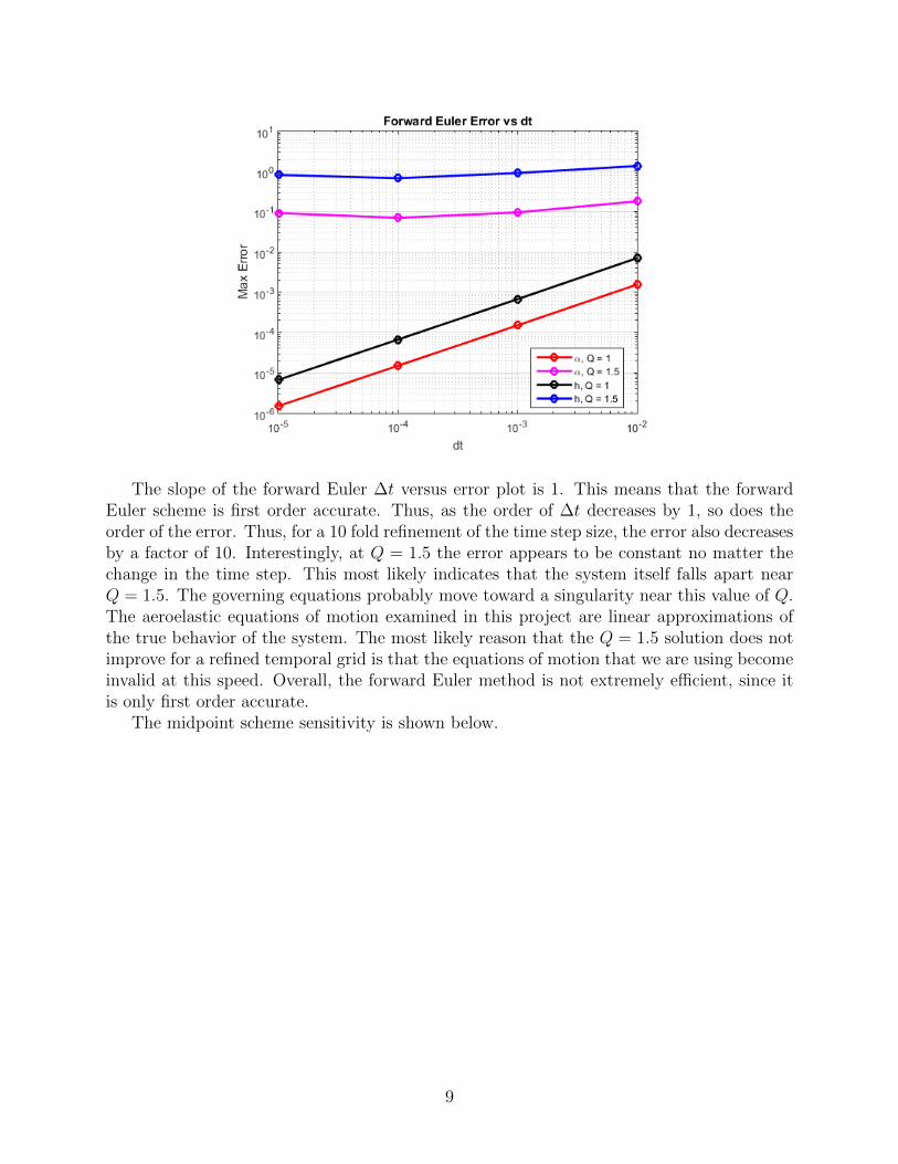
The slope of the forward Euler ∆t versus error plot is 1. This means that the forwardEuler scheme is first order accurate. Thus, as the order of ∆t decreases by 1, so does theorder of the error. Thus, for a 10 fold refinement of the time step size, the error also decreasesby a factor of 10. Interestingly, at Q = 1.5 the error appears to be constant no matter thechange in the time step. This most likely indicates that the system itself falls apart nearQ = 1.5. The governing equations probably move toward a singularity near this value of Q.The aeroelastic equations of motion examined in this project are linear approximations ofthe true behavior of the system. The most likely reason that the Q = 1.5 solution does notimprove for a refined temporal grid is that the equations of motion that we are using becomeinvalid at this speed. Overall, the forward Euler method is not extremely efficient, since itis only first order accurate.

The midpoint scheme sensitivity is shown below.

9

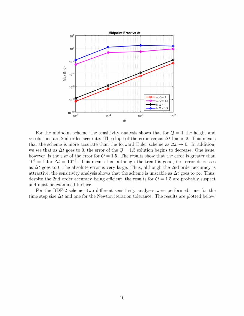
For the midpoint scheme, the sensitivity analysis shows that for Q = 1 the height andα solutions are 2nd order accurate. The slope of the error versus ∆t line is 2. This meansthat the scheme is more accurate than the forward Euler scheme as ∆t → 0. In addition,we see that as ∆t goes to 0, the error of the Q = 1.5 solution begins to decrease. One issue,however, is the size of the error for Q = 1.5. The results show that the error is greater than100 = 1 for ∆t = 10−4. This means that although the trend is good, i.e. error decreasesas ∆t goes to 0, the absolute error is very large. Thus, although the 2nd order accuracy isattractive, the sensitivity analysis shows that the scheme is unstable as ∆t goes to∞. Thus,despite the 2nd order accuracy being efficient, the results for Q = 1.5 are probably suspectand must be examined further.

For the BDF-2 scheme, two different sensitivity analyses were performed: one for thetime step size ∆t and one for the Newton iteration tolerance. The results are plotted below.

10

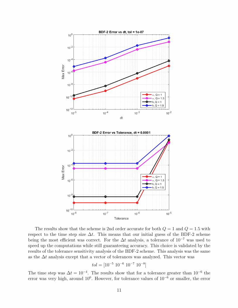
The results show that the scheme is 2nd order accurate for both Q = 1 and Q = 1.5 withrespect to the time step size ∆t. This means that our initial guess of the BDF-2 schemebeing the most efficient was correct. For the ∆t analysis, a tolerance of 10−7 was used tospeed up the computations while still guaranteeing accuracy. This choice is validated by theresults of the tolerance sensitivity analysis of the BDF-2 scheme. This analysis was the sameas the ∆t analysis except that a vector of tolerances was analyzed. This vector was

tol = [10−5 10−6 10−7 10−8]

The time step was ∆t = 10−4. The results show that for a tolerance greater than 10−6 theerror was very high, around 100. However, for tolerance values of 10−6 or smaller, the error

11

was constant. These results show that for the BDF-2 scheme, there is a tolerance for whichthe scheme becomes most accurate for a specific value of ∆t. If the tolerance is decreased,there is no benefit in the error. The error remains constant but computation time increasessubstantially for smaller values of the tolerance. Thus, this is an efficient scheme. We obtain2 order of accuracy for 1 order of loss in efficiency (∆t).

Using the results of the sensitivity analysis, the following parameters were used to calcu-late the solution.

max error from sensitivity analysisscheme ∆t tolerance

Q = 1.0 Q = 1.5

Forward Euler 1e− 4 N/A 10−4 100

Midpoint 1e− 5 N/A 10−8 10−2

BDF-2 1e− 4 1e− 6 10−8 10−4

hese choices of ∆t reflect the values of ∆t which resulted in the least error for Q = 1.5Twhile still trying to keep the code running quickly. For the forward Euler scheme, theminimum error was obtained when ∆t = 10−4. Therefore, since computation time for thistime step size was tolerable, this choice was the logical one. For this choice of ∆t we expectthe following error.

Q = 1 Q = 1.5

α 1.05× 10−5 1.6× 10−2

h 1.6× 10−5 1.5× 10−1

For the midpoint scheme, the choice of ∆t again is limited by the error by the Q = 1.5case. The sensitivity analysis showed that the error for Q = 1.5 was above 10−1 for all∆t ≥ 10−4. Therefore, the only way to obtain an accurate solution is to reduce the timestep size. The tradeoff here is the computation time. A ∆t of 10−5 takes 10 times as manycomputations as a ∆t of 10−4. Therefore, we get an accuracy that we desire but at a lowefficiency. We expect the following errors for ∆t = 10−5 for the midpoint scheme.

Q = 1 Q = 1.5

α 1.4× 10−9 1.2× 10−3

h 1.0× 10−8 1.0× 10−2

For the BDF-2 scheme, the choice of ∆t is much easier. Since a ∆t of 10−3 already has amaximum error of 10−2 for Q = 1.5, which is the same as the error for the midpoint schemeat ∆t = 10−5, the BDF-2 choice is much easier. The same is true for the tolerance value.The analysis showed that for ∆t = 10−4 a tolerance of 10−6 or smaller results in the same

12

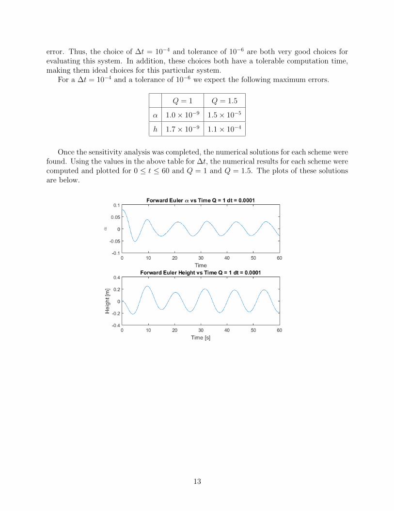
error. Thus, the choice of ∆t = 10−4 and tolerance of 10−6 are both very good choices forevaluating this system. In addition, these choices both have a tolerable computation time,making them ideal choices for this particular system.

For a ∆t = 10−4 and a tolerance of 10−6 we expect the following maximum errors.

Q = 1 Q = 1.5

α 1.0× 10−9 1.5× 10−5

h 1.7× 10−9 1.1× 10−4

Once the sensitivity analysis was completed, the numerical solutions for each scheme werefound. Using the values in the above table for ∆t, the numerical results for each scheme werecomputed and plotted for 0 ≤ t ≤ 60 and Q = 1 and Q = 1.5. The plots of these solutionsare below.

13

14

15

We see from the numerical solutions that for all three schemes for the Q = 1 case thesolution for both α and h are almost identical. This is as expected since we chose ∆t and thetolerance such that the error should be at most 10−4 between the three schemes. Thereforeall three schemes are good methods for the Q = 1 case.

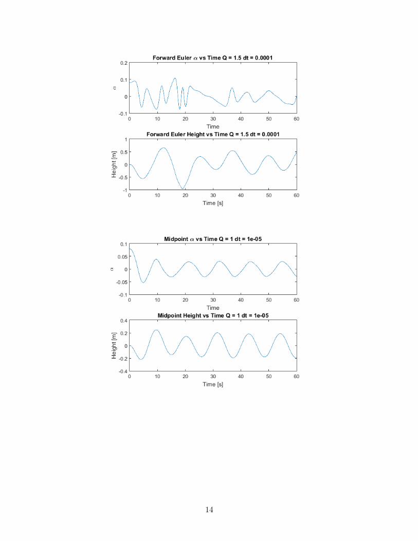
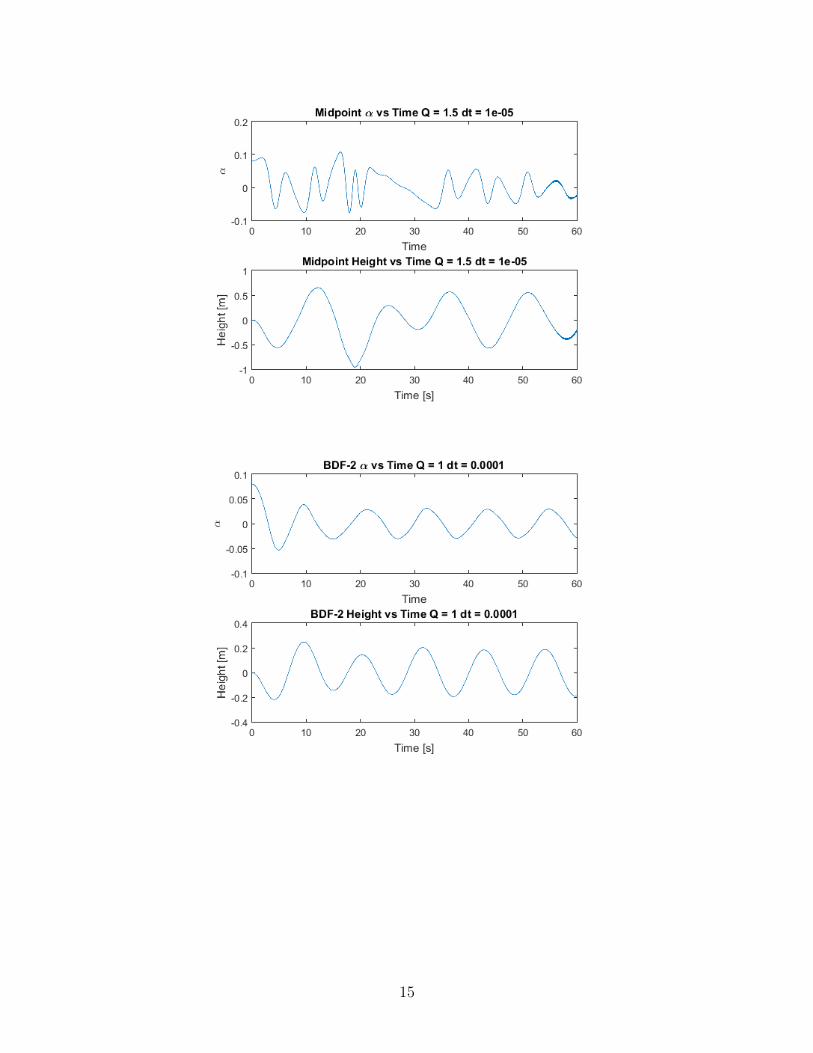
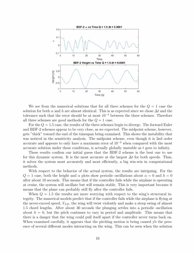
For the Q = 1.5 case, the results of the three schemes begin to diverge. The forward Eulerand BDF-2 schemes appear to be very close, as we expected. The midpoint scheme, however,gets ”thick” toward the end of the timespan being examined. This shows the instability thatwas noticed in the sensitivity analysis. The midpoint scheme, even though it is 2nd orderaccurate and appears to only have a maximum error of 10−2 when compared with the mostaccurate solution under these conditions, is actually globally unstable as t goes to infinity.

These results confirm our initial guess that the BDF-2 scheme is the best one to usefor this dynamic system. It is the most accurate at the largest ∆t for both speeds. Thus,it solves the system most accurately and most efficiently, a big win-win in computationalmethods.

With respect to the behavior of the actual system, the results are intriguing. For theQ = 1 case, both the height and α plots show periodic oscillations about α = 0 and h = 0after about 10 seconds. This means that if the controller fails while the airplane is operatingat cruise, the system will oscillate but will remain stable. This is very important because itmeans that the plane can probably still fly after the controller fails.

When Q = 1.5 the results are more worrying with respect to the wing’s structural in-tegrity. The numerical models predict that if the controller fails while the airplane is flying atthe never-exceed speed, VNE, the wing will twist violently and make a steep swing of almost1.5 chord lengths. After about 30 seconds the plunging settles into a periodic oscillationabout h = 0, but the pitch continues to vary in period and amplitude. This means thatthere is a danger that the wing could pull itself apart if the controller never turns back on.When examined carefully, it appears that the pitching motion is being caused yb the pres-ence of several different modes interacting on the wing. This can be seen when the solution

16

becomes almost a straight line around t = 30, but then quickly becomes oscillatory againapproximately 5 seconds later. This behavior suggests presence of a few different eigenmodesin the system. This would also explain the oscillatory nature of the solutions.

In summary, we find through our analysis that the BDF-2 scheme is the most efficientand the most accurate scheme for solving this system.

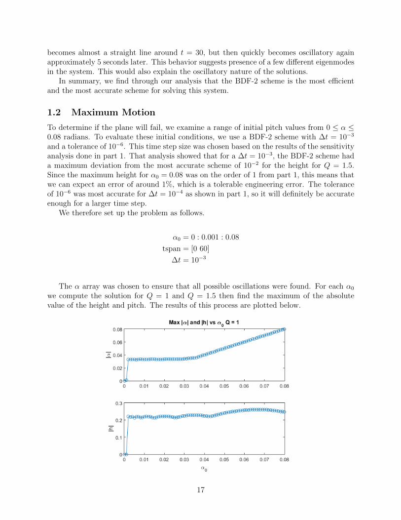
1.2 Maximum Motion

To determine if the plane will fail, we examine a range of initial pitch values from 0 ≤ α ≤0.08 radians. To evaluate these initial conditions, we use a BDF-2 scheme with ∆t = 10−3

and a tolerance of 10−6. This time step size was chosen based on the results of the sensitivityanalysis done in part 1. That analysis showed that for a ∆t = 10−3, the BDF-2 scheme hada maximum deviation from the most accurate scheme of 10−2 for the height for Q = 1.5.Since the maximum height for α0 = 0.08 was on the order of 1 from part 1, this means thatwe can expect an error of around 1%, which is a tolerable engineering error. The toleranceof 10−6 was most accurate for ∆t = 10−4 as shown in part 1, so it will definitely be accurateenough for a larger time step.

We therefore set up the problem as follows.

α0 = 0 : 0.001 : 0.08

tspan = [0 60]

∆t = 10−3

The α array was chosen to ensure that all possible oscillations were found. For each α0

we compute the solution for Q = 1 and Q = 1.5 then find the maximum of the absolutevalue of the height and pitch. The results of this process are plotted below.

17

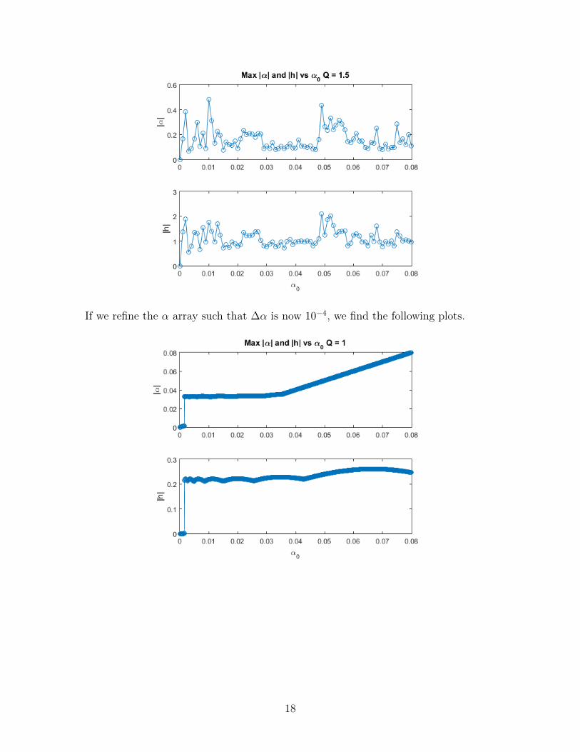
If we refine the α array such that ∆α is now 10−4, we find the following plots.

18

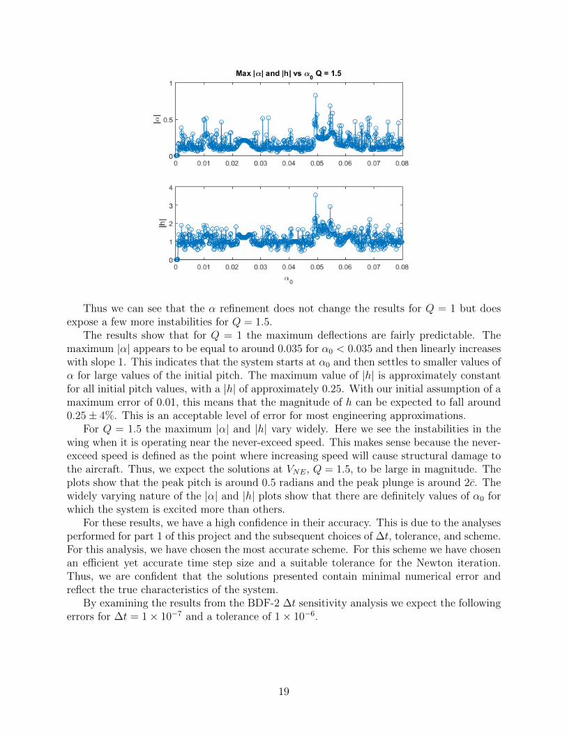
Thus we can see that the α refinement does not change the results for Q = 1 but doesexpose a few more instabilities for Q = 1.5.

The results show that for Q = 1 the maximum deflections are fairly predictable. Themaximum |α| appears to be equal to around 0.035 for α0 < 0.035 and then linearly increaseswith slope 1. This indicates that the system starts at α0 and then settles to smaller values ofα for large values of the initial pitch. The maximum value of |h| is approximately constantfor all initial pitch values, with a |h| of approximately 0.25. With our initial assumption of amaximum error of 0.01, this means that the magnitude of h can be expected to fall around0.25± 4%. This is an acceptable level of error for most engineering approximations.

For Q = 1.5 the maximum |α| and |h| vary widely. Here we see the instabilities in thewing when it is operating near the never-exceed speed. This makes sense because the never-exceed speed is defined as the point where increasing speed will cause structural damage tothe aircraft. Thus, we expect the solutions at VNE, Q = 1.5, to be large in magnitude. Theplots show that the peak pitch is around 0.5 radians and the peak plunge is around 2c. Thewidely varying nature of the |α| and |h| plots show that there are definitely values of α0 forwhich the system is excited more than others.

For these results, we have a high confidence in their accuracy. This is due to the analysesperformed for part 1 of this project and the subsequent choices of ∆t, tolerance, and scheme.For this analysis, we have chosen the most accurate scheme. For this scheme we have chosenan efficient yet accurate time step size and a suitable tolerance for the Newton iteration.Thus, we are confident that the solutions presented contain minimal numerical error andreflect the true characteristics of the system.

By examining the results from the BDF-2 ∆t sensitivity analysis we expect the followingerrors for ∆t = 1× 10−7 and a tolerance of 1× 10−6.

19

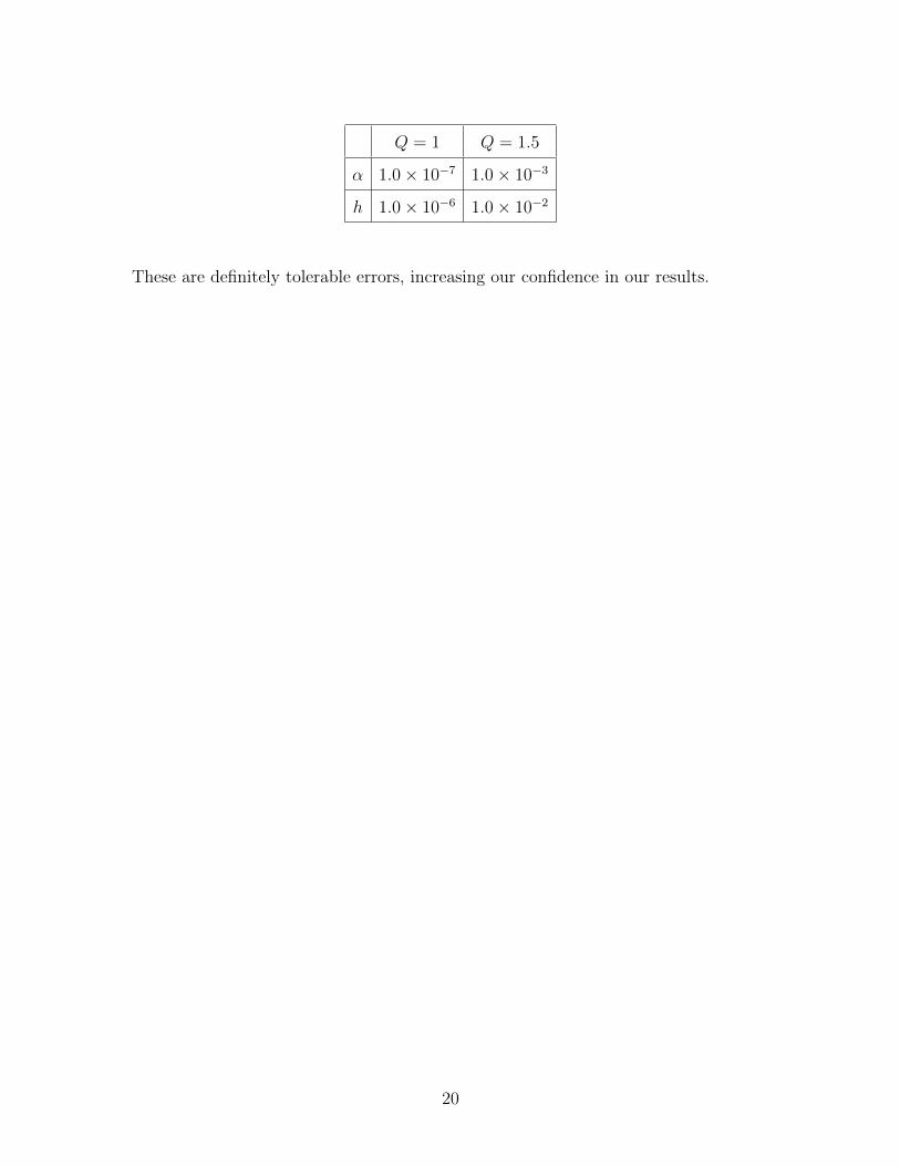
Q = 1 Q = 1.5

α 1.0× 10−7 1.0× 10−3

h 1.0× 10−6 1.0× 10−2

These are definitely tolerable errors, increasing our confidence in our results.

20

2 Problem 2

We now examine an advection system. The governing equation is given by

∂u

∂t=∂cx(x, y)u ∂cy(x, y)u

+∂x

(7)∂y

(8)

where u(x, y, t) is the density, cx(x, y) is the flow field in the x direction, and cy(x, y) is theflow field in the y direction.

We solve this equation over the domain 0 ≤ x ≤ 1 and 0 ≤ y ≤ 1. The boundaryconditions are given by

u(x, y, 0) = 0

u(0, y, t) = u(x, 0, t) = sin(πt)

We use a Forward Time, Backward Space (FTBS) method to solve this system. TheBackward Space discretization gives

∂Un

∂x

∣∣∣ cxUn∣ i,j

=− cxUn

i−1,j

i,j ∆x(9)

∂U

∂y

∣∣∣∣ni,j

=cyU

ni,j − cyUn

i,j−1(10)

∆y

The Forward Time discretization is given by

∂U

∂t

∣∣∣∣ni,j

=Un+1i,j − Un

i,j(11)

∆t

For these equations ∆x = ∆y = 1/512 and ∆t = 1/1024 as defined in the problemstatement.

We now set about implementing this scheme. We start with the baseline code that wasgiven with the problem statement. This code loads cx, cy, initializes u, and computes the xspacial vector for plotting the results.

Once the constants have been defined, the derivatives can be computed. We implementequations (9), (10), and (11) in a loop that breaks out at specified values of t. This allows usto check the solution at intermediate points in the timespan. We use the following MATLABsyntax for the computations.

∂u

∂x=cx. ∗ u− circshift(cx. ∗ u, [0, 1])

∆x∂u

∂y=cy. ∗ u− circshift(cy. ∗ u, [1, 0])

∆y∂u ∂u

=∂t

−∂x− ∂u

∂y∂u

u = u+ ∆t∂t

21

We enforce the boundary conditions by forcing u(:, 1) = u(1, :) = sin(πt). We thenupdate the time to the new time t = t+ ∆t and repeat until we reach the final time. In thisway we compute the advection using the FTBS scheme.

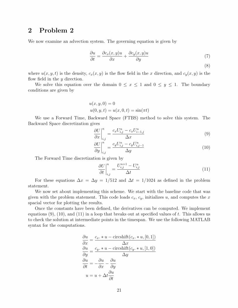
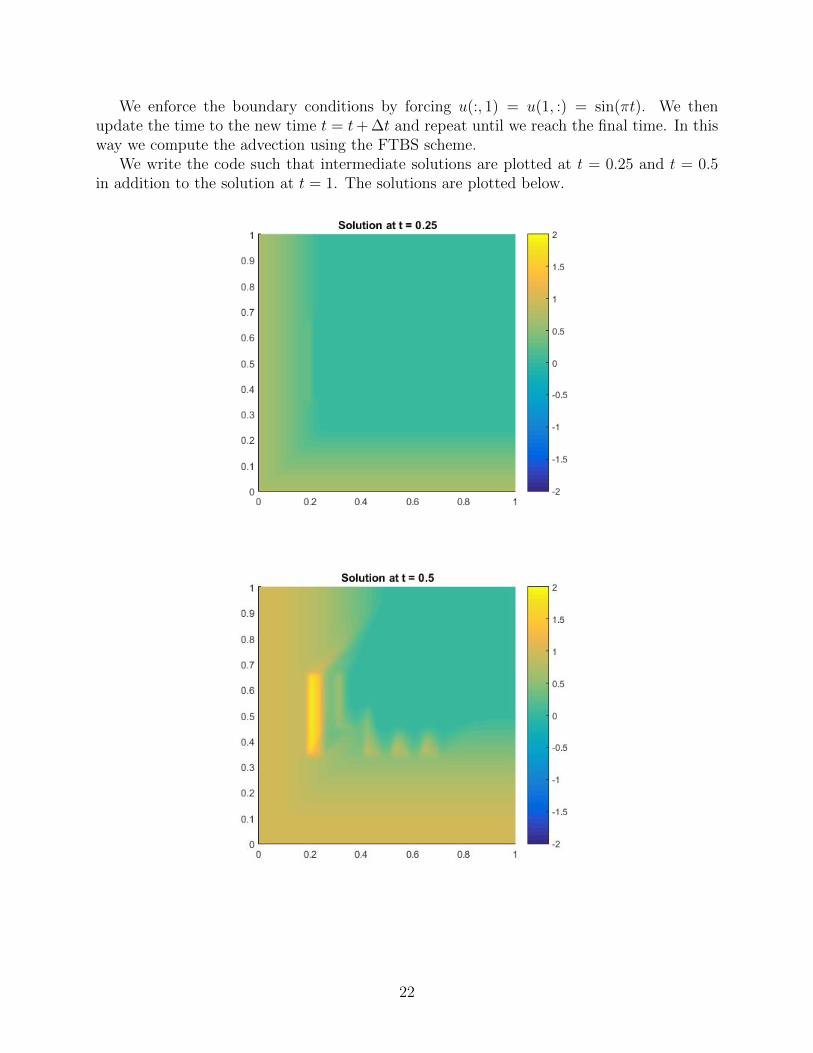
We write the code such that intermediate solutions are plotted at t = 0.25 and t = 0.5in addition to the solution at t = 1. The solutions are plotted below.

22

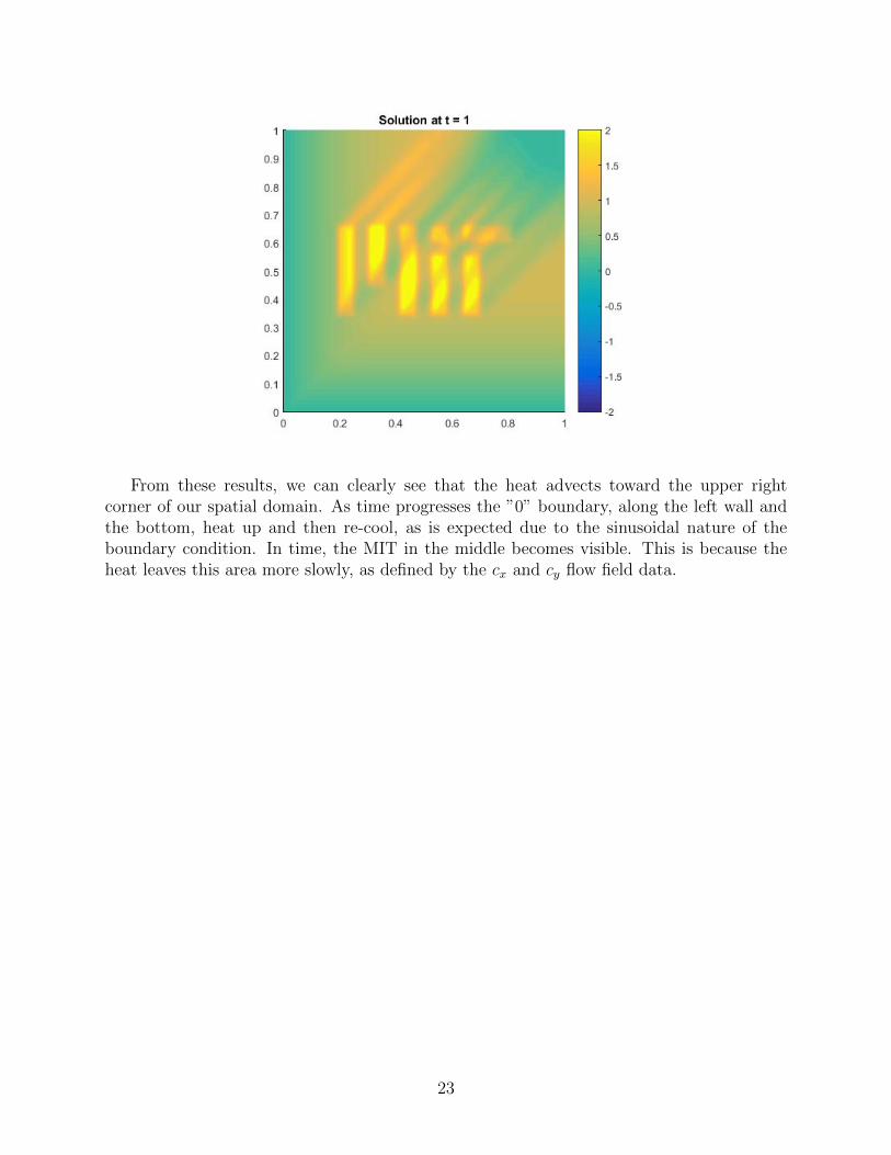
From these results, we can clearly see that the heat advects toward the upper rightcorner of our spatial domain. As time progresses the ”0” boundary, along the left wall andthe bottom, heat up and then re-cool, as is expected due to the sinusoidal nature of theboundary condition. In time, the MIT in the middle becomes visible. This is because theheat leaves this area more slowly, as defined by the cx and cy flow field data.

23

A AeroVibe.m

function [ sdot ] = AeroVibe( s )

%AeroVibe Compute derivatives for elastic wing

% compute derivatives of pitch and height for Aeroelastic wing model

% Global variable Q must be defined for this code to compile

% s = [a, a_dot, h, h_dot]

% sdot = [a_dot, a_dotdot, h_dot, h_dotdot]

global Q

Mhh = 1;

Mha = 0.625;

Maa = 1.25;

Mah = 0.25;

Dh = 0.1;

Da = 0.25;

Kh = 0.2;

Ka = 1.25;

kNL = 10;

a = s(1);

a_dot = s(2);

h = s(3);

h_dot = s(4);

L = Q*a;

M = -0.7*Q*a;

h_dotdot = (Mha/Maa*(Da*a_dot + Ka*(1+kNL*h^2)*a + M)...

- Dh*h_dot - Kh*h - L)/(Mhh - Mah*Mha/Maa);

a_dotdot = (Mah/Mhh*(Dh*h_dot + Kh*h + L)...

- Da*a_dot - Ka*(1+kNL*h^2)*a - M)/(Maa - Mah*Mha/Mhh);

sdot = [a_dot; a_dotdot; h_dot; h_dotdot];

24

B AeroVibeJacobian.m

function [ jac ] = AeroVibeJacobian( s )

%AEROVIBEJACOBIAN Computes Jacobian for an Aeroelastic wing system

% compute Jacobian matrix

%

% Global variable Q must be defined for this code to compile

% s = [a, a_dot, h, h_dot] --- Current state

%

% Jacobian = [ adot_a adot_adot adot_h adot_hdot;

% adotdot_a adotdot_adot adotdot_h adotdot_hdot;

% hdot_a hdot_adot hdot_h hdot_hdot;

% hdotdot_a hdotdot_adot hdotdot_h hdotdot_hdot];

global Q

Mhh = 1;

Mha = 0.625;

Maa = 1.25;

Mah = 0.25;

Dh = 0.1;

Da = 0.25;

Kh = 0.2;

Ka = 1.25;

kNL = 10;

a = s(1);

a_dot = s(2);

h = s(3);

h_dot = s(4);

adot_a = 0;

adot_adot = 1;

adot_h = 0;

adot_hdot = 0;

adotdot_a = (Mah/Mhh*Q - Ka*(1+kNL*h^2) + 0.7*Q)/(Maa - Mah*Mha/Mhh);

adotdot_adot = -Da/(Maa - Mah*Mha/Mhh);

adotdot_h = (Mah/Mhh*Kh - Ka*kNL*2*h*a)/(Maa - Mah*Mha/Mhh);

adotdot_hdot = (Mah/Mhh*Dh)/(Maa - Mah*Mha/Mhh);

hdot_a = 0;

hdot_adot = 0;

hdot_h = 0;

hdot_hdot = 1;

25

hdotdot_a = (Mha/Maa*(Ka*(1+kNL*h^2) - 0.7*Q) - Q)/(Mhh - Mah*Mha/Maa);

hdotdot_adot = (Mha/Maa*Da)/(Mhh - Mah*Mha/Maa);

hdotdot_h = (Mha/Maa*(Ka*kNL*2*h*a) - Kh)/(Mhh - Mah*Mha/Maa);

hdotdot_hdot = -Dh/(Mhh - Mah*Mha/Maa);

jac = [ adot_a adot_adot adot_h adot_hdot;

adotdot_a adotdot_adot adotdot_h adotdot_hdot;

hdot_a hdot_adot hdot_h hdot_hdot;

hdotdot_a hdotdot_adot hdotdot_h hdotdot_hdot];

end

26

C ForwardEuler.m

function [ t, x ] = ForwardEuler( funcName, x_0, tspan, dt )

%FORWARDEULER Compute a Forward Euler scheme

% [ t, x ] = ForwardEuler( funcName, x_0, tspan, dt )

% Takes in initial state and runs a Forward Euler scheme over tspan with

% dt size time steps. Outputs the solution [x] for all time [t]

%

% FORWARD EULER: v_n+1 = v_n + dt*f(v_n)

%--------------------------------------------------------------------------

% INPUTS

% funcName [string] - filename of function for computing the

% derivative of the state

% x_0 [vector] - input initial state

% tspan [T0 TFINAL] - define initial and final time

% dt - time step size

% define time span for calculation

t = tspan(1):dt:tspan(2);

% create function handle from filename

fh = str2func(funcName);

% initialize the output vector

x = zeros([length(x_0) length(t)]);

% input initial conditions

x(:,1) = x_0;

% run a Forward Euler scheme

for i = 1:length(t)-1

xdot = fh(x(:,i));

x(:,i+1) = x(:,i) + dt*xdot;

end

end

27

D Midpoint.m

function [ t, x ] = Midpoint( funcName, x_0, tspan, dt )

%MIDPOINT Compute a Midpoint scheme

% [ t, x ] = Midpoint( funcName, x_0, tspan, dt ) computes x(i+1) using a

% Midpoint scheme. Outputs the solution [x] for all time [t]

%

% MIDPOINT: v_n+1 = v_n-1 + 2*dt*f(v_n)

%--------------------------------------------------------------------------

% INPUTS

% funcName [string] - filename of function for computing the

% derivative of the state

% x_0 [vector] - input initial state

% tspan [T0 TFINAL] - define initial and final time

% dt - time step size

% compute time span

t = tspan(1):dt:tspan(2);

% create funtion handle for computing the state derivative

fh = str2func(funcName);

% initialize the solution matrix

x = zeros([length(x_0) length(t)]);

% set the initial conditions

x(:,1) = x_0;

% compute the second time step using Forward Euler

xdot = fh(x(:,1));

x(:,2) = x(:,1) + dt*xdot;

% run the Midpoint scheme

for i = 2:length(t)-1

xdot = fh(x(:,i));

x(:,i+1) = x(:,i-1) + 2*dt*xdot;

end

end

28

E BDF2.m

function [ t, x ] = BDF2( funcName, funcJac, x_0, tspan, dt, tol )

%BDF2 Solve stiff differential equations, 2nd Order, Backward step

% [ t, x ] = BDF2( funcName, funcJac, x_0, tspan, dt, tol )

% Solve an implicit system using a second order, backward differentiation

% scheme. Returns the solution matrix [x] for all time t in the time

% vector [t]

%

% BDF-2: v_n+1 = 4/3*v_n - 1/3*v_n-1 + 2/3*dt*f(v_n+1)

%--------------------------------------------------------------------------

% INPUTS

% funcName [string] - function that computes derivative of state

% funcJac [string] - function that computes Jacobian of state

% x_0 [vector] -

% tspan [T0 TFINAL] - define initial and final time

% dt - define time step size

% tol - define tolerance size. Used for calculating residual of

% system

% define time span

t = tspan(1):dt:tspan(2);

% create function handles for derivative and Jacobian functions

f = str2func(funcName);

fJac = str2func(funcJac);

% initialize solution matrix

x = zeros([length(x_0) length(t)]);

% input initial conditions

x(:,1) = x_0;

% compute the second time step in order to run the 2-step scheme

xdot = f(x(:,1));

x(:,2) = x(:,1) + dt*xdot;

% initialize the Identity matrix to the size of the system

I = eye(length(x(:,1)));

% run the BDF-2 scheme to compute x(:, i+1)

for i = 2:length(t)-1

% set initial guess to previous time step

w = x(:,i);

29

% compute initial residual

R = w - 4/3*x(:,i) + 1/3*x(:,i-1) - 2/3*dt*f(w);

% solve the implicit system until the desired tolerance is met

while max(abs(R)) > tol

% compute Jacobian

df = fJac(w);

% compute derivative of residual

dR = I - 2/3*dt*df;

% solve for dw

dw = -dR\R;

% update the guess of x(:, i+1)

w = w + dw;

% compute the new residual

R = w - 4/3*x(:,i) + 1/3*x(:,i-1) - 2/3*dt*f(w);

end

% save x(:,i+1)

x(:,i+1) = w;

end

end

30

F Part 2

% Alex Feldstein

% 16.90 Project 1 part 2: Advection

% Model an advection system with a given flow field which spells ’MIT’

clear all;

close all;

% load Cx and Cy from disk

Cx = load(’Cx.txt’);

Cy = load(’Cy.txt’);

% set the initial condition

u = zeros(size(Cx));

% set dt as given in the problem statement

dt = 1/1024;

% compute dx and dy

dx = 1/(length(Cx(:,1))-1);

dy = dx;

% compute the x and y spacial vectors

x = dx * [0:(size(Cx,1)-1)];

% initialize t

t = 0;

% compute the solution for the first time interval 0 <= t <= 0.25

while t <= 0.25

% implemtent a Bacward Space scheme

dudx = (Cx.*u - circshift(Cx.*u, [0,1]))/dx;

dudy = (Cy.*u - circshift(Cy.*u, [1,0]))/dy;

% use the advection equation

dudt = -dudx + -dudy;

% implement a forward time scheme

u = u + dt*dudt;

% enforce the boundary condition

u(1,:) = sin(t * pi);

u(:,1) = sin(t * pi);

31

% compute the new time

t = t + dt;

end

% plot the solution at t = 0.25

figure;

surf(x, x, u);

shading interp;

caxis([-2,2]);

view(2);

axis equal;

axis([0,1,0,1])

title(’Solution at t = 0.25’)

colorbar;

drawnow;

% run the solution over the second time interval 0.25 < t <= 0.5

while t <= 0.5

dudx = (Cx.*u - circshift(Cx.*u, [0,1]))/dx;

dudy = (Cy.*u - circshift(Cy.*u, [1,0]))/dy;

dudt = -dudx + -dudy;

u = u + dt*dudt;

% enforce the boundary condition

u(1,:) = sin(t * pi);

u(:,1) = sin(t * pi);

t = t + dt;

end

% plot the solution at t = 0.5

figure;

surf(x, x, u);

shading interp;

caxis([-2,2]);

view(2);

axis equal;

axis([0,1,0,1])

title(’Solution at t = 0.5’)

colorbar;

drawnow;

% run the solution over the third time interval 0.5 < t <= 1

32

while t <= 1

dudx = (Cx.*u - circshift(Cx.*u, [0,1]))/dx;

dudy = (Cy.*u - circshift(Cy.*u, [1,0]))/dy;

dudt = -dudx + -dudy;

u = u + dt*dudt;

% enforce the boundary condition

u(1,:) = sin(t * pi);

u(:,1) = sin(t * pi);

t = t + dt;

end

% plot the solution at t = 1

figure;

surf(x, x, u);

shading interp;

caxis([-2,2]);

view(2);

axis equal;

axis([0,1,0,1])

title(’Solution at t = 1’)

colorbar;

drawnow;

33

MIT OpenCourseWarehttp://ocw.mit.edu

16.90 Computational Methods in Aerospace EngineeringSpring 2014

For information about citing these materials or our Terms of Use, visit: http://ocw.mit.edu/terms.