11. Time series and dynamic linearmodels

Objective

To introduce the Bayesian approach to the modeling and forecasting of timeseries.

Recommended reading

• West, M. and Harrison, J. (1997). Bayesian forecasting and dynamicmodels, (2’nd ed.). Springer.

• Pole, A.,West, M. and Harrison, J. (1994). Applied Bayesian forecastingand time series analysis. Chapman and Hall.

• Bauwens, L., Lubrano, M. and Richard, J.F. (2000). Bayesian inference indynamic econometric models. Oxford University Press.

Bayesian Statistics

Dynamic linear models

West

The first Bayesian approach to forecasting stems from Harrison and Stevens(1976) and is based on the dynamic linear model. For a full discussion, seeWest and Harrison (1997).

Bayesian Statistics

The general DLM

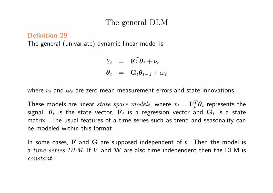
Definition 29The general (univariate) dynamic linear model is

Yt = FTt θt + νt

θt = Gtθt−1 + ωt

where νt and ωt are zero mean measurement errors and state innovations.

These models are linear state space models, where xt = FTt θt represents the

signal, θt is the state vector, Ft is a regression vector and Gt is a statematrix. The usual features of a time series such as trend and seasonality canbe modeled within this format.

In some cases, F and G are supposed independent of t. Then the model isa time series DLM. If V and W are also time independent then the DLM isconstant.

Bayesian Statistics

Examples

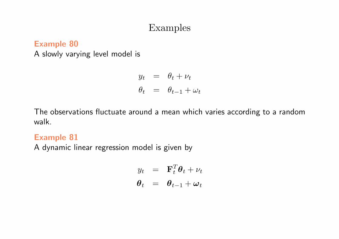
Example 80A slowly varying level model is

yt = θt + νt

θt = θt−1 + ωt

The observations fluctuate around a mean which varies according to a randomwalk.

Example 81A dynamic linear regression model is given by

yt = FTt θt + νt

θt = θt−1 + ωt

Bayesian Statistics

Bayesian analysis of DLM’s

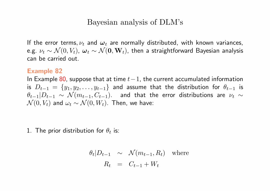
If the error terms, νt and ωt are normally distributed, with known variances,e.g. νt ∼ N (0, Vt), ωt ∼ N (0,Wt), then a straightforward Bayesian analysiscan be carried out.

Example 82In Example 80, suppose that at time t−1, the current accumulated informationis Dt−1 = {y1, y2, . . . , yt−1} and assume that the distribution for θt−1 isθt−1|Dt−1 ∼ N (mt−1, Ct−1). and that the error distributions are νt ∼N (0, Vt) and ωt ∼ N (0,Wt). Then, we have:

1. The prior distribution for θt is:

θt|Dt−1 ∼ N (mt−1, Rt) where

Rt = Ct−1 + Wt

Bayesian Statistics

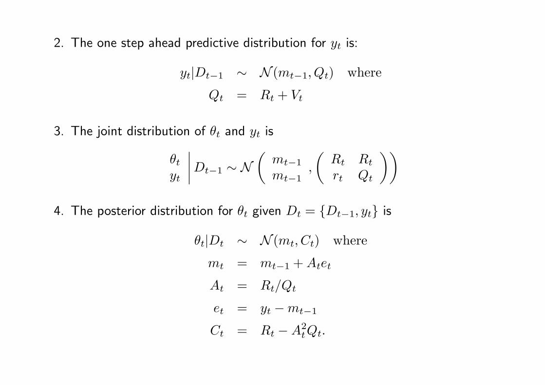
2. The one step ahead predictive distribution for yt is:

yt|Dt−1 ∼ N (mt−1, Qt) where

Qt = Rt + Vt

3. The joint distribution of θt and yt is

θt

yt

∣∣∣∣ Dt−1 ∼ N(

mt−1

mt−1,

(Rt Rt

rt Qt

))4. The posterior distribution for θt given Dt = {Dt−1, yt} is

θt|Dt ∼ N (mt, Ct) where

mt = mt−1 + Atet

At = Rt/Qt

et = yt −mt−1

Ct = Rt −A2tQt.

Bayesian Statistics

Proof and observations

Proof The first three steps of the proof are straightforward just by goingthrough the observation and system equations. The posterior distributionfollows from property iv) of the multivariate normal distribution as given inDefinition 22.

In the formula for the posterior mean, et is simply a prediction error term.This formula could also be rewritten as a weighted average in the usual wayfor normal models:

mt = (1−At)mt−1 + Atyt.

Bayesian Statistics

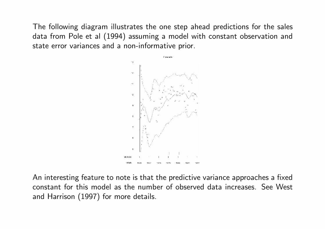
The following diagram illustrates the one step ahead predictions for the salesdata from Pole et al (1994) assuming a model with constant observation andstate error variances and a non-informative prior.

An interesting feature to note is that the predictive variance approaches a fixedconstant for this model as the number of observed data increases. See Westand Harrison (1997) for more details.

Bayesian Statistics

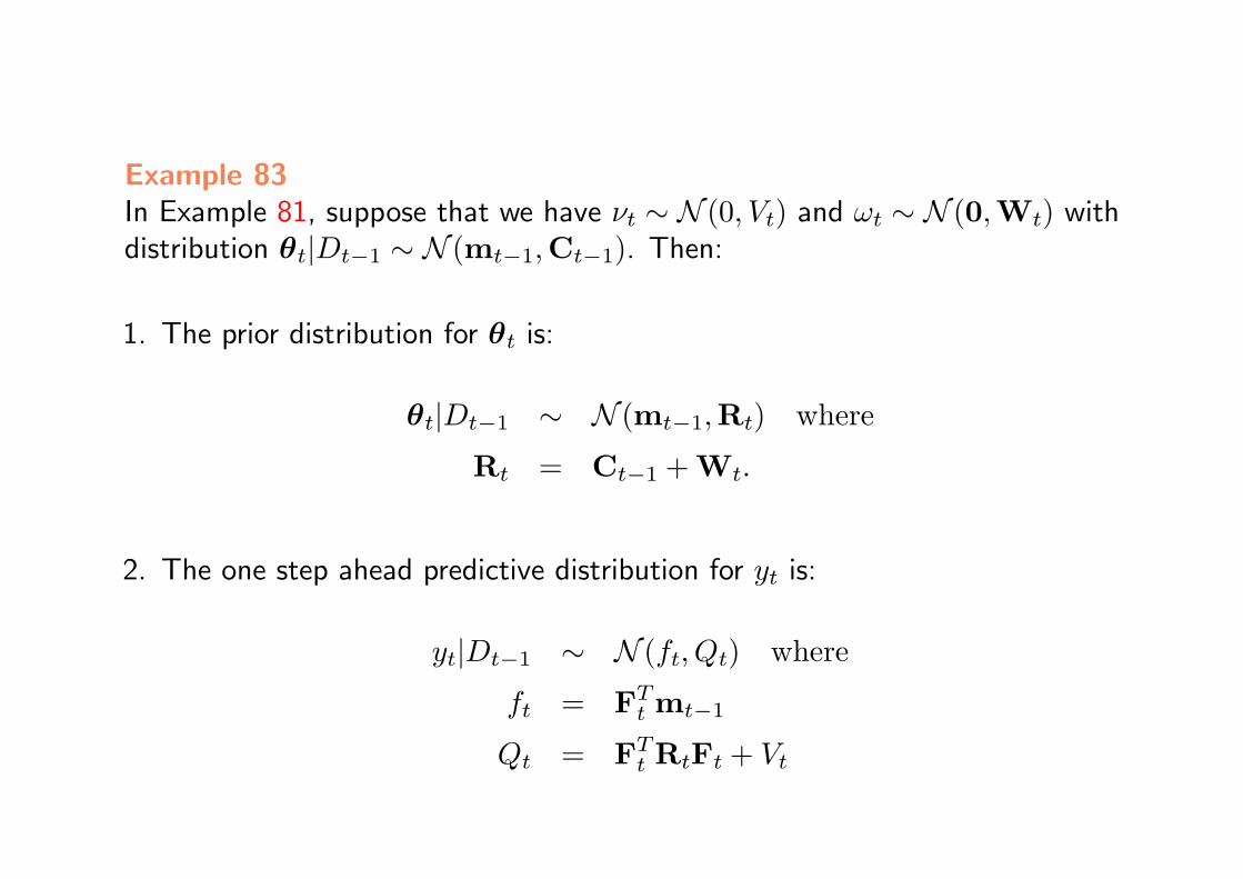
Example 83In Example 81, suppose that we have νt ∼ N (0, Vt) and ωt ∼ N (0,Wt) withdistribution θt|Dt−1 ∼ N (mt−1,Ct−1). Then:

1. The prior distribution for θt is:

θt|Dt−1 ∼ N (mt−1,Rt) where

Rt = Ct−1 + Wt.

2. The one step ahead predictive distribution for yt is:

yt|Dt−1 ∼ N (ft, Qt) where

ft = FTt mt−1

Qt = FTt RtFt + Vt

Bayesian Statistics

3. The joint distribution of θt and yt is

θt

yt

∣∣∣∣ Dt−1 ∼ N(

mt−1

ft,

(Rt FT

t Rt

RtFt Qt

))

4. The posterior distribution for θt given Dt = {Dt−1, yt} is

θt|Dt ∼ N (mt,Ct) where

mt = mt−1 + Atet

Ct = Rt −AtATt Qt

At = RtFtQ−1t

et = yt − ft.

Proof Exercise.

Bayesian Statistics

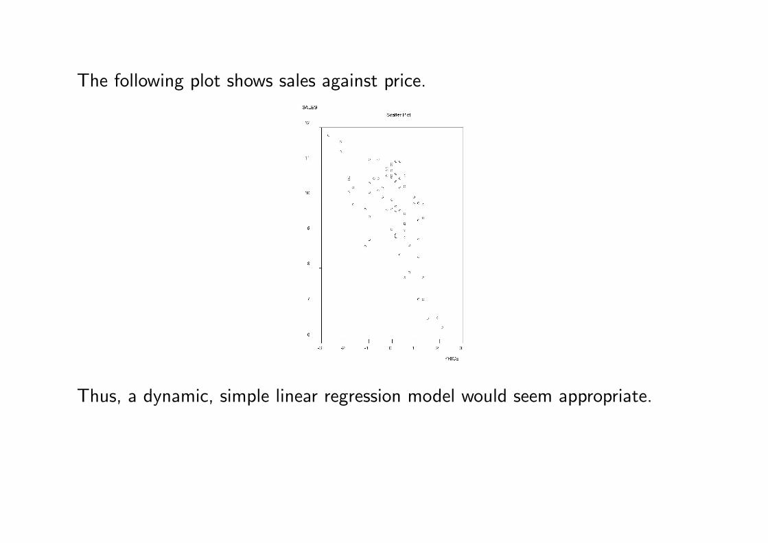
The following plot shows sales against price.

Thus, a dynamic, simple linear regression model would seem appropriate.

Bayesian Statistics

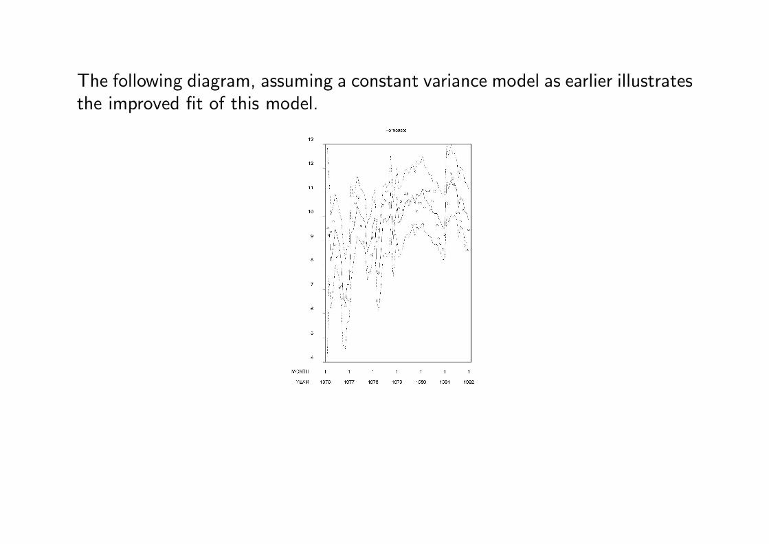
The following diagram, assuming a constant variance model as earlier illustratesthe improved fit of this model.

Bayesian Statistics

The general theorem for DLM’s

Theorem 43For the general, univariate DLM,

Yt = FTt θt + νt

θt = Gtθt−1 + ωt

where νt ∼ N (0, Vt) and ωt ∼ N (0,Wt), assuming the prior distributionθt−1|Dt−1 ∼ N (mt−1,Ct−1), we have

1. Prior distribution for θt:

θt|Dt−1 ∼ N (at,Rt) where

at = Gtmt−1

Rt = GtCt−1GTt + Wt

Bayesian Statistics

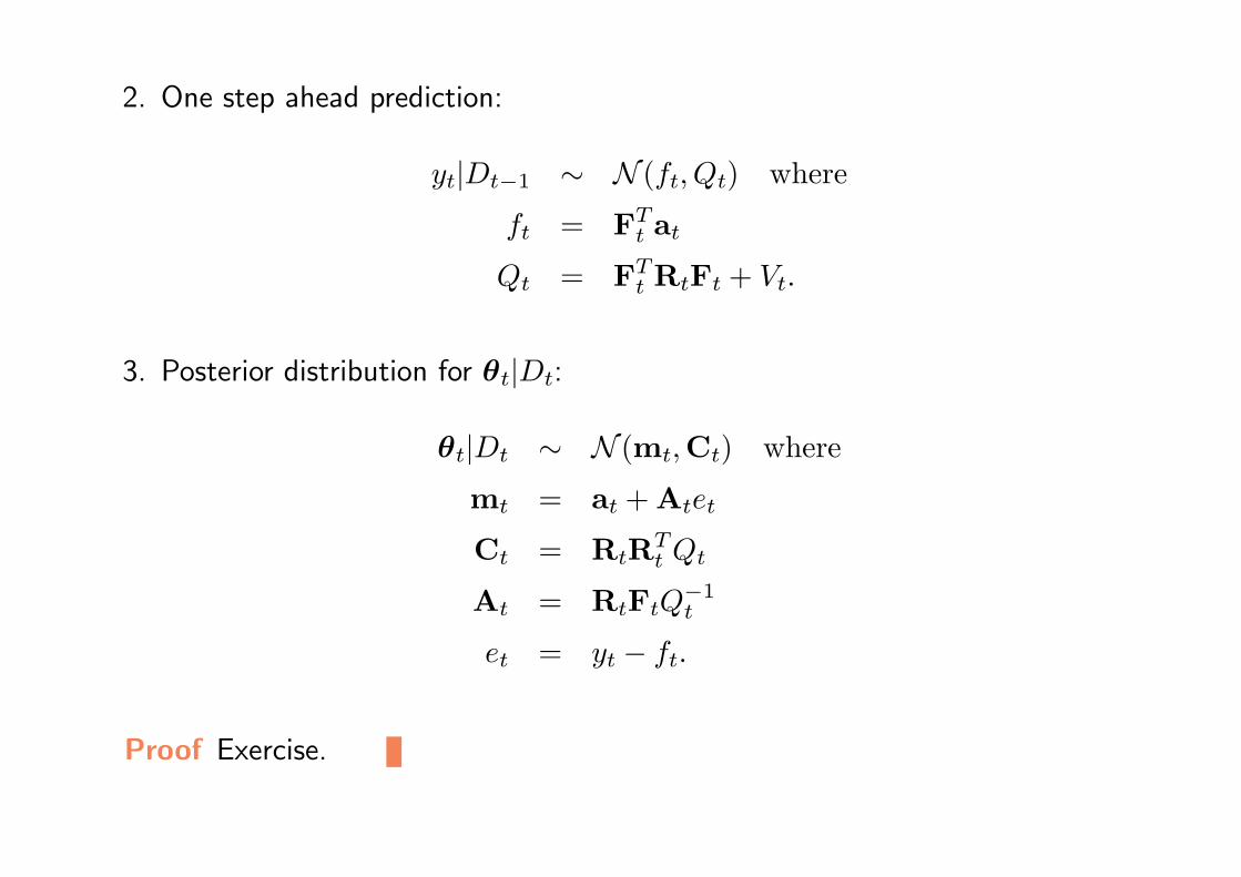
2. One step ahead prediction:

yt|Dt−1 ∼ N (ft, Qt) where

ft = FTt at

Qt = FTt RtFt + Vt.

3. Posterior distribution for θt|Dt:

θt|Dt ∼ N (mt,Ct) where

mt = at + Atet

Ct = RtRTt Qt

At = RtFtQ−1t

et = yt − ft.

Proof Exercise.

Bayesian Statistics

DLM’s and the Kalman filter

The updating equations in the general theorem are essentially those used inthe Kalman filter developed in Kalman (1960) and Kalman and Bucy (1961).For more details, see

http://en.wikipedia.org/wiki/Kalman_filter

Bayesian Statistics

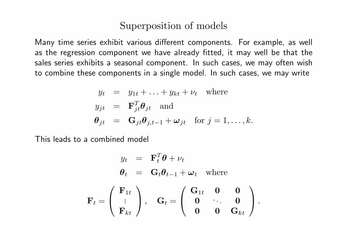
Superposition of models

Many time series exhibit various different components. For example, as wellas the regression component we have already fitted, it may well be that thesales series exhibits a seasonal component. In such cases, we may often wishto combine these components in a single model. In such cases, we may write

yt = y1t + . . . + ykt + νt where

yjt = FTjtθjt and

θjt = Gjtθj,t−1 + ωjt for j = 1, . . . , k.

This leads to a combined model

yt = FTt θ + νt

θt = Gtθt−1 + ωt where

Ft =

F1t...

Fkt

, Gt =

G1t 0 00 . . . 00 0 Gkt

.

Bayesian Statistics

Bayesian Statistics

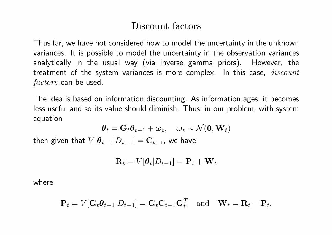
Discount factors

Thus far, we have not considered how to model the uncertainty in the unknownvariances. It is possible to model the uncertainty in the observation variancesanalytically in the usual way (via inverse gamma priors). However, thetreatment of the system variances is more complex. In this case, discountfactors can be used.

The idea is based on information discounting. As information ages, it becomesless useful and so its value should diminish. Thus, in our problem, with systemequation

θt = Gtθt−1 + ωt, ωt ∼ N (0,Wt)then given that V [θt−1|Dt−1] = Ct−1, we have

Rt = V [θt|Dt−1] = Pt + Wt

where

Pt = V [Gtθt−1|Dt−1] = GtCt−1GTt and Wt = Rt −Pt.

Bayesian Statistics

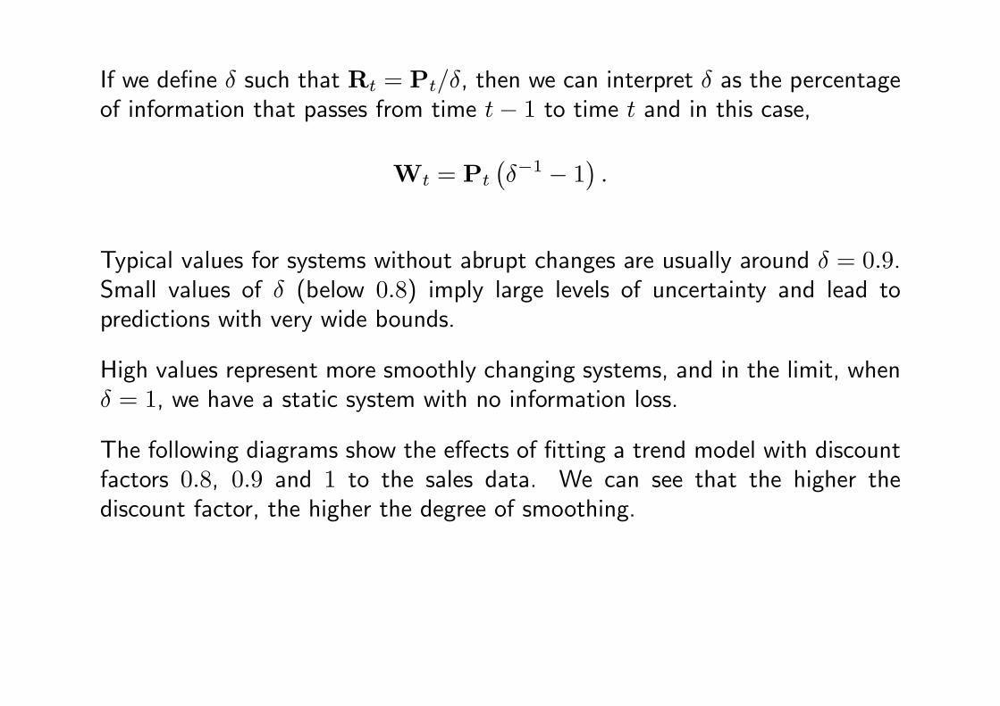
If we define δ such that Rt = Pt/δ, then we can interpret δ as the percentageof information that passes from time t− 1 to time t and in this case,

Wt = Pt

(δ−1 − 1

).

Typical values for systems without abrupt changes are usually around δ = 0.9.Small values of δ (below 0.8) imply large levels of uncertainty and lead topredictions with very wide bounds.

High values represent more smoothly changing systems, and in the limit, whenδ = 1, we have a static system with no information loss.

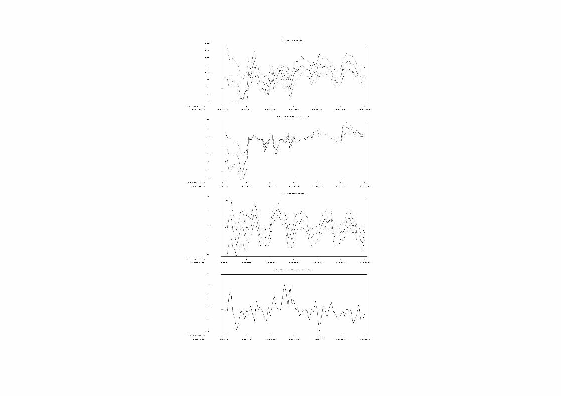
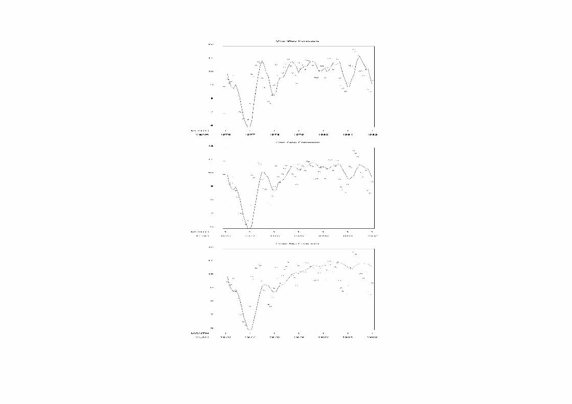
The following diagrams show the effects of fitting a trend model with discountfactors 0.8, 0.9 and 1 to the sales data. We can see that the higher thediscount factor, the higher the degree of smoothing.

Bayesian Statistics

Bayesian Statistics

The forward filtering backward sampling algorithm

This algorithm, developed in Carter and Kohn (1994) and Fruhwirth-Schnatter(1994) allows for the implementation of an MCMC approach to DLM’s.

The forward filtering step is the standard normal linear analysis to give p(θt|Dt)at each t, for t = 1, . . . , n.

The backward sampling step uses the Markov property and samples θ?n from

p(θn|Dn) and then, for t = 1, . . . , n − 1, samples θ?t from p(θt|Dt,θ

?t+1).

Thus, a sample from the posterior parameter structure is generated.

Bayesian Statistics

Example: the AR(p) model with time varying coefficients

Example 84The AR(p) model with time varying coefficients takes the form

yt = θ0t + θ1t + . . . + θptyt−p + νt

θit = θi,t−1 + ωit

where we shall assume that the error terms are independent normals:

νit ∼ N (0, V ) and ωit ∼ N (0, λiV ).

Then this model can be expressed in state space form by setting

θt = (θ0t, . . . , θpt)T

F = (1, yt−1, . . . , yt−p)T

G = Ip+1

W = V diag(λ)

Bayesian Statistics

Here diag(λ) represents a diagonal matrix with ii’th entry equal to λi, fori = 1, . . . , p + 1.

Now, given gamma priors for V and for λ−1i and a normal prior for θ0, then it

is clear that the relevant posterior distributions are all conditionally conjugate.

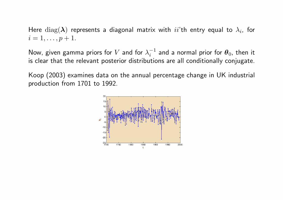
Koop (2003) examines data on the annual percentage change in UK industrialproduction from 1701 to 1992.

Bayesian Statistics

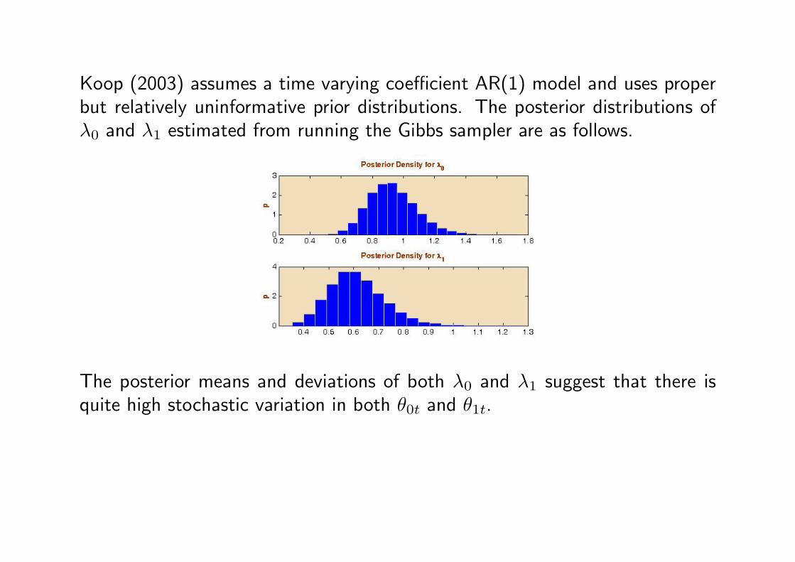
Koop (2003) assumes a time varying coefficient AR(1) model and uses properbut relatively uninformative prior distributions. The posterior distributions ofλ0 and λ1 estimated from running the Gibbs sampler are as follows.

The posterior means and deviations of both λ0 and λ1 suggest that there isquite high stochastic variation in both θ0t and θ1t.

Bayesian Statistics

Software for fitting DLM’s

Two general software packages are available.

• BATS. Pole et al (1994). This (somewhat out of date) package can be usedto perform basic analyses and is available from:

http://www.stat.duke.edu/~mw/bats.html

• dlm. Petris (2006). This is a recently produced R package for fittingDLM’s, including ARMA models etc. available from

http://cran.r-project.org/src/contrib/Descriptions/dlm.html

Bayesian Statistics

Other work in time series

• ARMA and ARIMA models. Marriot and Newbold (1998).

• Non linear and non normal state space models. Carlin et al (1992).

• Latent structure models. Aguilar et al (1998).

• Stochastic volatility models. Jacquier et al (1994).

• GARCH and other econometric models. Bauwens et al (2000).

• Wavelets. Nason and Sapatinas (2002).

Bayesian Statistics

References

Aguilar, O., Huerta, G., Prado, R. and West, M. (1998). Bayesian inference on latent

structure in time series. In Bayesian Statistics 6 eds. Bernardo et al. Oxford: University

Press.

Bauwens, L., Lubrano, M. and Richard, J.F. (2000). Bayesian inference in dynamiceconometric models. Oxford University Press.

Carlin, B.P., Poison, N.G. and Stoffer, D.S. (1992). A Monte Carlo approach to nonnormal

and nonlinear state space modeling. Journal of the American Statistical Association, 87,

493–500.

Carter, C.K. and Kohn, R. (1996). Markov chain Monte Carlo in conditionally Gaussian

state space models. Biometrika, 83, 589–601.

Fruhwirth-Schnatter, S. (1994). Data augmentation and dynamic linear models. Journalof Time Series Analysis, 15, 183–202.

Harrison, P.J. and Stevens, C.F. (1976). Bayesian forecasting (with discussion). Journalof the Royal Statistical Society Series B, 38, 205-247.

Jacquier, E., Polson, N.G. and Rossi, P.E. (1994). Bayesian Analysis of Stochastic Volatility

Models. Journal of Business & Economic Statistics, 12, 371–389.

Kalman, R.E. (1960). A new approach to linear filtering and prediction problems. Journalof Basic Engineering Series D, 82, 34-45.

Bayesian Statistics

Kalman, R.E. and Bucy, R.S. (1961). New Results in Linear Filtering and Prediction

Theory. Journal of Basic Engineering Series D, 83, 95-108.

Koop, G. (2003). Bayesian Econometrics. New York: Wiley.

Marriott, J. and Newbold, P. (1998). Bayesian Comparison of ARIMA and Stationary

ARMA Models. International Statistical Review, 66, 323–336.

Nason, G.P. and Sapatinas, T. (2002). Wavelet packet transfer function modelling of

nonstationary time series. Statistics and Computing, 12, 45–56.

Pole, A.,West, M. and Harrison, J. (1994). Applied Bayesian forecasting and time seriesanalysis. Chapman and Hall.

West, M. and Harrison, J. (1997). Bayesian forecasting and dynamic models, (2’nd ed.).

Springer.

Bayesian Statistics