General truncated linear statistics for the top

eigenvalues of random matrices

Aurelien Grabsch

Sorbonne Universite, CNRS, Laboratoire de Physique Theorique de la Matiere

Condensee (LPTMC), 4 Place Jussieu, 75005 Paris, France

Abstract. Invariant ensemble, which are characterised by the joint distribution of

eigenvalues P (λ1, . . . , λN ), play a central role in random matrix theory. We consider

the truncated linear statistics LK =∑Kn=1 f(λn) with 1 6 K 6 N , λ1 > λ2 > · · · > λN

and f a given function. This quantity has been studied recently in the case where the

function f is monotonous. Here, we consider the general case, where this function can

be non-monotonous. Motivated by the physics of cold atoms, we study the example

f(λ) = λ2 in the Gaussian ensembles of random matrix theory. Using the Coulomb

gas method, we obtain the distribution of the truncated linear statistics, in the limit

N → ∞ and K → ∞, with κ = K/N fixed. We show that the distribution presents

two essential singularities, which arise from two infinite order phase transitions for the

underlying Coulomb gas. We further argue that this mechanism is universal, as it

depends neither on the choice of the ensemble, nor on the function f .

arX

iv:2

111.

0900

4v1

[co

nd-m

at.s

tat-

mec

h] 1

7 N

ov 2

021

General truncated linear statistics for the top eigenvalues of random matrices 2

Contents

1 Introduction 2

1.1 Main results . . . . . . . . . . . . . . . . . . . . . . . . . . . . . . . . . . 5

1.2 Outline of the paper . . . . . . . . . . . . . . . . . . . . . . . . . . . . . 7

2 The Coulomb gas method for general truncated linear statistics 7

2.1 Saddle point equations and large deviation function . . . . . . . . . . . . 8

2.2 Reformulation and solution of the saddle-point equation . . . . . . . . . . 9

3 Application to a system of fermions 12

3.1 Optimal density without constraint . . . . . . . . . . . . . . . . . . . . . 13

3.2 Phase I: two disjoint supports . . . . . . . . . . . . . . . . . . . . . . . . 14

3.3 Phase II: a logarithmic singularity . . . . . . . . . . . . . . . . . . . . . . 15

3.4 Two infinite order phase transitions . . . . . . . . . . . . . . . . . . . . . 17

3.5 Distribution of the potential energy of the K rightmost fermions . . . . . 18

4 Universality 21

5 Conclusion 22

Appendix A A few useful integrals 23

Appendix B Infinite order phase transitions 23

1. Introduction

Random matrix theory has first been introduced in physics by Wigner and Dyson

in the 1950s to model the atomic nucleus [1]. It has now been successfully applied

in various domains of physics, such as electronic quantum transport [2–14], quantum

information [15–20], statistical physics of fluctuating interfaces [21, 22] or cold atoms

[23,24].

Invariant ensembles play a prominent role in random matrix theory. They

correspond to distributions of matrices which are invariant under changes of basis.

Consequently, the eigenvalues and eigenvectors are statistically independent, and one

can focus on the eigenvalues only. In the most famous invariant ensembles, the joint

distribution of the eigenvalues takes the form [25–27]

P (λ1, . . . , λN) ∝∏i<j

|λi − λj|βN∏n=1

e−βN2V (λn) , (1)

General truncated linear statistics for the top eigenvalues of random matrices 3

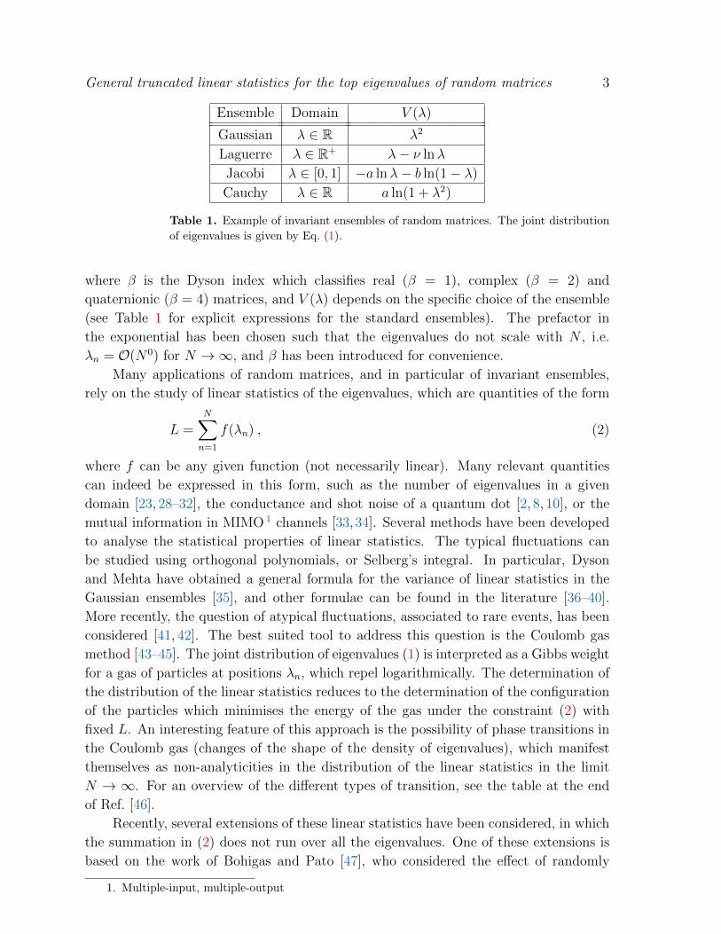
Ensemble Domain V (λ)

Gaussian λ ∈ R λ2

Laguerre λ ∈ R+ λ− ν lnλ

Jacobi λ ∈ [0, 1] −a lnλ− b ln(1− λ)

Cauchy λ ∈ R a ln(1 + λ2)

Table 1. Example of invariant ensembles of random matrices. The joint distribution

of eigenvalues is given by Eq. (1).

where β is the Dyson index which classifies real (β = 1), complex (β = 2) and

quaternionic (β = 4) matrices, and V (λ) depends on the specific choice of the ensemble

(see Table 1 for explicit expressions for the standard ensembles). The prefactor in

the exponential has been chosen such that the eigenvalues do not scale with N , i.e.

λn = O(N0) for N →∞, and β has been introduced for convenience.

Many applications of random matrices, and in particular of invariant ensembles,

rely on the study of linear statistics of the eigenvalues, which are quantities of the form

L =N∑n=1

f(λn) , (2)

where f can be any given function (not necessarily linear). Many relevant quantities

can indeed be expressed in this form, such as the number of eigenvalues in a given

domain [23, 28–32], the conductance and shot noise of a quantum dot [2, 8, 10], or the

mutual information in MIMO 1 channels [33,34]. Several methods have been developed

to analyse the statistical properties of linear statistics. The typical fluctuations can

be studied using orthogonal polynomials, or Selberg’s integral. In particular, Dyson

and Mehta have obtained a general formula for the variance of linear statistics in the

Gaussian ensembles [35], and other formulae can be found in the literature [36–40].

More recently, the question of atypical fluctuations, associated to rare events, has been

considered [41, 42]. The best suited tool to address this question is the Coulomb gas

method [43–45]. The joint distribution of eigenvalues (1) is interpreted as a Gibbs weight

for a gas of particles at positions λn, which repel logarithmically. The determination of

the distribution of the linear statistics reduces to the determination of the configuration

of the particles which minimises the energy of the gas under the constraint (2) with

fixed L. An interesting feature of this approach is the possibility of phase transitions in

the Coulomb gas (changes of the shape of the density of eigenvalues), which manifest

themselves as non-analyticities in the distribution of the linear statistics in the limit

N → ∞. For an overview of the different types of transition, see the table at the end

of Ref. [46].

Recently, several extensions of these linear statistics have been considered, in which

the summation in (2) does not run over all the eigenvalues. One of these extensions is

based on the work of Bohigas and Pato [47], who considered the effect of randomly

1. Multiple-input, multiple-output

General truncated linear statistics for the top eigenvalues of random matrices 4

removing each eigenvalue with a given probability. This situation is described by the

so-called thinned ensembles, which have been the focus of several works over the last

years [48–50], studying in particular linear statistics (see also [51] for a related problem).

Alternatively, one can choose deterministically a subset of the eigenvalues 2 {λn},and compute the associated linear statistics. This situation has been first considered

in [46], where only a given number K 6 N of the largest eigenvalues were selected,

leading to consider the truncated linear statistics

LK =K∑n=1

f(λn) , λ1 > λ2 > · · · > λN . (3)

This situation occurs naturally in various contexts, for instance in principal component

analysis, where one focuses on a given number of the largest eigenvalues since they

contain the most relevant information [30, 52]. The truncated linear statistics (3)

interpolates between the usual linear statistics (2) for K = N , and the largest eigenvalue

only for K = 1, which is also a widely studied quantity [41, 42, 53–58]. The statistical

properties of such truncated linear statistics have been studied in Ref. [46] in the bulk

regime N → ∞ and K → ∞ with κ = K/N fixed, using the Coulomb gas method.

It was shown that the distribution of LK displays a singular behaviour at its typical

value, which originates from an infinite order phase transition in the underlying Coulomb

gas. This behaviour is universal, meaning that it neither depends on the choice of the

ensemble, nor on the choice of the function f , provided that it is monotonous. This

problem has also been considered in the edge regime N � K � 1, but again for a class

of monotonous functions [59]. Finally, truncated linear statistics have been studied for

the one dimensional plasma in Ref. [60], which is also a one dimensional gas of particles,

but with linear repulsion, and again for a monotonous function f .

The aim of this paper is to consider the general case where the function f can

be non-monotonous. This extension is crucial to study various important observables,

such as the entanglement entropy which corresponds to f(λ) = −λ lnλ. Our goal is to

determine the distribution of the rescaled truncated linear statistics (3)

PN,κ

(s =

LKN

)= N !× (4)∫

dλ1

∫ λ1

dλ2 · · ·∫ λN−1

dλN P (λ1, . . . , λN) δ

(s− 1

N

K∑n=1

f(λn)

)in the bulk regime N → ∞ and K → ∞ with κ = K/N fixed. Although we will

argue that our results are general, we will mostly focus on a specific example in order

to make the analysis more concrete. We will consider the simplest non-monotonous

function f(λ) = λ2, and work in the Gaussian ensembles (see Table 1). Besides being

2. A well-known duality between ensembles of random matrices is obtained by selecting a given

subset of eigenvalue. More precisely, the set of every second eigenvalues {λ2n}n=1,...,N of a matrix of

size (2N +1)× (2N +1) in the Gaussian Orthogonal Ensemble (β = 1) is distributed as the eigenvalues

of a N ×N matrix from the Gaussian Symplectic Ensemble (β = 4). Similar duality relations exist for

other ensembles of random matrices [26].

General truncated linear statistics for the top eigenvalues of random matrices 5

the most elementary example, this situation is also motivated by the physics of cold

atoms: the eigenvalues {λn} in the Gaussian ensemble with β = 2 can be interpreted

as the positions of N spinless fermions placed in a one-dimensional harmonic trap at

zero temperature. The corresponding truncated linear statistics (3) is then the potential

energy carried by the K rightmost fermions.

1.1. Main results

In the limit N → ∞, with κ = KN

fixed, the distribution of the truncated linear

statistics (3) with f(λ) = λ2 in the Gaussian ensembles (V (λ) = λ2) takes the form 3

PN,κ

(s =

LKN

)∼

N→∞exp

[−βN

2

2Φκ(s)

], (5)

where we have introduced the large deviation function Φκ, which has the following

behaviours:

Φκ(s) '

−κ2

2ln s for s→ 0 ,

(s− s0(κ))2

2F (c0(κ))for s→ s0(κ) ,

s− κ(2− κ)

2ln s for s→∞ ,

(6)

where s0(κ) is the typical value of the truncated linear statistics s, given by Eq. (47)

below, in terms of c0(κ) (48). The function F (c0) controls the variance of s, and is given

explicitly by (70). The function F , and thus the variance of s, displays a surprising

non-monotonous behaviour as a function of the fraction κ, as illustrated in Fig. 3 below.

This specific form of the distribution arises from a universal mechanism for the

underlying Coulomb gas. Indeed, in the limit N →∞, the distribution of the truncated

linear statistics is dominated by one optimal configuration of the eigenvalues (or charges

of the Coulomb gas). This optimal configuration is determined by the two parameters:

the fraction κ = K/N of eigenvalues under consideration, and s which controls the

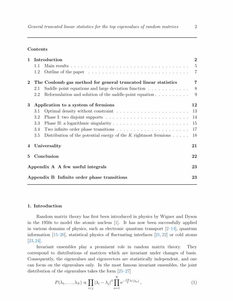
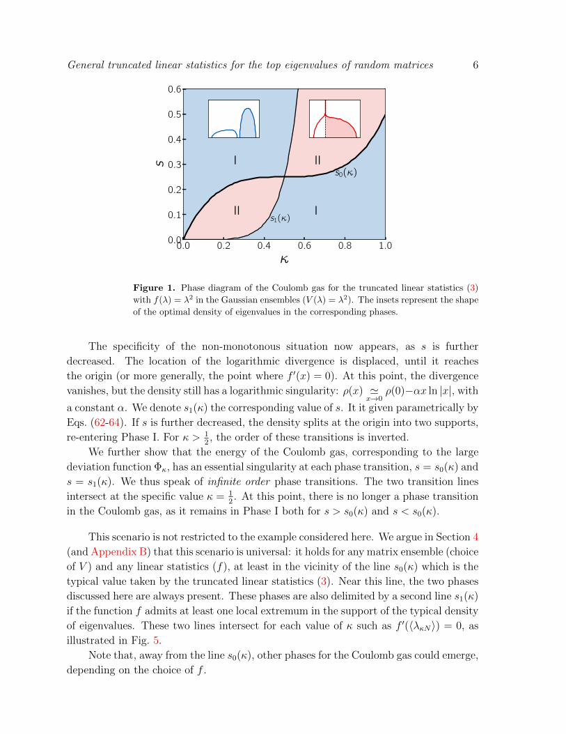
constraint in (4). The corresponding phase diagram is shown in Fig. 1.

For a fixed value of κ, the parameter s drives two consecutive phase transitions for

the Coulomb gas, corresponding to a change in the optimal configuration of eigenvalues

which dominates (4). The first phase (Phase I) corresponds to an optimal density of

eigenvalues supported on two disjoint supports. For instance, for κ < 12, it corresponds

to the region s > s0(κ). As s decreases, the gap between the two supports reduces,

until it completely closes when s = s0(κ). As s is further decreased, entering Phase II, a

logarithmic divergence emerges at the point where the two interval have merged. Up to

now, this scenario is identical to the one described in Ref. [46] in the case of monotonous

functions f .

3. Throughout the paper, the notation PN,κ(s) ∼N→∞

exp[−βN2

2 Φκ(s)] must be understood as

limN→∞2

βN2 lnPN,κ(s) = −Φκ(s).

General truncated linear statistics for the top eigenvalues of random matrices 6

0.0 0.2 0.4 0.6 0.8 1.0

κ

0.0

0.1

0.2

0.3

0.4

0.5

0.6

s

I

I II

II

s0(κ)

s1(κ)

Figure 1. Phase diagram of the Coulomb gas for the truncated linear statistics (3)

with f(λ) = λ2 in the Gaussian ensembles (V (λ) = λ2). The insets represent the shape

of the optimal density of eigenvalues in the corresponding phases.

The specificity of the non-monotonous situation now appears, as s is further

decreased. The location of the logarithmic divergence is displaced, until it reaches

the origin (or more generally, the point where f ′(x) = 0). At this point, the divergence

vanishes, but the density still has a logarithmic singularity: ρ(x) 'x→0

ρ(0)−αx ln |x|, with

a constant α. We denote s1(κ) the corresponding value of s. It it given parametrically by

Eqs. (62-64). If s is further decreased, the density splits at the origin into two supports,

re-entering Phase I. For κ > 12, the order of these transitions is inverted.

We further show that the energy of the Coulomb gas, corresponding to the large

deviation function Φκ, has an essential singularity at each phase transition, s = s0(κ) and

s = s1(κ). We thus speak of infinite order phase transitions. The two transition lines

intersect at the specific value κ = 12. At this point, there is no longer a phase transition

in the Coulomb gas, as it remains in Phase I both for s > s0(κ) and s < s0(κ).

This scenario is not restricted to the example considered here. We argue in Section 4

(and Appendix B) that this scenario is universal: it holds for any matrix ensemble (choice

of V ) and any linear statistics (f), at least in the vicinity of the line s0(κ) which is the

typical value taken by the truncated linear statistics (3). Near this line, the two phases

discussed here are always present. These phases are also delimited by a second line s1(κ)

if the function f admits at least one local extremum in the support of the typical density

of eigenvalues. These two lines intersect for each value of κ such as f ′(〈λκN〉) = 0, as

illustrated in Fig. 5.

Note that, away from the line s0(κ), other phases for the Coulomb gas could emerge,

depending on the choice of f .

General truncated linear statistics for the top eigenvalues of random matrices 7

1.2. Outline of the paper

The paper is organised as follows. In Section 2 we introduce the general formalism

of the Coulomb gas, applied to the study of truncated linear statistics. In Section 3 we

analyse in details an application of this formalism to a specific example of truncated

linear statistics, motivated by the study of a system of cold atoms. In Section 4 we

argue that the main features observed on this example are actually universal, as they

neither depend on the choice of the matrix ensemble, nor on the choice of truncated

linear statistics under consideration.

2. The Coulomb gas method for general truncated linear statistics

The idea of the Coulomb gas method is to rewrite the joint distribution (1) as a

Gibbs weight

P ({λn}) ∝ e−βN2

2Egas({λn}) , Egas({λn}) =

1

N

N∑n=1

V (λn)− 1

N2

∑i 6=j

ln |λi − λj| . (7)

The energy Egas describes a one dimensional gas of particles at positions {λn}, trapped in

a confining potential V (λ) and submitted to repulsive logarithmic interactions between

each other. We have placed a factor β in the exponential in (1) so that this energy

does not depend on β. In the limit N →∞, we expect that the typical distribution of

eigenvalues finds a balance between the interaction and the confinement energy. This

is achieved if λn = O(N0), which also implies that Egas({λn}) = O(N0). This is the

reason why we placed a factor N in the definition (1): it ensures that we manipulate

quantities which do not scale with N . We can then introduce the empirical density

ρ(x) =1

N

N∑n=1

δ(x− λn) , (8)

which leads us to rewrite the measure (1) as (we neglect the subleading entropic

contributions, which are of order O(N−1) [56, 61])

P (λ1, . . . , λN) dλ1 · · · dλN → e−βN2

2E [ρ] Dρ , (9)

where the energy E [ρ] is the continuous version of (7),

E [ρ] = −∫ρ(x)ρ(y) ln |x− y| dxdy +

∫ρ(x)V (x)dx . (10)

Finally, we rescale the truncated linear statistics (3) as

s =LKN

=

∫c

ρ(x)f(x)dx , (11)

where c = λK is a lower bound ensuring that the summation runs only on the K largest

eigenvalues. It can be determined as∫c

ρ(x)dx =K

N= κ . (12)

General truncated linear statistics for the top eigenvalues of random matrices 8

Our aim is to compute the distribution of the rescaled truncated linear statistics s,

which can be expressed in terms of integrals over the density:

PN,κ(s) = (13)∫dc

∫Dρ e−

βN2

2E [ρ] δ

(∫c

ρ(x)dx− κ)δ

(∫ρ(x)dx− 1

)δ

(∫c

f(x)ρ(x)dx− s)

∫dc

∫Dρ e−

βN2

2E [ρ] δ

(∫c

ρ(x)dx− κ)δ

(∫ρ(x)dx− 1

)2.1. Saddle point equations and large deviation function

When N →∞, the integrals in (13) are dominated by the minimum of the energy

E [ρ] under the constraints imposed by the Dirac δ-functions. These constraints can be

enforced by introducing three Lagrange multipliers µ(1)0 , µ

(2)0 , µ1. We thus consider

F [ρ;µ0, µ0, µ1] = E [ρ] + µ(1)0

(∫ c

ρ(x)dx− (1− κ)

)+ µ

(2)0

(∫c

ρ(x)dx− κ)

+ µ1

(∫c

f(x)ρ(x)dx− s). (14)

Let us first focus on the numerator in Eq. (13), and denote ρ?(x;κ, s) the density that

dominates these integrals. It can be obtained in two steps. First, we find the density

ρ(x;µ(1)0 , µ

(2)0 , µ1) solution of

δF

δρ(x)

∣∣∣∣ρ

= 0 , (15)

which yields explicitly the integral equation

2

∫ρ(y;µ

(1)0 , µ

(2)0 , µ1) ln |x− y| dy = V (x) +

{µ

(1)0 for x < c

µ(2)0 + µ1f(x) for x > c

(16)

which can be understood as the energy balance for the particle at point x between the

confinement and the logarithmic repulsion. The Lagrange multipliers µ(1)0 and µ

(2)0 can

be interpreted as chemical potentials fixing the fraction of particles respectively below

and above c. The effect of the constraint on s is to add an additional external potential,

proportional to µ1, which acts only on the K rightmost eigenvalues.

Then, we determine the values µ(1)?0 (κ, s), µ

(2)?0 (κ, s), µ?1(κ, s) of the Lagrange

multipliers in terms of the parameters κ and s by imposing the constraints:∫c

ρ(x;µ(1)?0 , µ

(2)?0 , µ?1)dx = κ ,

∫ c

ρ(x;µ(1)?0 , µ

(2)?0 , µ?1)dx = 1− κ (17)∫

c

f(x)ρ(x;µ(1)?0 , µ

(2)?0 , µ?1)dx = s . (18)

Finally, the density which dominates the integrals in the numerator of (13) is given by

ρ?(x;κ, s) = ρ(x;µ(1)?0 (κ, s), µ

(2)?0 (κ, s), µ?1(κ, s)) . (19)

For the denominator, we proceed similarly, but without the constraint on s. The

solution can be deduced from the one obtained above by setting µ1 = 0. Explicitly,

General truncated linear statistics for the top eigenvalues of random matrices 9

from the solution (19), it can be obtained by finding the value s0(κ) which verifies

µ1(κ, s0(κ)) = 0. We then deduce the density which dominates the denominator of (13)

as

ρ0(x) = ρ?(x;κ, s0(κ)) . (20)

Having obtained the densities of eigenvalues ρ?(x;κ, s) and ρ0(x) which dominate

respectively the numerator and the denominator of (13), we can evaluate the integrals

with a saddle point estimate, which yields

PN,κ(s) ∼N→∞

exp

{−βN

2

2Φκ(s)

}, (21)

where we have introduced the large deviation function

Φκ(s) = E [ρ?(x;κ, s)]− E [ρ0(x)] . (22)

This is the difference of energy between the two optimal configurations of eigenvalues

dominating the numerator and the denominator of (13), respectively. These energies

can be computed from the exact expressions of the densities using Eq. (10), but this

is in general a difficult task. However, an important simplification was introduced in

Ref. [13], based on the “thermodynamic” identity

dE [ρ?(x;κ, s)]

ds= −µ?1(κ, s) . (23)

See Refs. [62,63] for a more detailed discussion of this relation. It can be used to obtain

the large deviation function via a simple integration of the Lagrange multiplier µ?1(κ, s)

(which needs to be computed anyway to determine ρ?(x;κ, s)):

Φκ(s) =

∫ s0(κ)

s

µ?1(κ, t) dt . (24)

We will make extensive use of this relation to study of the distribution PN,κ(s).

To avoid cumbersome notations, the dependence of the density on the parameters

κ and s will be implicit from now on. We will also not distinguish the densities

ρ(x;µ(1)0 , µ

(2)0 , µ1) and ρ?(x;κ, s); both will be denoted ρ?(x) in the following.

Now that we have laid out the procedure to obtain the distribution PN,κ(s), the

main remaining task is to find the solution of the saddle-point equation (16).

2.2. Reformulation and solution of the saddle-point equation

In order to solve the saddle-point equation (16), it is convenient to take its

derivative:

2−∫

ρ?(y)

x− ydy = V ′(x) +

{0 for x < c

µ1f′(x) for x > c

(25)

where −∫

denotes a Cauchy principal value integral. This equation can be interpreted

as the force balance on the eigenvalue located at position x. The constraint on s then

acts as an additional force −µ1f′(x) acting on the K rightmost eigenvalues (the sign

General truncated linear statistics for the top eigenvalues of random matrices 10

comes from the fact that the force is the opposite of the derivative of the potential). It

is convenient to split the density ρ? into two densities: ρR describing the K rightmost

eigenvalues under consideration, and ρL for the others (see Figure 2),

ρR(x) =1

N

K∑n=1

δ(x− λn) , ρL(x) =1

N

N∑n=K+1

δ(x− λn) . (26)

Due to the confining potential, the eigenvalues remain in a bounded region in space,

hence the densities ρL and ρR have compact supports. Let us denote [a, b] the support

of ρL, and [c, d] the support of ρR, where c is the boundary introduced previously in

Eqs. (11,12), as shown in Figure 2. Note that it is possible that the two supports merge,

so that b = c, as shown in Fig. 2 (right). We rewrite Eq. (25) in terms of these densities

as

2

∫ b

a

ρL(y)

x− ydy + 2−

∫ d

c

ρR(y)

x− ydy = V ′(x) + µ1f

′(x) for x ∈ [c, d] (27)

2−∫ b

a

ρL(y)

x− ydy + 2

∫ d

c

ρR(y)

x− ydy = V ′(x) for x ∈ [a, b] . (28)

In these two equations, the principal value is only required when x belongs to the domain

of the integral. Such principal value integral equations can be solved using a theorem due

to Tricomi [64], which gives an explicit expression for the inversion of Cauchy singular

equations of the form

−∫

ρ(y)

x− ydy = g(x) , (29)

under the assumption that the solution has one single support [a, b] [64]:

ρ(x) =1

π√

(x− a)(b− x)

{A+−

∫ b

a

dt

π

√(t− a)(b− t)t− x

g(t)

}, (30)

where A =∫ baρ(x)dx is a constant. In our case, solving the coupled equations (27,28)

requires to perform a double iteration of this theorem, in order to first determine ρL and

then ρR, as in Refs. [29,46]. This procedure is rather cumbersome, but it yields explicit

expressions for the densities ρL and ρR.

For the case of the Laguerre ensembles of random matrix theory (which corresponds

to a specific V (x) given in Table 1) and for monotonous functions f , the derivation is

performed in the Appendix of Ref. [46]. Here we adapt this procedure for the general

situation. The first step is to use Tricomi’s theorem to solve (28) for ρL, treating ρR as a

known function. Assuming that ρL has a compact support [a, b], we directly apply (30),

with

g(t) =1

2V ′(t)−

∫ d

c

ρR(y)

t− ydy (31)

and A =∫ baρL = 1 − κ from the constraint (17). After permuting the integrals, and

using (A.1), we obtain

ρL(x) =1

π√

(x− a)(b− x)

{1 +

1

2−∫ b

a

dt

πV ′(t)

√(t− a)(b− t)t− x

General truncated linear statistics for the top eigenvalues of random matrices 11

−∫ d

c

dy ρR(y)

√(y − a)(y − b)

y − x

}. (32)

Using now this expression in the second saddle-point equation (27), combined with the

integral (A.2), we obtain an equation for ρR only, valid for x ∈ [c, d]:

−∫ d

c

dyρR(y)

x− y√

(y − a)(y − b) =1

2

√(x− a)(x− b)(V ′(x) + µ1f

′(x))

− 1 +1

2

∫ b

a

dt

π

V ′(t)

x− t√

(t− a)(b− t) . (33)

We can solve this second equation using again Tricomi’s theorem (30), assuming that

ρR has a compact support [c, d]. This yields

ρR(x) =1

π√

(x− a)(x− b)(x− c)(d− x)

{− 1

2

∫ b

a

dt

π

V ′(t)

t− x√

(t− a)(b− t)(c− t)(d− t)

+C + x+1

2−∫ d

c

dt

π

V ′(t) + µ1f′(t)

t− x√

(t− a)(t− b)(t− c)(d− t)}, (34)

where C is a constant that combines the integration constant from Tricomi’s theorem

and other terms arising from the evaluation of the integrals. The expression for ρL can

be obtained by plugging this result into (32),

ρL(x) =−1

π√

(x− a)(b− x)(c− x)(d− x)

{− 1

2−∫ b

a

dt

π

V ′(t)

t− x√

(t− a)(b− t)(c− t)(d− t)

+C + x+1

2

∫ d

c

dt

π

V ′(t) + µ1f′(t)

t− x√

(t− a)(t− b)(t− c)(d− t)}. (35)

The constant C can then be determined in the following way. Since c corresponds

to the value λK of the Kth eigenvalue, it can freely fluctuate. Therefore, we do not

expect that the density of eigenvalues diverges as ρx(x) ∼ (x − c)−1/2 for x → c, as

this type of behaviour typically occurs near a hard edge, which is a hard constraint

on the eigenvalues (such as λn > 0). Therefore, the bracket in (34) must vanish for

x = c. This determines the value of the constant C, which we can now use to simplify

the expressions (34,35). We can actually express the total density ρ? = ρL ∪ ρR in a

compact form:

ρ?(x) =1

2π

√c− x

(x− a)(b− x)(d− x)

{2 +−

∫ b

a

dt

π

V ′(t)

t− x

√(t− a)(b− t)(d− t)

c− t

+−∫ d

c

dt

π

V ′(t) + µ1f′(t)

t− x

√(t− a)(t− b)(d− t)

t− c

}, (36)

where the principal value must be applied only when x is in the domain of integration.

This gives the general solution of the saddle-point equation (25), in any invariant

ensemble (1) and for any truncated linear statistics f , under the assumptions that both

ρL and ρR have a compact support. This will be the case for the example discussed

below, but some situations might lead to more complex solutions, which would require

to iterate Tricomi’s theorem again for each additional compact support. The constants

General truncated linear statistics for the top eigenvalues of random matrices 12

a, b and d in (36) will be determined by the boundary conditions (such as vanishing of

the density at the edge), while c and µ1 will be fixed by the constraints (17,18) which

become ∫ d

c

ρR(x)dx = κ ,

∫ d

c

ρR(x)f(x)dx = s . (37)

Note that we have already used that ρL normalises to 1− κ in the derivation above, so

only the condition on ρR remains.

We will see below that the general solution (36) gives rise to two different types

of solutions (one with b < c and the other for b = c), which we will interpret as

different phases for the Coulomb gas. Instead of discussing the meaning of these phases

and their implication for the distribution of the truncated linear statistics (3) on these

general expressions, we will consider a concrete example. We will discuss the generality

of the results obtained on this example in Section 4.

3. Application to a system of fermions

In order to illustrate our analysis of truncated linear statistics, we will study in

details a specific example which arises from the physics of cold atoms. Consider a

system of N spinless fermions in one dimension, confined by a potential V (x), described

by the Hamiltonian

H =N∑i=1

(− ~2

2m

∂2

∂x2n

+ V(xn)

). (38)

The ground state of this system can be expressed in terms of the one-particle

eigenfunctions ψk as a Slater determinant

Ψ0(x1, . . . , xN) =1

N !det[ψi(xj)]16i,j6N . (39)

This allows to establish a connection, for specific choices of confining potential V (x),

between the positions of the trapped fermions and the eigenvalues of random matrices.

For instance, for a harmonic trap V(x) = 12mω2x2, the joint distribution of the positions

of the fermions is given by

|Ψ0(x1, . . . , xN)|2 ∝∏i<j

(xi − xj)2

N∏n=1

e−mωx2n/~ . (40)

Introducing

λn = xn

√mω

N~, (41)

the joint distribution of the positions (40) reduces to the joint distribution of

eigenvalues (1) for the Gaussian Unitary Ensemble, corresponding to

V (λ) = λ2 and β = 2 . (42)

This relation has been used to study various observables, such as the number of particles

in a given interval [23]. For a review, see [24]. For higher dimensional systems or systems

General truncated linear statistics for the top eigenvalues of random matrices 13

at finite temperature, the connection with random matrices is lost. One can nevertheless

use determinantal point processes to study systems of noninteracting fermions in these

cases [24, 65–68]. Here, we will focus on the zero temperature case, in one dimension,

where the system is in its ground state. We can therefore treat the positions of the

fermions as eigenvalues of random matrices from the Gaussian Unitary Ensemble.

As an example of observable, we consider the potential energy carried by the K

rightmost fermions:

EP (K) =K∑n=1

1

2mω2x2

n =N2~ω

2s , s =

1

N

K∑n=1

λ2n . (43)

For K = N , the distribution of this observable can be studied by standard techniques,

and one can show that it follows a Gamma distribution [69]

PN,κ=1(s) =NN2

Γ(N2

2

)sN2

2−1 e−N

2s . (44)

For K < N , the observable (43) is a truncated linear statistics (3) with f(λ) = λ2. We

now focus on the study of the distribution of this observable in the regime K → ∞,

N → ∞ with κ = K/N fixed. Although this observable has a physical meaning only

when β = 2, we will obtain its distribution for any β since the derivation does not

depend on this parameter.

3.1. Optimal density without constraint

The first step is to obtain the optimal density of eigenvalues ρ0(x) in the absence

of constraint. It is the density that dominates the denominator of (13). This density

verifies the saddle point equation (25) with µ1 = 0:

2−∫

ρ0(y)

x− ydy = 1 , (45)

which can be solved using Tricomi’s theorem (29,30). The density is the celebrated

semicircle distribution [25–27]

ρ0(x) =1

π

√2− x2 . (46)

This density, obtained from µ1 = 0, corresponds to the maximum of the probability

PN,κ, and therefore to the most probable value of s, given by

s0(κ) =

∫ 4

c0

ρ0(x)f(x)dx =1

2πarccos

c0√2

+c0(1− c2

0)

4π

√2− c2

0 , (47)

where c0 is fixed by the fraction κ of eigenvalues we consider,

κ =

∫ 4

c0

ρ0(x)dx =1

πarccos

c0√2− c0

2π

√2− c2

0 . (48)

General truncated linear statistics for the top eigenvalues of random matrices 14

These two equations give a parametric representation of the line s0(κ) in the (κ, s)

plane. It is the thick solid line represented in Figure 1, which has the following limiting

behaviours

s0(κ) '

2κ for κ→ 0 ,

1

2− 2(1− κ) for κ→ 1 .

(49)

We will see in the following that s0(κ) defines a phase transition line.

3.2. Phase I: two disjoint supports

We now turn to the general situation µ1 6= 0, for which the solution of the saddle

point equation is given by (36). We first consider the situation where the density ρ? has

two disjoint supports, i.e. b < c. In this case, the general equations of Section 2 give for

the optimal density,

ρ?(x) = sign(x− b)√

(x− a)(b− x)(c− x)(d− x)

π(50)

×−∫

[a,b]∪[c,d]

dt

π

sign(t− b)t− x

t(1 + µ1Θ(t− c))√(t− a)(t− b)(t− c)(d− t)

, (51)

where Θ is the Heaviside step function. We also have the conditions coming from the

vanishing of the density at x = a, x = d and x = b,

1 +−∫

[a,b]∪[c,d]

dt

πt(1 + µ1Θ(t− c))

√(d− t)(t− b)(t− a)(t− c)

= 0 , (52)

−∫

[a,b]∪[c,d]

dt

πt(1 + µ1Θ(t− c))

√t− b

(t− a)(t− c)(d− t)= 0 , (53)

−∫

[a,b]∪[c,d]

dt

πsign(t− c) t(1 + µ1Θ(t− c))√

(t− a)(t− b)(t− c)(d− t)= 0 , (54)

and the constraints (37). These expressions can be written explicitly in terms of elliptic

integrals, but they are more compact in the integral form given above. The density (50)

is plotted in Fig. 2 (left).

This phase exists as long as the two supports remain disjoint, that is b < c.

We can actually obtain a necessary condition for this phase to exist using a physical

argument. We have indeed seen that the saddle point equation (25) can be understood

as a force balance. The additional force in (25) acting on the K rightmost eigenvalues

is −µ1f′(x) = −µ1x, where x is the location of the eigenvalue subjected to this force.

Near the boundary x = c, this force is thus −µ1c. For the solution to have two supports,

this force needs to be positive. This gives the condition

µ1c < 0 (55)

for the existence of Phase I.

General truncated linear statistics for the top eigenvalues of random matrices 15

1 0 1 2 3x

0.0

0.2

0.4

0.6

(x)

= 0.3s = 1

L

R

a b c d

Phase I

1 0 1x

0.00

0.25

0.50

0.75

1.00 = 0.3s = 0.1

LR

a b = c d

Phase II

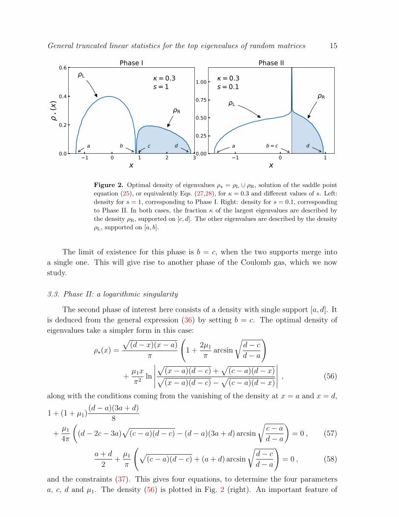
Figure 2. Optimal density of eigenvalues ρ? = ρL ∪ ρR, solution of the saddle point

equation (25), or equivalently Eqs. (27,28), for κ = 0.3 and different values of s. Left:

density for s = 1, corresponding to Phase I. Right: density for s = 0.1, corresponding

to Phase II. In both cases, the fraction κ of the largest eigenvalues are described by

the density ρR, supported on [c, d]. The other eigenvalues are described by the density

ρL, supported on [a, b].

The limit of existence for this phase is b = c, when the two supports merge into

a single one. This will give rise to another phase of the Coulomb gas, which we now

study.

3.3. Phase II: a logarithmic singularity

The second phase of interest here consists of a density with single support [a, d]. It

is deduced from the general expression (36) by setting b = c. The optimal density of

eigenvalues take a simpler form in this case:

ρ?(x) =

√(d− x)(x− a)

π

(1 +

2µ1

πarcsin

√d− cd− a

)

+µ1x

π2ln

∣∣∣∣∣√

(x− a)(d− c) +√

(c− a)(d− x)√(x− a)(d− c)−

√(c− a)(d− x)

∣∣∣∣∣ , (56)

along with the conditions coming from the vanishing of the density at x = a and x = d,

1 + (1 + µ1)(d− a)(3a+ d)

8

+µ1

4π

((d− 2c− 3a)

√(c− a)(d− c)− (d− a)(3a+ d) arcsin

√c− ad− a

)= 0 , (57)

a+ d

2+µ1

π

(√(c− a)(d− c) + (a+ d) arcsin

√d− cd− a

)= 0 , (58)

and the constraints (37). This gives four equations, to determine the four parameters

a, c, d and µ1. The density (56) is plotted in Fig. 2 (right). An important feature of

General truncated linear statistics for the top eigenvalues of random matrices 16

the density (56) is that is exhibits a logarithmic divergence at x = c:

ρ?(x) 'x→c−µ1c

π2ln |x− c| for c 6= 0 . (59)

This behaviour had already been found in [46] in the case of a monotonous linear

statistics. Additionally, when c = 0, the density no longer diverges, but presents a

different logarithmic singularity:

ρ?(x) 'x→c

√−adπ− µ1x

π2ln |x| for c = 0 . (60)

This type of singularity has, to the best of our knowledge, never been found previously

in the density of eigenvalues of random matrices. It arises here because of the non-

monotonicity of the function f in the truncated linear statistics (3).

A necessary condition for this phase to exist is that the density (56) should remain

positive for all x ∈ [a, d]. In particular, from the behaviour (59), this imposes that

µ1c > 0 . (61)

This is the complementary condition of the one obtained for Phase I, see Eq. (55).

Since the expression (56) for Phase II can be obtained by taking the limit b → c in

the general expressions of the density in Phase I (36), these two phases should share a

common boundary in the (κ, s) plane, which is thus given by µ1c = 0. This gives two

possibilities:

• µ1 = 0, which corresponds to the line s = s0(κ) in Fig. 1. This line was already

present in the case of monotonous functions studied in Ref. [46];

• c = 0, which gives a new line s = s1(κ) in the phase diagram (Fig. 1). As

we will discuss below, this line actually corresponds to the condition f ′(c) = 0.

The existence of this second line is thus specific to the study of truncated linear

statistics with a non monotonous function f .

Combining Eqs. (57,58) with the constraints (37), we can write this line c = 0

in the parametric form

κ =2

πarccos

(√−ad− a

), (62)

s1(κ) = (3d2 + 2ad+ 3a2 − 8)(−ad)3/2

16(a+ d)π, (63)

where a and d are related by

arccos

(√−ad− a

)+ (2 + ad)

√−ad

2(a+ d)= 0 . (64)

It has the following asymptotic behaviour

s1(κ) '

2π4κ5

45for κ→ 0 ,

3

2π2(1− κ)3for κ→ 1 .

(65)

Note that we can recover the condition (61) by reversing the physical argument

given in Section 3.2: the eigenvalues near x = c, for x > c, feel the force −µ1c. If this

force is positive, it pushes the eigenvalues to the right causing the opening of a gap. In

General truncated linear statistics for the top eigenvalues of random matrices 17

order to reverse the situation and get an accumulation of eigenvalues near x = c, as it

is the case here, this force must be negative. This condition yields (61).

3.4. Two infinite order phase transitions

We have seen that the two lines s0(κ) and s1(κ) delimit regions in the (κ, s) plane

in which the optimal density of eigenvalues ρ?(x;κ, s) takes different forms. We can

thus interpret these lines as phase transitions for the Coulomb gas. We now turn to the

analysis of the order of these transitions.

Line s0(κ) — We first consider the line on which µ1 = 0, corresponding to the most

probable value taken by the truncated linear statistics (3). On this line, the typical

density of eigenvalues is given by Wigner’s semicircle law. One can show that all the

derivatives of the energy of the Coulomb gas E [ρ?(x;κ, s)], and thus of the large deviation

function Φκ(s) are continuous on this line (see Appendix B). However, this function is

not analytic: it possesses an essential singularity in Phase I (corresponding to s = s+0

for κ < 12

and s = s−0 for κ > 12):

Φκ(s0(κ) + ε)− Φκ(s0(κ)− ε) = O(ε eγ0(κ)/ε) for κ 6= 1

2, (66)

where γ0(κ) is a constant. Therefore, in the standard terminology of statistical physics,

it corresponds to an infinite order phase transition. This exact same transition has been

observed in [46] for truncated linear statistics associated with a monotonous function f .

Here, we obtain exactly the same behavious for all values of κ 6= 12. Indeed, for these

values of κ, the typical position of the Kth largest eigenvalue (the last to contribute to s)

is λK 6= 0, away from the point where f has a minimum. Therefore, small fluctuations

of λK do not probe the non-monotonicity of f , and the behaviour of Φκ near s0(κ)

is identical to the one observed in the monotonous case, which has been shown to be

universal [46].

Line s1(κ) — The second line, corresponding to f ′(c) = 0 (that is, c = 0 here,

corresponding to κ = 12) is specific to the study of the case of non-monotonous functions

f . It is the main novelty that arises in this case.

On this line, the density presents a logarithmis singularity, as shown in Eq. (60). It

is a new specific feature to the case of truncated linear statistics with a non-monotonous

function f .

One can show (see Appendix B) that the large deviation function exhibits another

essential singularity on this line (again located in Phase I):

Φκ(s1(κ) + ε)− Φκ(s1(κ)− ε) = O(ε eγ1(κ)/ε) for κ 6= 1

2, (67)

where γ1(κ) is a constant. This shows that s1(κ) also corresponds to an infinite order

phase transition.

General truncated linear statistics for the top eigenvalues of random matrices 18

Intersection of the two lines for κ = 12

— The two phase transition lines intersect for

κ = 12. Indeed, for this specific value of κ, in the absence of constraint (µ1 = 0), the

Kth largest eigenvalue is typically located at 〈λK〉 = c = 0. At this point, the essential

singularities vanish, as well as the phase transition. Indeed, only Phase I exists for this

specific value of κ.

3.5. Distribution of the potential energy of the K rightmost fermions

Using the results above on the optimal density ρ?(x), we can study the distribution

of the truncated linear statistics under consideration: the potential energy of the K

rightmost fermions in a harmonic trap.

First cumulants — The value s0(κ) corresponds to the most probable value taken by

the truncated linear statistics, or equivalently by the potential energy of the K rightmost

fermions. It implies that

〈EP (K)〉 'N,K→∞

N2~ω2

s0(κ) ' ~ω2

2KN for K → 0 ,

2KN − 3

2N2 for K → N .

(68)

We can study the fluctuations around this value by expanding Eqs. (37,57,58) in the

limit µ1 → 0. We obtain

s = s0(κ) + F (c0)µ1 +O(µ21) , (69)

with

F (c0) =1

8π2

(3c4

0 − 14c20 − 4

√2− c2

0

(c2

0 − 1)c0 arccos

(c0√

2

)+ 4 arccos

(c0√

2

)2

+ 16

)(70)

and c0 is related to κ via (48). Inverting the series (69), we deduce the expression

of the large deviation function near s0(κ) via direct integration over s thanks to the

thermodynamic identity (24):

Φκ(s) 's→s0(κ)

(s− s0(κ))2

2F (c0)+O((s− s0(κ))3) . (71)

From this result, we straightforwardly deduce

Var(s) =2

βN2F (c0) ' 2

βN2

(

18

π

)2/3

κ4/3 for κ→ 0 ,

1

2− 4(1− κ) for κ→ 1 .

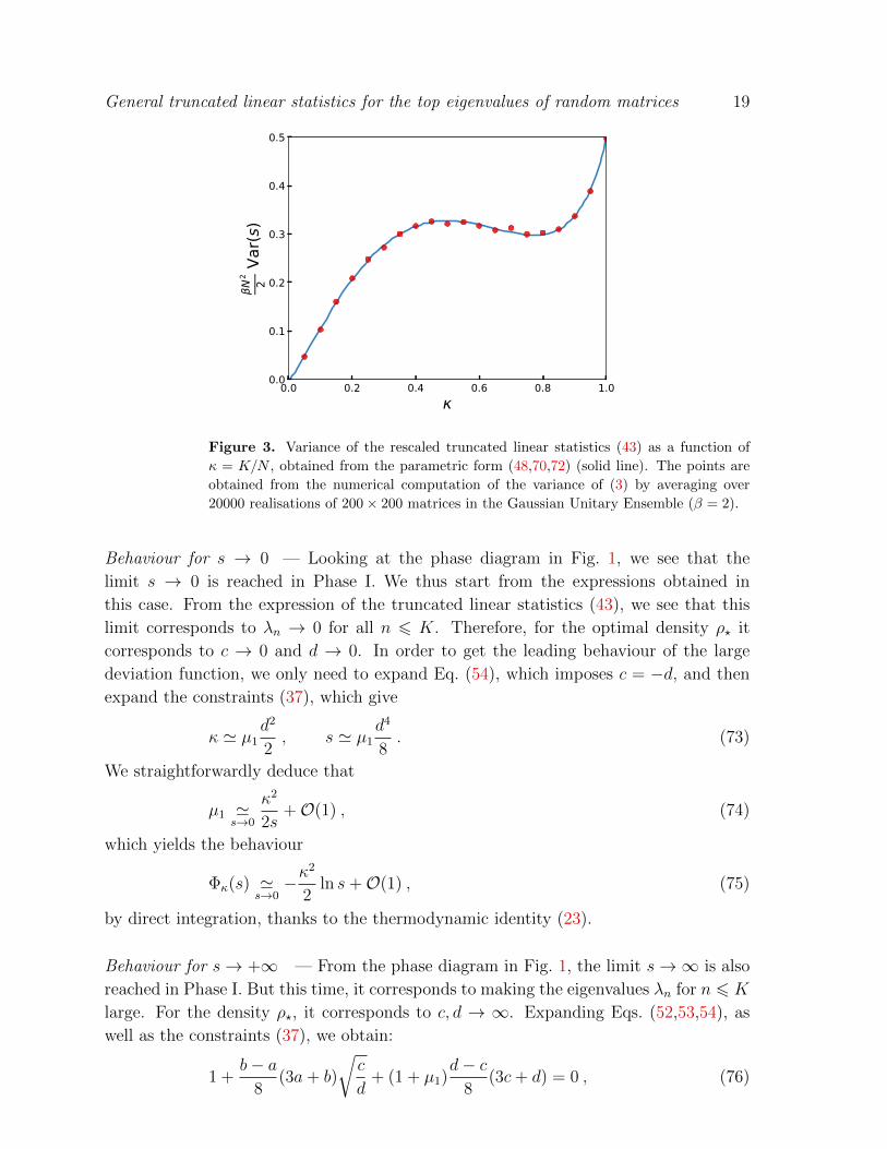
(72)

This variance is represented as a function of κ in Fig. 3. It displays a non-monotonic

behaviour, which has never been observed in previous studies on truncated linear

statistics [46, 51, 60]. This new feature has been confirmed by numerical simulations

(see Fig. 3).

General truncated linear statistics for the top eigenvalues of random matrices 19

0.0 0.2 0.4 0.6 0.8 1.00.0

0.1

0.2

0.3

0.4

0.5

N2 2

Var(s

)

Figure 3. Variance of the rescaled truncated linear statistics (43) as a function of

κ = K/N , obtained from the parametric form (48,70,72) (solid line). The points are

obtained from the numerical computation of the variance of (3) by averaging over

20000 realisations of 200× 200 matrices in the Gaussian Unitary Ensemble (β = 2).

Behaviour for s → 0 — Looking at the phase diagram in Fig. 1, we see that the

limit s → 0 is reached in Phase I. We thus start from the expressions obtained in

this case. From the expression of the truncated linear statistics (43), we see that this

limit corresponds to λn → 0 for all n 6 K. Therefore, for the optimal density ρ? it

corresponds to c → 0 and d → 0. In order to get the leading behaviour of the large

deviation function, we only need to expand Eq. (54), which imposes c = −d, and then

expand the constraints (37), which give

κ ' µ1d2

2, s ' µ1

d4

8. (73)

We straightforwardly deduce that

µ1 's→0

κ2

2s+O(1) , (74)

which yields the behaviour

Φκ(s) 's→0−κ

2

2ln s+O(1) , (75)

by direct integration, thanks to the thermodynamic identity (23).

Behaviour for s→ +∞ — From the phase diagram in Fig. 1, the limit s→∞ is also

reached in Phase I. But this time, it corresponds to making the eigenvalues λn for n 6 K

large. For the density ρ?, it corresponds to c, d → ∞. Expanding Eqs. (52,53,54), as

well as the constraints (37), we obtain:

1 +b− a

8(3a+ b)

√c

d+ (1 + µ1)

d− c8

(3c+ d) = 0 , (76)

General truncated linear statistics for the top eigenvalues of random matrices 20

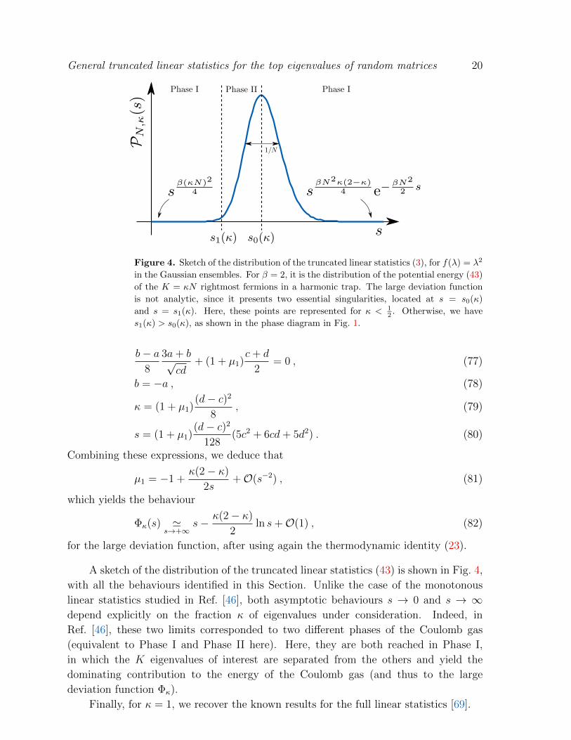
Figure 4. Sketch of the distribution of the truncated linear statistics (3), for f(λ) = λ2

in the Gaussian ensembles. For β = 2, it is the distribution of the potential energy (43)

of the K = κN rightmost fermions in a harmonic trap. The large deviation function

is not analytic, since it presents two essential singularities, located at s = s0(κ)

and s = s1(κ). Here, these points are represented for κ < 12 . Otherwise, we have

s1(κ) > s0(κ), as shown in the phase diagram in Fig. 1.

b− a8

3a+ b√cd

+ (1 + µ1)c+ d

2= 0 , (77)

b = −a , (78)

κ = (1 + µ1)(d− c)2

8, (79)

s = (1 + µ1)(d− c)2

128(5c2 + 6cd+ 5d2) . (80)

Combining these expressions, we deduce that

µ1 = −1 +κ(2− κ)

2s+O(s−2) , (81)

which yields the behaviour

Φκ(s) 's→+∞

s− κ(2− κ)

2ln s+O(1) , (82)

for the large deviation function, after using again the thermodynamic identity (23).

A sketch of the distribution of the truncated linear statistics (43) is shown in Fig. 4,

with all the behaviours identified in this Section. Unlike the case of the monotonous

linear statistics studied in Ref. [46], both asymptotic behaviours s → 0 and s → ∞depend explicitly on the fraction κ of eigenvalues under consideration. Indeed, in

Ref. [46], these two limits corresponded to two different phases of the Coulomb gas

(equivalent to Phase I and Phase II here). Here, they are both reached in Phase I,

in which the K eigenvalues of interest are separated from the others and yield the

dominating contribution to the energy of the Coulomb gas (and thus to the large

deviation function Φκ).

Finally, for κ = 1, we recover the known results for the full linear statistics [69].

General truncated linear statistics for the top eigenvalues of random matrices 21

4. Universality

In Section 3 we have applied the Coulomb gas formalism to the study of an example

of truncated linear statistics with a non monotonous function f , motivated by the study

of a gas of cold fermions. We now argue that several features of the Coulomb gas, and

thus of the large deviation function, are actually universal in the sense that they do

not depend on the specific choice of the linear statistics (i.e. the function f) or on the

matrix ensemble (i.e. the potential V ). Let us again denote ρ0 the typical density of

eigenvalues in the ensemble under consideration, and c0(κ) = 〈λκN〉 the position of the

smallest eigenvalue to contribute to the truncated linear statistics (3). This position

can be determined from ρ0 via the relation

κ =

∫c0(κ)

ρ0(x)dx . (83)

The following features are expected to occur in the study of any truncated linear

statistics.

• The line s0(κ), corresponding to µ1 = 0, gives the typical value of the truncated

linear statistics restricted to the fraction κ of the largest eigenvalues. It is shown

in Appendix B that this line also corresponds to a transition line between two

phases: a phase in which the density is supported on two disjoint supports

(Phase I), and one in which the density exhibits a logarithmic divergence

(Phase II). Moreover, it corresponds to an infinite order phase transition for

all values of κ such that f ′(c0(κ)) 6= 0. This extends the results of Ref. [46] to

the case of a non-monotonous function f .

• The line s1(κ) is also present for any non-monotonous function f , at least in

the vicinity of the typical line s0(κ). Indeed, away from this line, the two

phases studied in this article could stop to exist and let other configurations

of the Coulomb gas emerge (such as densities with more than two supports).

Nevertheless, for values of s close to s0(κ), the line s1(κ) is expected to exist,

and is also an infinite order phase transition for the Coulomb gas, as is shown

in Appendix B.

• The two lines s0(κ) and s1(κ) intersect for values of κ which verify f ′(c0(κ)) = 0.

There are as many intersections as local extrema of the function f in the support

of ρ0. At these points, there is no longer a phase transition in the Coulomb gas,

as it remains in the same phase both for s < s0(κ) and s > s0(κ).

• The positions of Phase I and Phase II with respect to the line s0(κ) are

exchanged after a crossing with the line s1(κ).

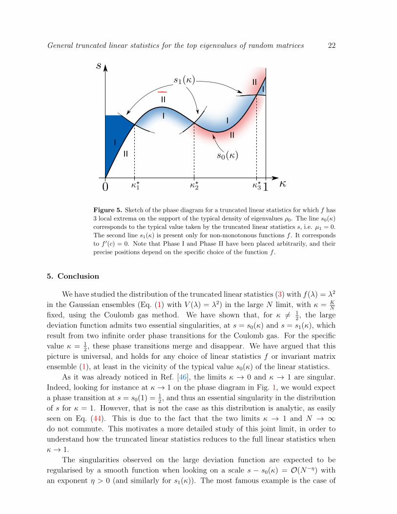
We show in Fig. 5 a sketch of the corresponding phase diagram of the Coulomb gas, in

the vicinity of the line s0(κ), in the case where the lines s0(κ) and s1(κ) intersect for 3

different values of κ.

General truncated linear statistics for the top eigenvalues of random matrices 22

Figure 5. Sketch of the phase diagram for a truncated linear statistics for which f has

3 local extrema on the support of the typical density of eigenvalues ρ0. The line s0(κ)

corresponds to the typical value taken by the truncated linear statistics s, i.e. µ1 = 0.

The second line s1(κ) is present only for non-monotonous functions f . It corresponds

to f ′(c) = 0. Note that Phase I and Phase II have been placed arbitrarily, and their

precise positions depend on the specific choice of the function f .

5. Conclusion

We have studied the distribution of the truncated linear statistics (3) with f(λ) = λ2

in the Gaussian ensembles (Eq. (1) with V (λ) = λ2) in the large N limit, with κ = KN

fixed, using the Coulomb gas method. We have shown that, for κ 6= 12, the large

deviation function admits two essential singularities, at s = s0(κ) and s = s1(κ), which

result from two infinite order phase transitions for the Coulomb gas. For the specific

value κ = 12, these phase transitions merge and disappear. We have argued that this

picture is universal, and holds for any choice of linear statistics f or invariant matrix

ensemble (1), at least in the vicinity of the typical value s0(κ) of the linear statistics.

As it was already noticed in Ref. [46], the limits κ → 0 and κ → 1 are singular.

Indeed, looking for instance at κ→ 1 on the phase diagram in Fig. 1, we would expect

a phase transition at s = s0(1) = 12, and thus an essential singularity in the distribution

of s for κ = 1. However, that is not the case as this distribution is analytic, as easily

seen on Eq. (44). This is due to the fact that the two limits κ → 1 and N → ∞do not commute. This motivates a more detailed study of this joint limit, in order to

understand how the truncated linear statistics reduces to the full linear statistics when

κ→ 1.

The singularities observed on the large deviation function are expected to be

regularised by a smooth function when looking on a scale s − s0(κ) = O(N−η) with

an exponent η > 0 (and similarly for s1(κ)). The most famous example is the case of

General truncated linear statistics for the top eigenvalues of random matrices 23

the largest eigenvalue: its large deviation function displays a singularity which originates

from a third order phase transition for the Coulomb gas when looking at fluctuations

of order λmax − 〈λmax〉 = O(1) (for the distribution (1) for which λn = O(N0) ). This

singularity is regularised when looking on a scale ∆λ = λmax − 〈λmax〉 = O(N−2/3),

where ∆λ obeys the Tracy-Widom distribution [58]. We expect an equivalent function

here that regularises the distribution of the truncated linear statistics at s0(κ) and

s1(κ), when looking on a smaller scale. It would be of particular interest to study the

behaviour of this function in vicinity of the point(s) where the two phase transition

lines s0(κ) and s1(κ) intersect, as there is no singular behaviour at this point. It could

thus help to understand how these essential singularities emerge in the distribution of

truncated linear statistics.

Appendix A. A few useful integrals

The following integrals are used in the manuscript.

−∫ b

a

dt

π

√(t− a)(b− t)t− x

1

t− y= −1 +

√(y − a)(y − b)|y − x|

, x ∈ [a, b] , y /∈ [a, b] , (A.1)

−∫ b

a

dt

π

1

(x− t)√

(t− a)(b− t)=

− 1√

(a− x)(b− x), x < a

0 , a < x < b

1√(x− a)(x− b)

, x > b

(A.2)

Appendix B. Infinite order phase transitions

We interpret the two lines s0(κ) and s1(κ) as phase transitions lines for the Coulomb

gas. We now show that these transitions are of infinite order, for any invariant matrix

ensemble (choice of V ) and any linear statistics (f). A similar analysis was performed

in Ref. [46] in the Laguerre ensembles (see Table 1), and for a monotonous function f .

We extend this discussion to the general case, and in particular to the study of the line

s1(κ) which emerges due to the non-monotony of f .

Let us start from the general expression of the density (36). It depends on

five parameters: a, b, c, d and µ1. These parameters are determined by the two

constraints (37), along with conditions on the boundaries a, b and d of the support

(the condition at x = c has already been used in the derivation of the expression (36)

for the density). The determination of the value of b depends on the phase we consider:

• In Phase I in which the supports are disjoint (b < c), the value of b is determined

by imposing that the density does not diverge as (b − x)−1/2 for x → b− (as it

was done for c), since this kind of behaviour only appears near a hard edge.

This gives

2 =

∫ b

a

dt

πV ′(t)

√(t− a)(d− t)(b− t)(c− t)

−∫ d

c

dt

π(V ′(t) +µ1f

′(t))

√(t− a)(d− t)(t− b)(t− c)

.(B.1)

General truncated linear statistics for the top eigenvalues of random matrices 24

• In Phase II, b is directly obtained as b = c.

There remains to determine the outer edges a and d. There are different

possibilities, depending on the random matrix ensemble under consideration (and hence

on the choice of V ). In the main text, since we worked in the Gaussian ensembles, we

imposed that the density vanishes at x = a and x = d. In general, these conditions take

the form

2 +

∫[a,b]∪[c,d]

dt

π(V ′(t) + µ1f

′(t)Θ(t− c))

√(b− t)(d− t)(t− a)(c− t)

= 0 , (B.2)

2−∫

[a,b]∪[c,d]

dt

π(V ′(t) + µ1f

′(t)Θ(t− c))

√(b− t)(t− a)

(c− t)(d− t)= 0 . (B.3)

Note that other types of boundary conditions can apply. For instance, in the Jacobi

ensembles in which the eigenvalues are restricted to [0, 1] (see Table 1), we could have

instead the conditions a = 0 and d = 1. In the following, we will consider only the case

where the density vanishes at x = a and x = d, and thus we impose (B.2,B.3), since the

following procedure can be straightforwardly adapted to the other types of boundary

conditions.

In order to analyse the order of the two transitions occuring at s = s0(κ) and

s = s1(κ), we study the behaviour of

Φκ(s0(κ) + ε)− Φκ(s0(κ)− ε) and Φκ(s1(κ) + ε)− Φκ(s1(κ)− ε) (B.4)

for ε → 0. The two lines s0(κ) and s1(κ) corresponding to transitions between Phase

I and Phase II, the limit ε → 0 in Phase I corresponds to the limit b → c in both

cases. Expanding the conditions on a, b and d (B.1,B.2,B.3) in this limit, we obtain for

Phase I:

µ1f′(c) =

α

ln(c− b)⇒ c− b = eα/(µ1f

′(c)) , (B.5)

2 +

∫ d

a

dt

π(V ′(t) + µ1f

′(t)Θ(t− c))√d− tt− a

= O(

eα/(µ1f′(c))

µ1f ′(c)

), (B.6)

2−∫ d

a

dt

π(V ′(t) + µ1f

′(t)Θ(t− c))√t− ad− t

= O(

eα/(µ1f′(c))

µ1f ′(c)

), (B.7)

where we have denoted

α =π√

(c− a)(d− c)

(2 +−

∫ d

a

dt

π

V ′(t)

t− c√

(t− a)(d− t)). (B.8)

Similarly, using the expression of the density (36), the constraints (37) take the form:

κ =

∫ d

c

dx

2π

1√(x− a)(d− x)

{2 +

∫ d

a

dt

π

V ′(t)

t− x√

(t− a)(d− t)

+ µ1

∫ d

c

dt

π

f ′(t)

t− x√

(t− a)(d− t)}

+O(

eα/(µ1f′(c))

µ1f ′(c)

), (B.9)

General truncated linear statistics for the top eigenvalues of random matrices 25

s =

∫ d

c

dx

2π

f(x)√(x− a)(d− x)

{2 +

∫ d

a

dt

π

V ′(t)

t− x√

(t− a)(d− t)

+ µ1

∫ d

c

dt

π

f ′(t)

t− x√

(t− a)(d− t)}

+O(

eα/(µ1f′(c))

µ1f ′(c)

). (B.10)

In Phase II, we obtain exactly the same expressions but without the terms in

O(eα/(µ1f′(c))/(µ1f

′(c))). From these expressions, we now consider each transition line

independently.

Line s0(κ): µ1 = 0 — Let us first study the transition occuring on the line s0(κ). It

corresponds to µ1 = 0 and hence the most probable value of the linear statistics. It is

given in a parametric form by

s0(κ) =

∫ d0

c0

f(x)ρ0(x)dx , κ =

∫ d0

c0

ρ0(x)dx (B.11)

in terms of the position c0 = 〈λK〉 of the last eigenvalue to contribute to s, where we

have denoted

ρ0(x) =1

π√

(x− a)(d− x)

(1 +−

∫ d

a

dt

2π

V ′(t)

t− x√

(t− a)(d− t))

(B.12)

the typical density of eigenvalues in the absence of constraint.

For values of c0 such that f ′(c0) 6= 0, Eqs. (B.6,B.7,B.9,B.10) are identical to the

ones studied in Ref. [46] in the case of a monotonous linear statistics. The fact that we

recover these exact same equations can be understood as follows: the small fluctuations

of λK around the typical value c0 are not sufficient to probe the non-monotony of f if

f ′(c0) 6= 0. Therefore, for these values, the line s0(κ) corresponds to an infinite order

phase transition, as it was shown in Ref. [46]. The idea to prove this result is to expand

Eqs. (B.6,B.7,B.9,B.10) for s → s0(κ), i.e. for µ1 → 0, and combine them in order to

get

s− s0(κ) = F0(κ)µ1 +O(µ21) +O

(eα/(µ1f

′(c0))

µ1

)(Phase I) , (B.13)

s− s0(κ) = F0(κ)µ1 +O(µ21) (Phase II) . (B.14)

where F0(κ) is a constant fully determined by this expansion. For the case considered

in the main text (f(x) = V (x) = x2), F0 is given parametrically by (48,70). For the

expansion in Phase I, we have kept the subleading term O(

eα/(µ1f′(c0))

µ1

), as it is the

only one which differs from the expansion in Phase II, since all the terms in O(µn1 ) are

identical in both expressions. Inverting these expansions, we obtain µ1 as a function

of s, which can be integrated to yield Φκ(s) by using the thermodynamic identity (24).

This gives

d

dε[Φκ(s0(κ) + ε)− Φκ(s0(κ)− ε)] = O(eγ0(κ)/ε/ε) , (B.15)

which after integration becomes

Φκ(s0(κ) + ε)− Φκ(s0(κ)− ε) = O(ε eγ0(κ)/ε) , (B.16)

General truncated linear statistics for the top eigenvalues of random matrices 26

where we have denoted

γ0(κ) =α

f ′(c0)F0(κ) , (B.17)

with c0 determined from κ via (B.11). This proves that all the derivatives of Φκ are

continuous on the line s0(κ), but the function is not analytic at this point, due to

the essential singularity present in Phase I. However, for specific values of κ such that

f ′(c0) = 0 this singularity vanishes and there is no transition. Indeed, the optimal

density of eigenvalues is given by the one of Phase I in both cases s > s0(κ) and

s < s0(κ) (see for instance Fig. 1 for κ = 12).

Line s1(κ): f ′(c) = 0 — We now turn to the case of the second transition line,

which is specific to the study of non-monotonous truncated linear statistics. The

behaviour of the large deviation function for s near s1(κ) can be obtained in Phase I

from (B.6,B.7,B.9,B.10) by expanding these equations around c = c such that f ′(c) = 0.

For c = c, we have µ1 = µ1. For µ1 6= 0, we can combine these expansions in order to

write (B.10) as

s− s1(κ) = F1(κ)(µ1 − µ1) +O((µ1 − µ1)2) +O(

eγ1(κ)/(µ1−µ1)

µ1 − µ1

)(Phase I) , (B.18)

where F1(κ) and γ1(κ) are two constants. We have kept the subleading last term, as for

Phase II, we have the same expansion, but without this last term:

s− s1(κ) = F1(κ)(µ1 − µ1) +O((µ1 − µ1)2) (Phase II) . (B.19)

In these two expansions all the regular powers O((µ1 − µ1)n) are identical, the only

difference is the essential singularity present in Phase I only. The large deviations

function can be deduced from these expansions via the thermodynamic identity (23),

which yields

d

dε[Φκ(s1(κ) + ε)− Φκ(s1(κ)− ε)] = O(eγ1(κ)/ε/ε) , (B.20)

which after integration gives

Φκ(s1(κ) + ε)− Φκ(s1(κ)− ε) = O(ε eγ1(κ)/ε) , (B.21)

where we have denoted γ1(κ) = F1(κ)γ1(κ). This proves that the line s1(κ) is also

associated to an infinite order phase transition.

References

[1] E. P. Wigner, On the statistical distribution of the widths and spacings of nuclear resonance

levels, Math. Proc. Cambridge Philos. Soc. 47(4), 790–798 (1951).

[2] C. W. J. Beenakker, Random-matrix theory of quantum transport, Rev. Mod. Phys. 69, 731–808

(1997).

[3] T. Guhr, A. Muller-Groeling, and H. A. Weidenmuller, Random-matrix theories in quantum

physics: common concepts, Phys. Rep. 299(4/6), 189–425 (1998).

[4] I. L. Aleiner, P. W. Brouwer, and L. I. Glazman, Quantum effects in Coulomb blockade, Phys.

Rep. 358(5-6), 309–440 (2002).

General truncated linear statistics for the top eigenvalues of random matrices 27

[5] P. A. Mello and N. Kumar, Quantum transport in mesoscopic systems – Complexity and statistical

fluctuations, Oxford University Press, 2004.

[6] P. W. Brouwer, Generalized circular ensemble of scattering matrices for a chaotic cavity with

nonideal leads, Phys. Rev. B 51, 16878–16884 (1995).

[7] P. A. Mello and H. U. Baranger, Interference phenomena in electronic transport through chaotic

cavities: An information-theoretic approach, Waves Random Media 9, 105–162 (1999).

[8] H.-J. Sommers, W. Wieczorek, and D. V. Savin, Statistics of conductance and shot noise power

for chaotic cavities, Acta Phys. Pol. A 112, 691 (2007).

[9] P. Vivo, S. N. Majumdar, and O. Bohigas, Distributions of Conductance and Shot Noise and

Associated Phase Transitions, Phys. Rev. Lett. 101, 216809 (2008).

[10] B. A. Khoruzhenko, D. V. Savin, and H.-J. Sommers, Systematic approach to statistics of

conductance and shot-noise in chaotic cavities, Phys. Rev. B 80, 125301 (2009).

[11] P. Vivo, S. N. Majumdar, and O. Bohigas, Probability distributions of linear statistics in chaotic

cavities and associated phase transitions, Phys. Rev. B 81, 104202 (2010).

[12] P. Vivo and E. Vivo, Transmission eigenvalue densities and moments in chaotic cavities from

random matrix theory, J. Phys. A: Math. Theor. 41(12), 122004 (2008).

[13] A. Grabsch and C. Texier, Capacitance and charge relaxation resistance of chaotic cavities—Joint

distribution of two linear statistics in the Laguerre ensemble of random matrices, Europhys.

Lett. 109(5), 50004 (2015).

[14] F. D. Cunden, P. Facchi, and P. Vivo, Joint statistics of quantum transport in chaotic cavities,

Europhys. Lett. 110(5), 50002 (2015).

[15] D. N. Page, Average entropy of a subsystem, Phys. Rev. Lett. 71, 1291–1294 (1993).

[16] P. Facchi, U. Marzolino, G. Parisi, S. Pascazio, and A. Scardicchio, Phase Transitions of Bipartite

Entanglement, Phys. Rev. Lett. 101, 050502 (2008).

[17] A. De Pasquale, P. Facchi, G. Parisi, S. Pascazio, and A. Scardicchio, Phase transitions and

metastability in the distribution of the bipartite entanglement of a large quantum system, Phys.

Rev. A 81, 052324 (2010).

[18] C. Nadal, S. N. Majumdar, and M. Vergassola, Phase Transitions in the Distribution of Bipartite

Entanglement of a Random Pure State, Phys. Rev. Lett. 104, 110501 (2010).

[19] C. Nadal, S. N. Majumdar, and M. Vergassola, Statistical Distribution of Quantum Entanglement

for a Random Bipartite State, J. Stat. Phys. 142(2), 403–438 (2011).

[20] P. Facchi, G. Florio, G. Parisi, S. Pascazio, and K. Yuasa, Entropy-driven phase transitions of

entanglement, Phys. Rev. A 87, 052324 (2013).

[21] C. Nadal and S. N. Majumdar, Nonintersecting Brownian interfaces and Wishart random matrices,

Phys. Rev. E 79, 061117 (2009).

[22] C. Nadal, Matrices aleatoires et leurs applications a la physique statistique et physique quantique,

PhD thesis, Universite Paris-Sud, 2011.

[23] R. Marino, S. N. Majumdar, G. Schehr, and P. Vivo, Number statistics for β-ensembles of random

matrices: applications to trapped fermions at zero temperature, Phys. Rev. E 94, 032115 (2016).

[24] D. S. Dean, P. L. Doussal, S. N. Majumdar, and G. Schehr, Noninteracting fermions in a trap

and random matrix theory, J. Phys. A: Math. Theor. 52(14), 144006 (2019).

[25] M. L. Mehta, Random matrices, Elsevier, Academic, New York, third edition, 2004.

[26] P. J. Forrester, Log-gases and random matrices, Princeton University Press, 2010.

[27] G. Akemann, J. Baik, and P. Di Francesco, The Oxford handbook of random matrix theory, Oxford

University Press, 2011.

[28] S. N. Majumdar, C. Nadal, A. Scardicchio, and P. Vivo, Index distribution of Gaussian random

matrices, Phys. Rev. Lett. 103, 220603 (2009).

[29] S. N. Majumdar, C. Nadal, A. Scardicchio, and P. Vivo, How many eigenvalues of a Gaussian

random matrix are positive?, Phys. Rev. E 83, 041105 (2011).

[30] S. N. Majumdar and P. Vivo, Number of Relevant Directions in Principal Component Analysis

and Wishart Random Matrices, Phys. Rev. Lett. 108, 200601 (2012).

General truncated linear statistics for the top eigenvalues of random matrices 28

[31] R. Marino, S. N. Majumdar, G. Schehr, and P. Vivo, Index distribution of Cauchy random

matrices, J. Phys. A: Math. Theor. 47(5), 055001 (2014).

[32] R. Marino, S. N. Majumdar, G. Schehr, and P. Vivo, Phase Transitions and Edge Scaling of

Number Variance in Gaussian Random Matrices, Phys. Rev. Lett. 112, 254101 (2014).

[33] P. Kazakopoulos, P. Mertikopoulos, A. L. Moustakas, and G. Caire, Living at the Edge: A Large

Deviations Approach to the Outage MIMO Capacity, IEEE Trans. Info. Theo. 57(4), 1984–2007

(2011).

[34] A. Karadimitrakis, A. L. Moustakas, and P. Vivo, Outage Capacity for the Optical MIMO

Channel, IEEE Trans. Info. Theo. 60(7), 4370–4382 (2014).

[35] F. J. Dyson and M. L. Mehta, Statistical Theory of the Energy Levels of Complex Systems. IV,

J. Math. Phys. 4(5), 701–712 (1963).

[36] C. W. J. Beenakker, Universality in the random-matrix theory of quantum transport, Phys. Rev.

Lett. 70, 1155–1158 (1993).

[37] C. W. J. Beenakker, Random-matrix theory of mesoscopic fluctuations in conductors and

superconductors, Phys. Rev. B 47, 15763–15775 (1993).

[38] C. Beenakker, Universality of Brezin and Zee’s spectral correlator, Nucl. Phys. B 422(3), 515 –

520 (1994).

[39] E. L. Basor and C. A. Tracy, Variance calculations and the Bessel kernel, J. Stat. Phys. 73(1),

415–421 (1993).

[40] B. Jancovici and P. J. Forrester, Derivation of an asymptotic expression in Beenakker’s general

fluctuation formula for random-matrix correlations near an edge, Phys. Rev. B 50, 14599–14600

(1994).

[41] D. S. Dean and S. N. Majumdar, Large Deviations of Extreme Eigenvalues of Random Matrices,

Phys. Rev. Lett. 97, 160201 (2006).

[42] P. Vivo, S. N. Majumdar, and O. Bohigas, Large deviations of the maximum eigenvalue in Wishart

random matrices, J. Phys. A: Math. Theor. 40(16), 4317 (2007).

[43] F. J. Dyson, Statistical Theory of the Energy Levels of Complex Systems. I, J. Math. Phys. 3(1),

140–156 (1962),

F. J. Dyson, Statistical Theory of the Energy Levels of Complex Systems. II, J. Math. Phys.

3(1), 157–165 (1962),

F. J. Dyson,Statistical Theory of the Energy Levels of Complex Systems. III, J. Math. Phys.

3(1), 166–175 (1962).

[44] G. Ben Arous and A. Guionnet, Large deviations for Wigner’s law and Voiculescu’s non-

commutative entropy, Prob. Theo. Relat. Fields 108(4), 517–542 (1997).

[45] G. Ben Arous and O. Zeitouni, Large deviations from the circular law, ESAIM: Prob. Stat. 2,

123–134 (1998).

[46] A. Grabsch, S. N. Majumdar, and C. Texier, Truncated Linear Statistics Associated with the

Top Eigenvalues of Random Matrices, J. Stat. Phys. 167(2), 234–259 (2017), updated version

arXiv:1609.08296.

[47] O. Bohigas and M. P. Pato, Randomly incomplete spectra and intermediate statistics, Phys. Rev.

E 74, 036212 (2006).

[48] T. Berggren and M. Duits, Mesoscopic Fluctuations for the Thinned Circular Unitary Ensemble,

Math. Phys. Anal. Geom. 20(3), 19 (2017).

[49] C. Charlier and T. Claeys, Thinning and conditioning of the circular unitary ensemble, Random

Matrices: Theory Appl. 06(02), 1750007 (2017).

[50] G. Lambert, Incomplete determinantal processes: from random matrix to Poisson statistics,

preprint arXiv:1612.00806 (2016).

[51] A. Grabsch, S. N. Majumdar, and C. Texier, Truncated Linear Statistics Associated with the

Eigenvalues of Random Matrices II. Partial Sums over Proper Time Delays for Chaotic Quantum

Dots, J. Stat. Phys. 167(6), 1452–1488 (2017).

[52] L. I. Smith, A tutorial on principal components analysis, 2002.

General truncated linear statistics for the top eigenvalues of random matrices 29

[53] C. A. Tracy and H. Widom, Level-spacing distributions and the Airy kernel, Commun. Math.

Phys. 159(1), 151–174 (1994).

[54] C. A. Tracy and H. Widom, On orthogonal and symplectic matrix ensembles, Commun. Math.

Phys. 177(3), 727–754 (1996).

[55] K. Johansson, From Gumbel to Tracy-Widom, Probab. Theory Rel. 138(1), 75–112 (2007).

[56] D. S. Dean and S. N. Majumdar, Extreme value statistics of eigenvalues of Gaussian random

matrices, Phys. Rev. E 77, 041108 (2008).

[57] G. Borot, B. Eynard, S. N. Majumdar, and C. Nadal, Large deviations of the maximal eigenvalue

of random matrices, J. Stat. Mech: Theory Exp. 2011(11), P11024 (2011).

[58] S. N. Majumdar and G. Schehr, Top eigenvalue of a random matrix: large deviations and third

order phase transition, J. Stat. Mech. 2014(1), P01012 (2014).

[59] A. Krajenbrink and P. L. Doussal, Linear statistics and pushed Coulomb gas at the edge of β

-random matrices: Four paths to large deviations, Europhy. Lett. 125(2), 20009 (2019).

[60] A. Flack, S. N. Majumdar, and G. Schehr, Truncated linear statistics in the one dimensional

one-component plasma, J. Phys. A: Math. Theor. 54(43), 435002 (2021).

[61] F. J. Dyson, The Threefold Way. Algebraic Structure of Symmetry Groups and Ensembles in

Quantum Mechanics, J. Math. Phys. 3, 1199–1215 (1962).

[62] F. D. Cunden, P. Facchi, and P. Vivo, A shortcut through the Coulomb gas method for spectral

linear statistics on random matrices, J. Phys. A: Math. Theor. 49(13), 135202 (2016).

[63] A. Grabsch and C. Texier, Distribution of spectral linear statistics on random matrices beyond

the large deviation function – Wigner time delay in multichannel disordered wires, J. Phys. A:

Math. Theor. 49, 465002 (2016).

[64] F. G. Tricomi, Integral equations, Interscience, London, 1957.

[65] D. S. Dean, P. L. Doussal, S. N. Majumdar, and G. Schehr, Universal ground-state properties of

free fermions in a d -dimensional trap, Europhys. Lett. 112(6), 60001 (2015).

[66] D. S. Dean, P. Le Doussal, S. N. Majumdar, and G. Schehr, Finite-Temperature Free Fermions

and the Kardar-Parisi-Zhang Equation at Finite Time, Phys. Rev. Lett. 114, 110402 (2015).

[67] D. S. Dean, P. Le Doussal, S. N. Majumdar, and G. Schehr, Noninteracting fermions at finite

temperature in a d-dimensional trap: Universal correlations, Phys. Rev. A 94, 063622 (2016).

[68] A. Grabsch, S. N. Majumdar, G. Schehr, and C. Texier, Fluctuations of observables for free

fermions in a harmonic trap at finite temperature, SciPost Phys. 4, 014 (2018).

[69] J. Grela, S. N. Majumdar, and G. Schehr, Kinetic Energy of a Trapped Fermi Gas at Finite

Temperature, Phys. Rev. Lett. 119, 130601 (2017).