
Statistics Worksheet for Statistics and Research Methods in Psychology course
41
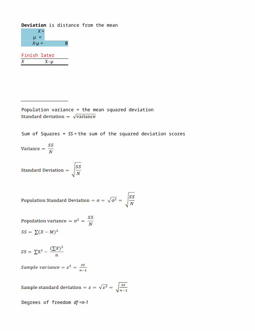
X = μ = 0 Finish later X Population variance = the mean squared deviation Deviation is distance from the mean X-μ = X-μ Sum of Squares = SS = the sum of the squared deviation scores Degrees of freedom df =n-1
description
I made this "cheat sheet" to help me keep my calculations and work organized rather than use a pen and paper. I also helped me to check my work. It's not pretty and I may be the only person that can read it well but generally you just plug in numbers to the grey boxes and the calculations will take care of themselves. I spent a lot of time on this so I hope somebody else can get some use out of it. Enjoy!
Transcript of Statistics Worksheet for Statistics and Research Methods in Psychology course
X =μ =
0
Finish laterX
Population variance = the mean squared deviation
Deviation is distance from the mean
X-μ =
X-μ
Sum of Squares = SS = the sum of the squared deviation scores
Degrees of freedom df =n-1

Z-score for a sample
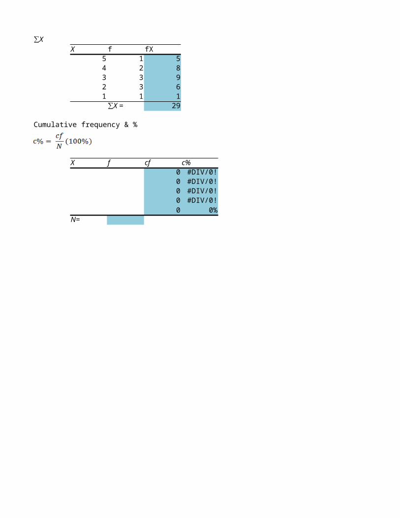
X f fX5 1 54 2 83 3 92 3 61 1 1
29
Cumulative frequency & %
X f cf c%0 #DIV/0!0 #DIV/0!0 #DIV/0!0 #DIV/0!0 0%
N=
∑X
∑X =

Cohen's d


Ch7
Standard error
Z-score sample means

6
Z-score -
binomial distributionp(A) = p and p(B) = q
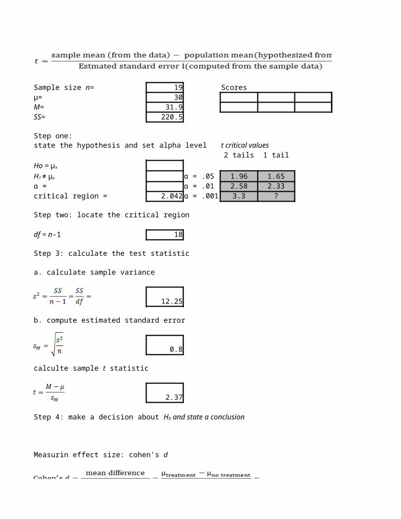
19 Scoresμ= 30M= 31.9SS= 220.5
Step one: state the hypothesis and set alpha level t critical values
2 tails 1 tail α = .05 1.96 1.65
α = α = .01 2.58 2.33critical region = 2.042 α = .001 3.3 ?
Step two: locate the critical region
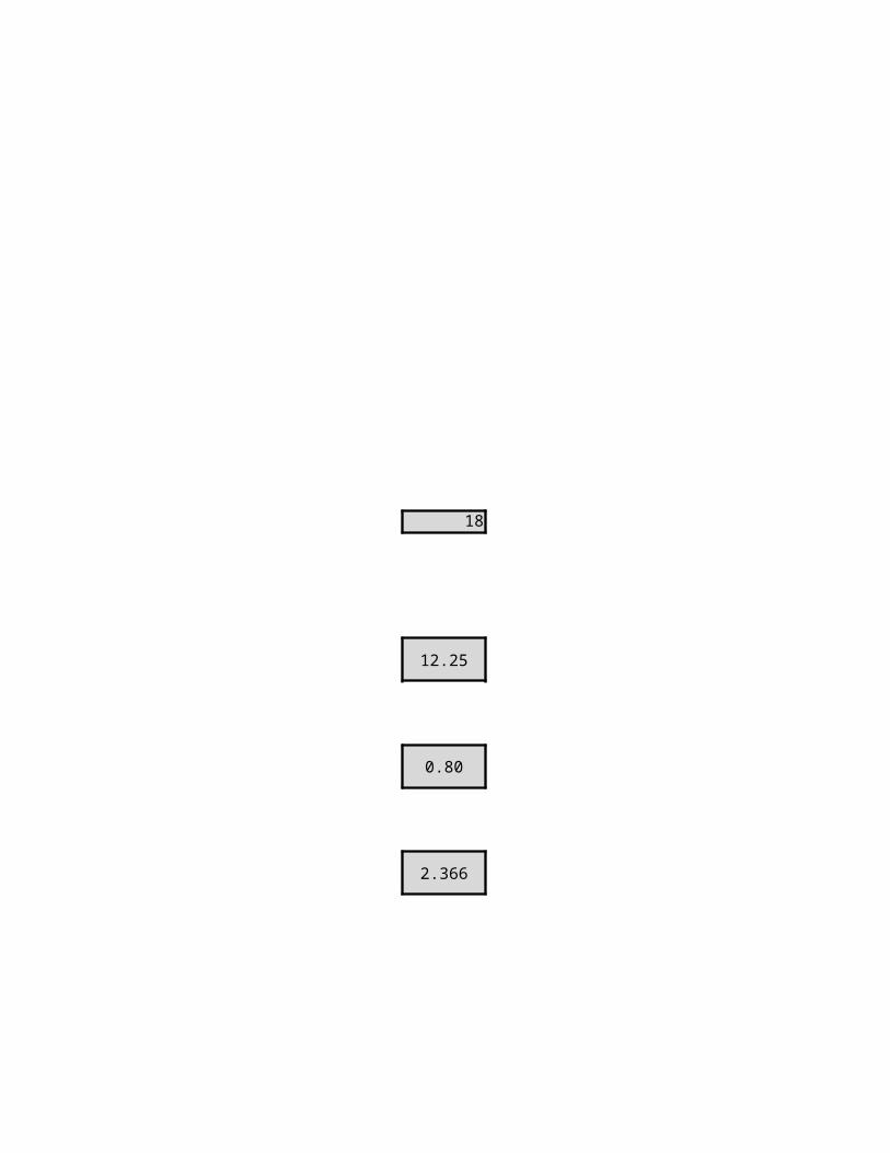
18
Step 3: calculate the test statistic
a. calculate sample variance
12.25
b. compute estimated standard error
0.8
2.37
Sample size n=
Ho = μx
H1 ≠ μx
df = n-1
calculte sample t statistic
Step 4: make a decision about H0 and state a conclusion
Measurin effect size: cohen's d
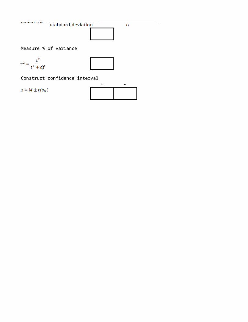
Measure % of variance
Construct confidence interval+ -

18
12.25
0.80
2.366
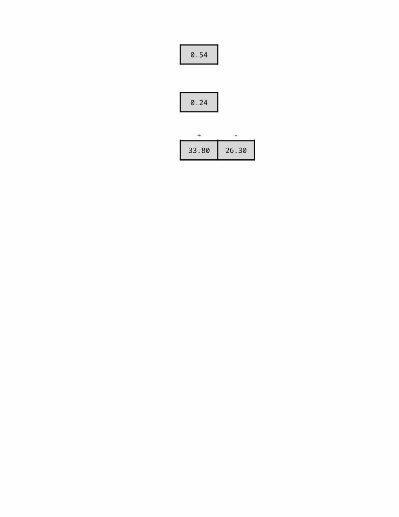
0.54
0.24
+ -
33.80 26.30
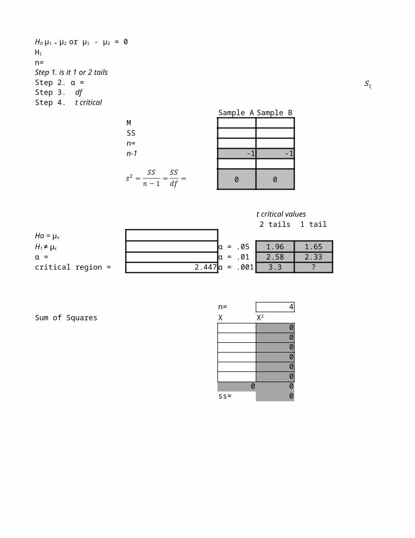
n= Estimated standard errorStep 1. is it 1 or 2 tailsStep 2. α =
Pooled varianceSample A Sample B
MSS t - statistic
n=n-1 -1 -1
0 0
Confidence intervalt critical values
2 tails 1 tail F-max α = .05 1.96 1.65
α = α = .01 2.58 2.33 r^2critical region = 2.447 α = .001 3.3 ?
n= 4Sum of Squares X
000000
0 0ss= 0
H0: μ1 = μ2 or μ1 - μ2 = 0H1
Step 3. dfStep 4. t critical
Cohen's d
Ho = μx
H1 ≠ μx
X2
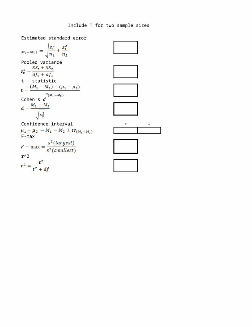
Include T for two sample sizes
Estimated standard error
Pooled variance
t - statistic
Confidence interval + -
#DIV/0!
0
#DIV/0!
#DIV/0!
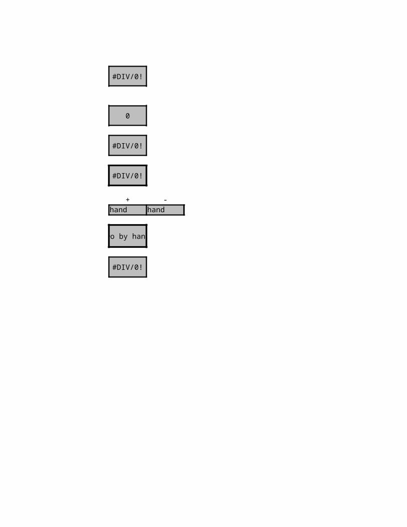
+hand
Do by hand
#DIV/0!
-hand
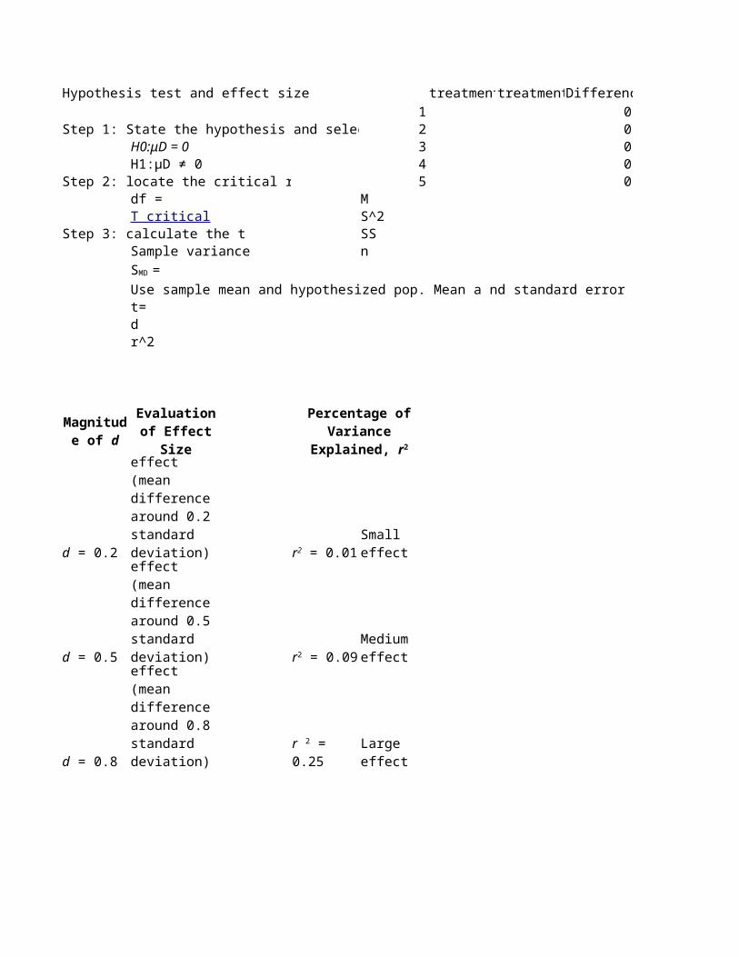
Hypothesis test and effect size treatment treatment Difference1 0 0
Step 1: State the hypothesis and select alpha 2 0 0H0:μD = 0 3 0 0
4 0 0Step 2: locate the critical region 5 0 0
df = M S^2
Step 3: calculate the t SSSample variance n
Use sample mean and hypothesized pop. Mean a nd standard error to compute t statt=d r^2
D2
H1:μD ≠ 0
T critical
SMD =
Magnitude of d
Evaluation of Effect Size
Percentage of Variance Explained,
r2
d = 0.2
Small effect (mean difference around 0.2 standard deviation) r2 = 0.01
Small effect
d = 0.5
Medium effect (mean difference around 0.5 standard deviation) r2 = 0.09
Medium effect
d = 0.8
Large effect (mean difference around 0.8 standard deviation) r 2 = 0.25
Large effect
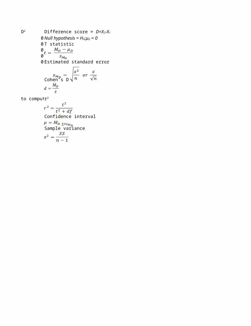
T statistic
Estimated standard error
Cohen's D
Confidence interval
Sample variance
Difference score = D=X2-X1
Null hypothesis = H0:μD = 0
r2
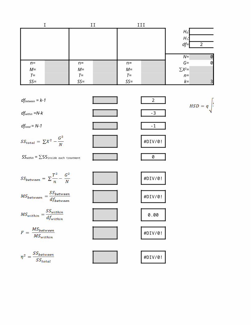
I II III
df= 2 -3 SourceBetween
N= 0 Withinn= n= n= G= 0 TotalM= M= M= ή =T= T= T= n= HSD=SS= SS= SS= k= 3
2
-3
-1
#DIV/0!
0
#DIV/0!
#DIV/0!
0.00
#DIV/0!
#DIV/0!
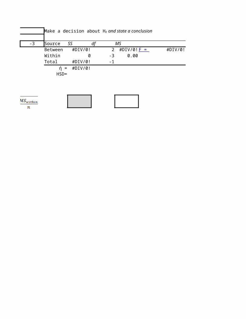
H0: Make a decision about H0 and state a conclusionH1:
∑X2=
dfbetween = k-1
dfwithin =N-k
dftotal = N-1
SSwithin = ∑SSinside each treatment
SS df MS#DIV/0! 2 #DIV/0! #DIV/0!
0 -3 0.00#DIV/0! -1#DIV/0!
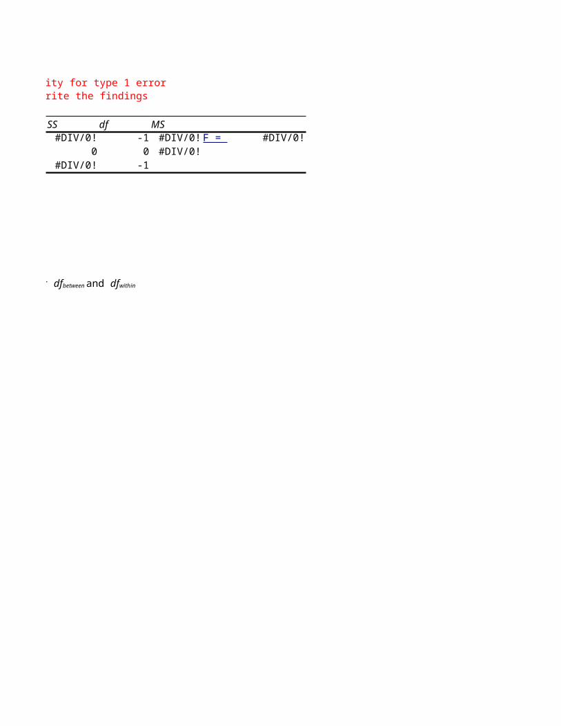
Make a decision about H0 and state a conclusion
F =
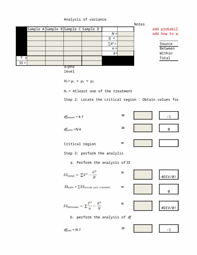
Analysis of varianceNotes
Sample A Sample B Sample C Sample D add probability for type 1 errorN = add how to write the findingsG =
Source SSn = Between #DIV/0!k= Within 0
T = Total #DIV/0!SS =
= -1
= 0
Critical region =
Step 3: perform the analylis
= #DIV/0!
= 0
= #DIV/0!
= -1
∑X2 =
Step 1: State the hypothesis and specify the alpha level
H0 = μ1 = μ2 = μ3
H1 = Atleast one of the treatment means is different
Step 2: Locate the critical region : Obtain values for dfbetween and dfwithin
dfbetween = k-1
dfwithin =N-k
a. Perform the analysis of SS
SSwithin = ∑SSinside each treatment
b. perform the analysis of df
dftotal = N-1
= -1
= 0
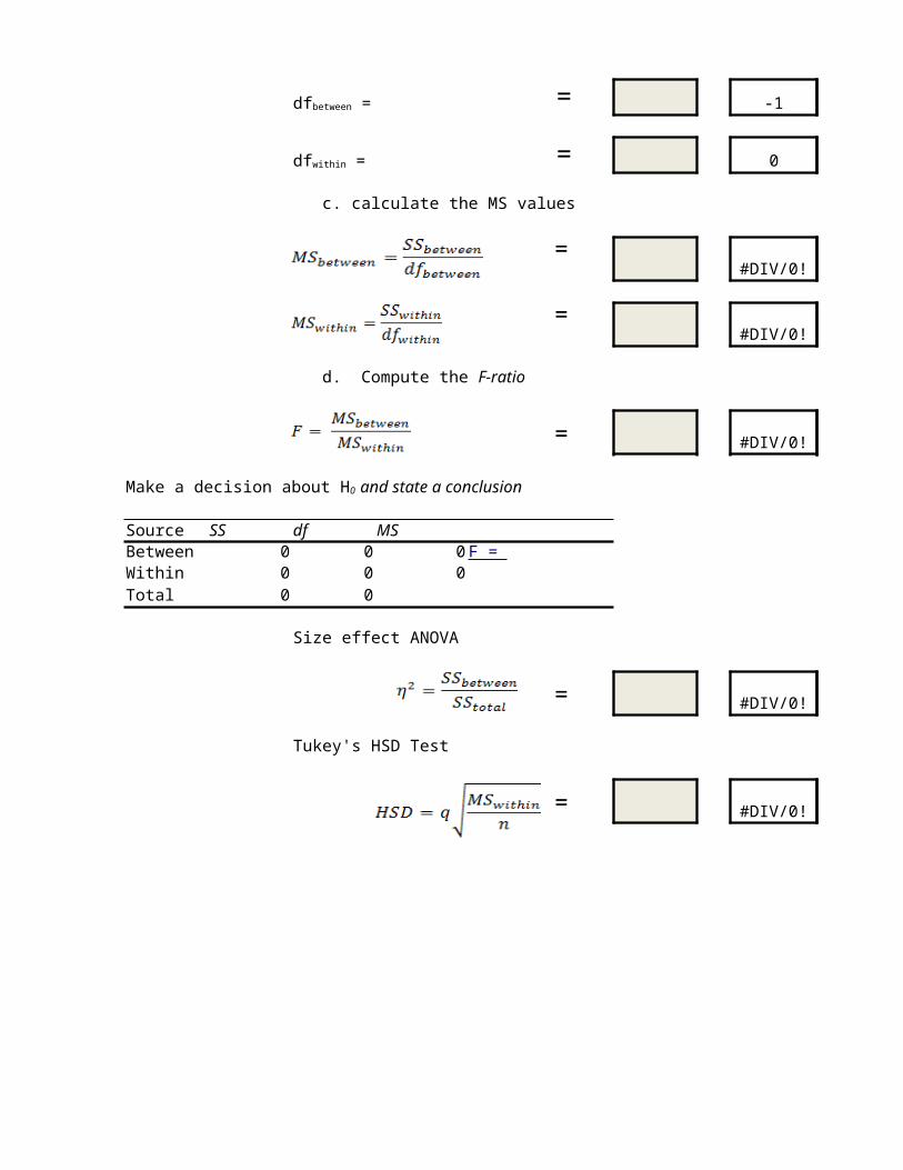
c. calculate the MS values
= #DIV/0!
= #DIV/0!
= #DIV/0!
Source SS df MSBetween 0 0 0 Within 0 0 0Total 0 0
Size effect ANOVA
= #DIV/0!
Tukey's HSD Test
= #DIV/0!
dfbetween =
dfwithin =
d. Compute the F-ratio
Make a decision about H0 and state a conclusion
F =

add probability for type 1 erroradd how to write the findings
df MS-1 #DIV/0! #DIV/0!0 #DIV/0!
-1
F =
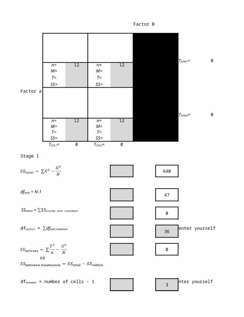
Factor B
0n= 12 n= 12M= M=T= T= N=
Factor aSS= SS= G=
0n= 12 n= 12M= M=T= T=SS= SS=
0 0
Stage 1
640
47
0
36 enter yourself
0
or
3 nter yourself
TROW1=
TROW2=
∑X2=
TCOL1= TCOL2=
dftotal = N-1
SSwithin = ∑SSinside each treatment
dfwithin = ∑dfeach treatment
dfbetween = number of cells - 1
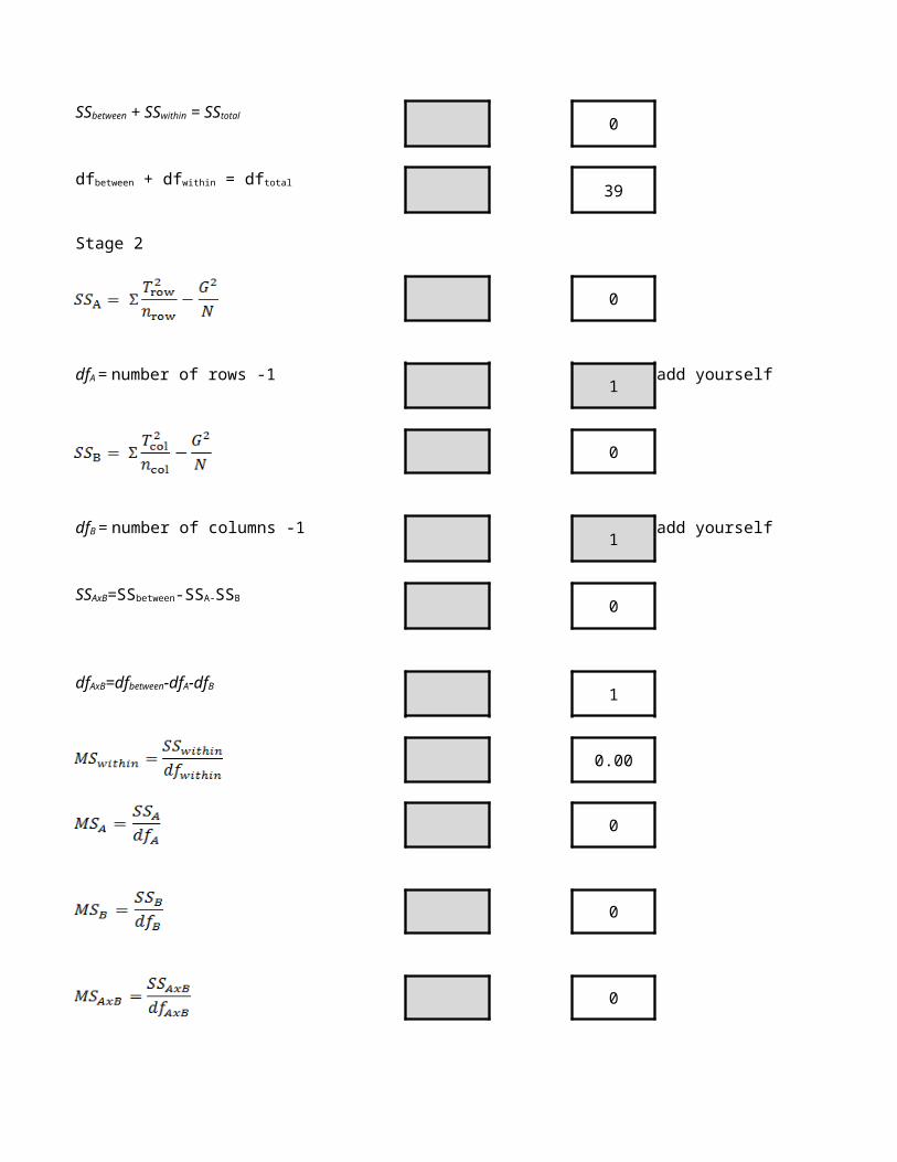
0
39
Stage 2
0
1 add yourself
0
1 add yourself
0
1
0.00
0
0
0
#DIV/0!
SSbetween + SSwithin = SStotal
dfbetween + dfwithin = dftotal
dfA = number of rows -1
dfB = number of columns -1
SSAxB=SSbetween-SSA-SSB
dfAxB=dfbetween-dfA-dfB
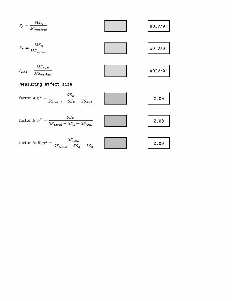
#DIV/0!
#DIV/0!
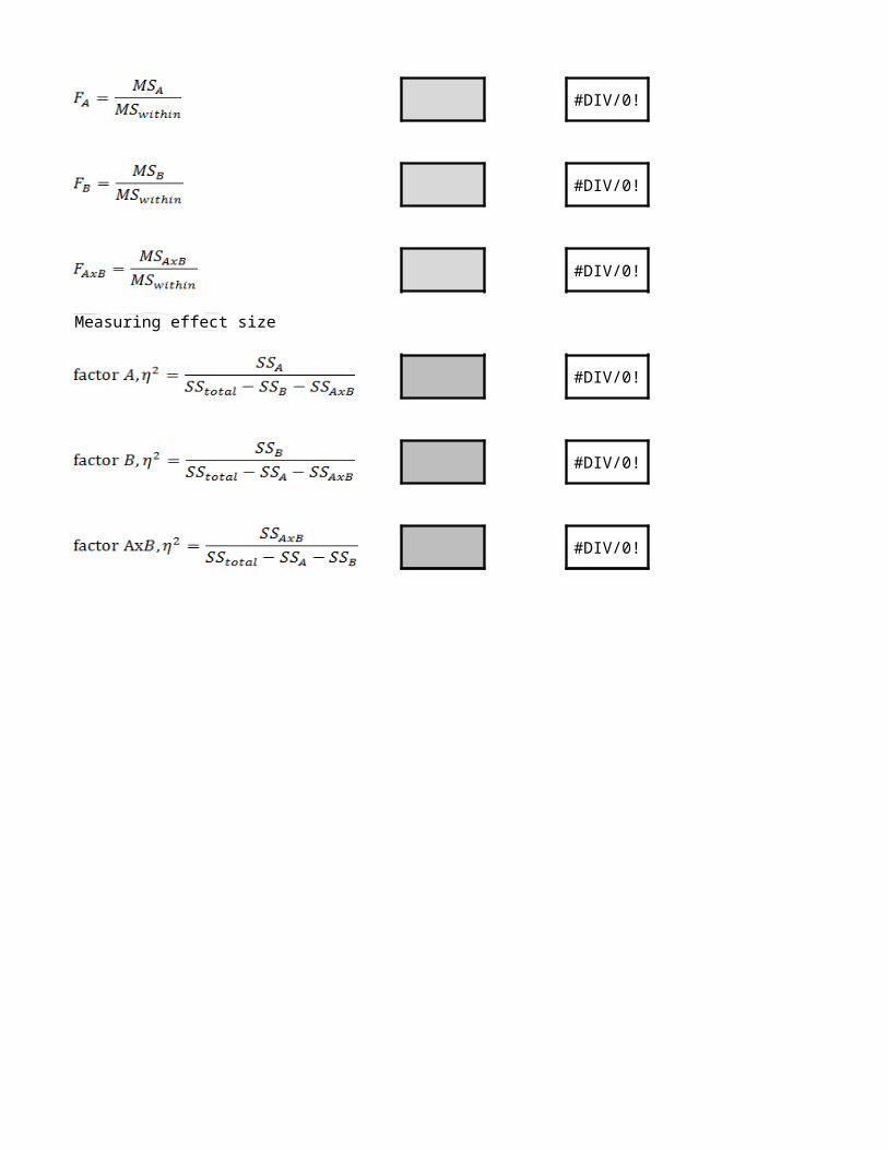
Measuring effect size
0.00
0.00
0.00
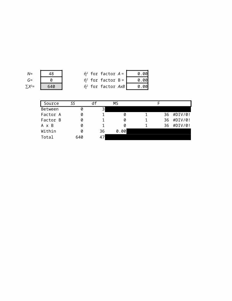
48 0.000 0.00
640 0.00
Source SS df MS FBetween 0 3Factor A 0 1 0 1 36 #DIV/0!Factor B 0 1 0 1 36 #DIV/0!A x B 0 1 0 1 36 #DIV/0!Within 0 36 0.00Total 640 47
ή2 for factor A =ή2 for factor B =ή2 for factor AxB =
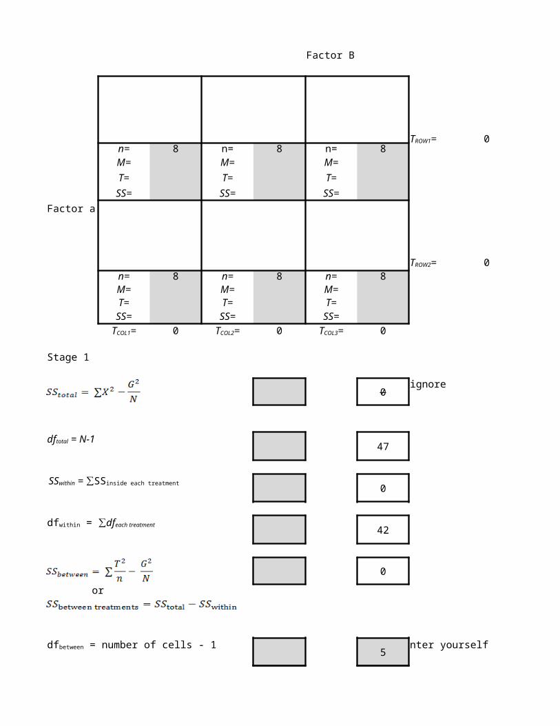
Factor B
0n= 8 n= 8 n= 8M= M= M=T= T= T= N=
Factor aSS= SS= SS= G=
0n= 8 n= 8 n= 8M= M= M=T= T= T=SS= SS= SS=
0 0 0
Stage 1
0ignore
47
0
42
0
or
5 nter yourself
TROW1=
TROW2=
∑X2=
TCOL1= TCOL2= TCOL3=
dftotal = N-1
SSwithin = ∑SSinside each treatment
dfwithin = ∑dfeach treatment
dfbetween = number of cells - 1

0
47
Stage 2
0
1 add yourself
0
2 add yourself
0
2
0.00
0
0
0
#DIV/0!
SSbetween + SSwithin = SStotal
dfbetween + dfwithin = dftotal
dfA = number of rows -1
dfB = number of columns -1
SSAxB=SSbetween-SSA-SSB
dfAxB=dfbetween-dfA-dfB
#DIV/0!
#DIV/0!
Measuring effect size
#DIV/0!
#DIV/0!
#DIV/0!
48 #DIV/0!0 #DIV/0!
#DIV/0!
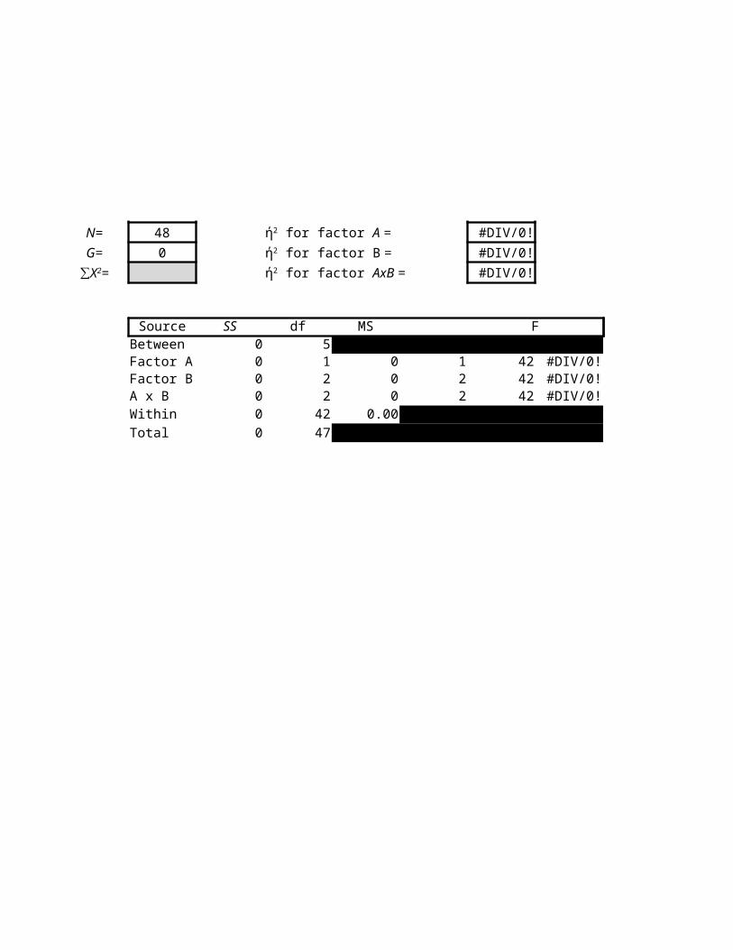
Source SS df MS FBetween 0 5Factor A 0 1 0 1 42 #DIV/0!Factor B 0 2 0 2 42 #DIV/0!A x B 0 2 0 2 42 #DIV/0!Within 0 42 0.00Total 0 47
ή2 for factor A =ή2 for factor B =ή2 for factor AxB =
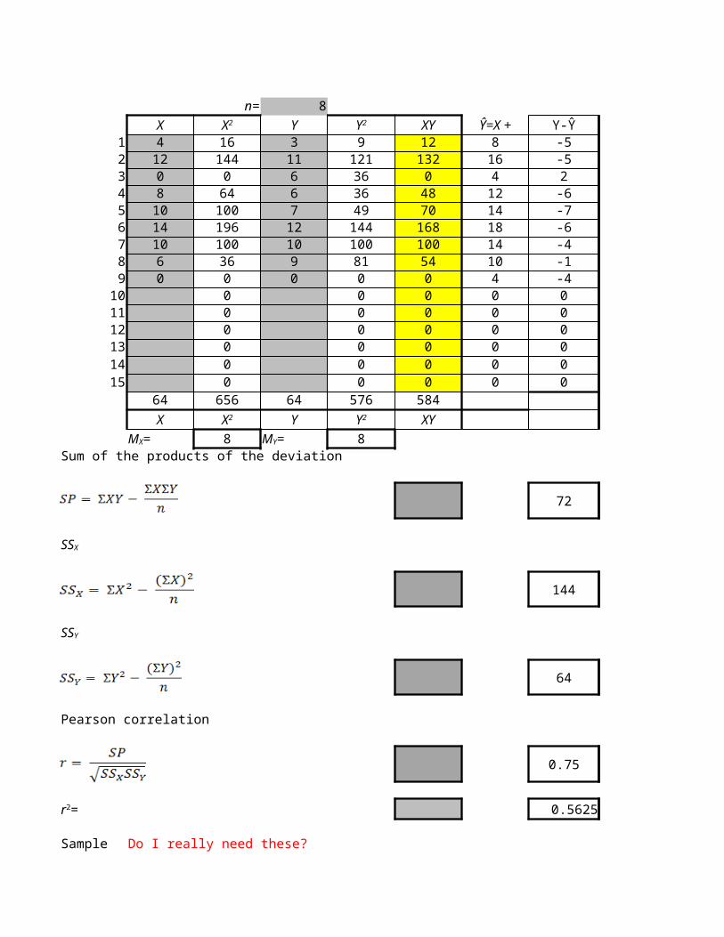
n= 8X Y XY Ŷ=X + Y-Ŷ
1 4 16 3 9 12 8 -5 252 12 144 11 121 132 16 -5 253 0 0 6 36 0 4 2 44 8 64 6 36 48 12 -6 365 10 100 7 49 70 14 -7 496 14 196 12 144 168 18 -6 367 10 100 10 100 100 14 -4 168 6 36 9 81 54 10 -1 19 0 0 0 0 0 4 -4 16
10 0 0 0 0 0 011 0 0 0 0 0 012 0 0 0 0 0 013 0 0 0 0 0 014 0 0 0 0 0 015 0 0 0 0 0 0
64 656 64 576 584X Y XY
8 8Sum of the products of the deviation
72
144
64
Pearson correlation
0.75
0.5625
Sample Do I really need these?
X2 Y2 (Y-Ŷ)2
X2 Y2
MX= MY=
SSX
SSY
r2=
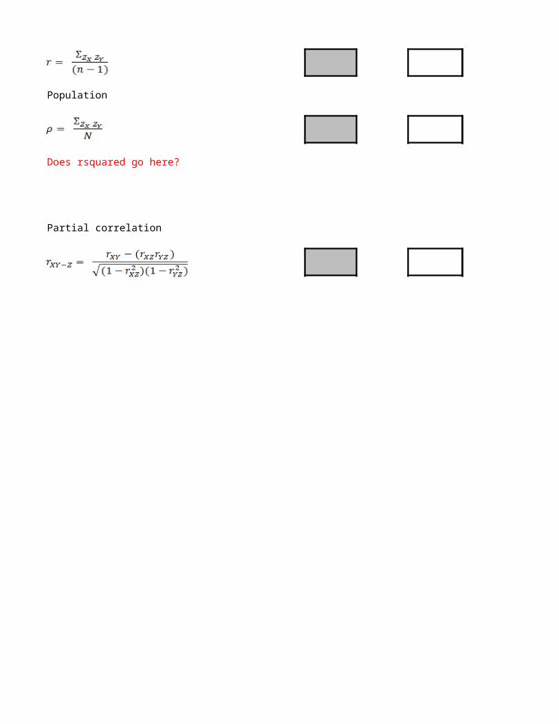
Population
Does rsquared go here?
Partial correlation
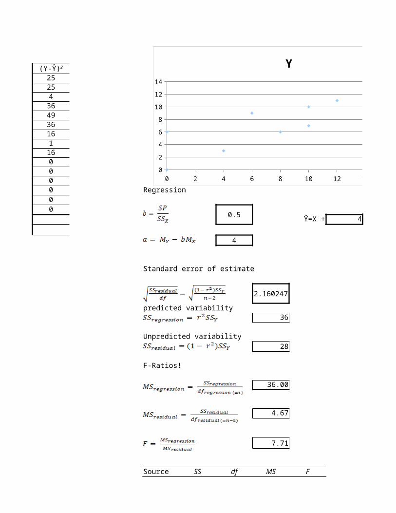
Regression
0.5Ŷ=X + 4
4
Standard error of estimate
2.160247
predicted variability 36
Unpredicted variability28
F-Ratios!
36.00
4.67
7.71
Source SS df MS F
0 2 4 6 8 10 12 14 160
2
4
6
8
10
12
14
Y
Y
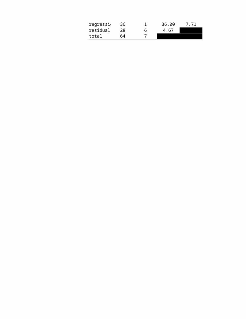
regression 36 1 36.00 7.71residual 28 6 4.67total 64 7

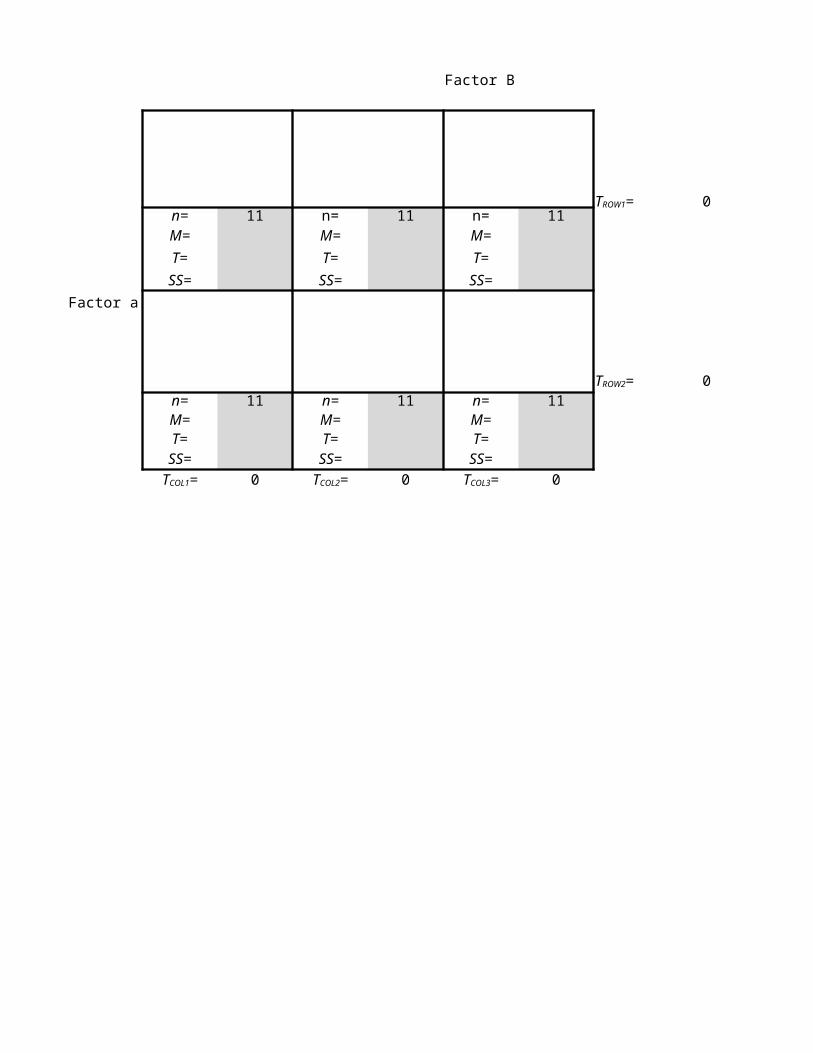
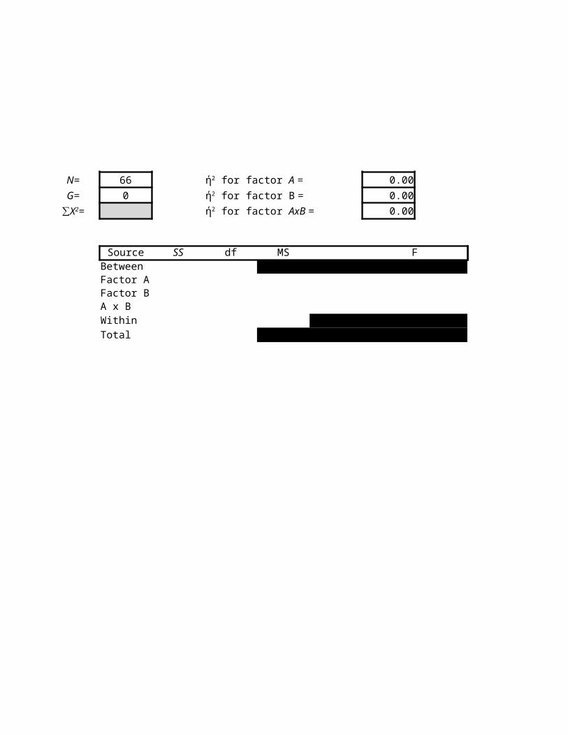
Factor B
0n= 11 n= 11 n= 11M= M= M=T= T= T= N=
Factor aSS= SS= SS= G=
0n= 11 n= 11 n= 11M= M= M=T= T= T=SS= SS= SS=
0 0 0
TROW1=
TROW2=
∑X2=
TCOL1= TCOL2= TCOL3=
66 0.000 0.00
0.00
Source SS df MS FBetweenFactor AFactor BA x BWithinTotal
ή2 for factor A =ή2 for factor B =ή2 for factor AxB =
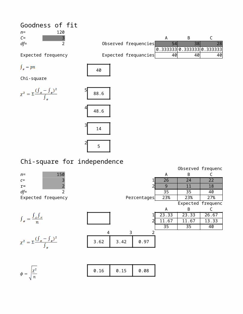
Goodness of fitn= 120C= 3 A B C Ddf= 2 Observed frequencies 54 38 28 0
0.333333 0.333333 0.333333 0.333333Expected frequency Expected frequancies 40 40 40 40
40
Chi-square
588.6
448.6
314
25
Chi-square for independenceObserved frequencies
n= 150 A B C Dc= 3 1 26 24 22 28r= 2 2 9 11 18 12df= 2 35 35 40 40Expected frequency Percentages 23% 23% 27% 27%
Expected frequenciesA B C D
1 23.33 23.33 26.67 26.672 11.67 11.67 13.33 13.33
35 35 40 404 3 2
3.62 3.42 0.97
0.16 0.15 0.08

E0
0.33333340
10050
10050