Stephanie MoyermanMA 164

Final Project04/28/2006

Exploring the Lorenz Equations through a Chaotic Waterwheel

1 Introduction

The Lorenz equations

x = σ(y− x) (1a)y = rx − y− xz (1b)

z = xy− bz (1c)

were derived by Edward Lorenz in 1963 as an over-simplified model of convection rollswithin the atmosphere [1]. These coupled differential equations appear quite harmless;only two terms appear that cause non-linearity. Lorenz found, however, that the behaviorof the system changed drastically over a wide range of parameters. For certain param-eter values, Lorenz discovered that the system exhibited unpredictable and even chaoticbehavior!

Our goal in this paper is to directly explore the properties of the Lorenz equations andtheir exact mechanical analog, a chaotic waterwheel. In subsequent sections, the readerwill encounter the derivation of these amazing equations, an exploration of parameterspace, computational results and trajectories, and an in-depth look at chaos.

2 Derivation

We will derive the Lorenz equations by first deriving the equations of motion for a chaoticwaterwheel and then performing a change of variables.

A schematic diagram of a chaotic waterwheel is given in Figure 1 on the next page.The wheel rests atop a flat surface and is tilted slightly from the horizontal. Water ispumped into the system through a perforated hose at the top and directed into dozens ofsmall nozzles. The nozzles distribute the water at a steady rate into chambers around theside of the wheel. A small hole at the bottom of each chamber allows water to leak out,resulting in a time dependent volume of water in each chamber.

Let us now define our variables and parameters and explain what each entails:

• θ := the angle of rotation in the lab frame

• ω(t) := angular velocity of the wheel, increasing in the counterclockwise direction

1

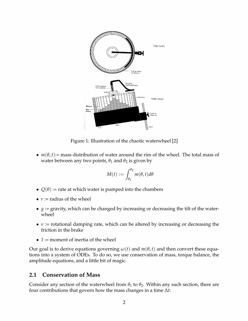
Figure 1: Illustration of the chaotic waterwheel [2]

• m(θ, t):= mass distribution of water around the rim of the wheel. The total mass ofwater between any two points, θ1 and θ2 is given by

M(t) :=∫ θ2

θ1

m(θ, t)dθ

• Q(θ) := rate at which water is pumped into the chambers

• r := radius of the wheel

• g := gravity, which can be changed by increasing or decreasing the tilt of the water-wheel

• ν := rotational damping rate, which can be altered by increasing or decreasing thefriction in the brake

• I := moment of inertia of the wheel

Our goal is to derive equations governing ω(t) and m(θ, t) and then convert these equa-tions into a system of ODEs. To do so, we use conservation of mass, torque balance, theamplitude equations, and a little bit of magic.

2.1 Conservation of Mass

Consider any section of the waterwheel from θ1 to θ2. Within any such section, there arefour contributions that govern how the mass changes in a time ∆t:

2

1. Total mass of inflow water from the pump, given by[ ∫ θ2

θ1Qdθ

].

2. The mass of water that leaks from the system,[−

∫ θ2θ1

Kmdθ]∆t. The factor of m in

the integral is very important. It means that the rate at which water flows out of aregion is proportional to the mass contained within, which matches experimentaldata [2]. It also ensures that water will never flow from a region with no massenclosed.

3. The mass carried in by the rotating wheel. This is given by mθ1ω∆t, where mθ1 isthe mass per unit angle and ω∆t is the angular width.

4. Similarly, the mass that rotates out is −mθ2ω∆t.

Combining these yields

δM = ∆t[ ∫ θ2

θ1

Qdθ −∫ θ2

θ1

Kmdθ]

+ mθ1ω∆t−mθ2ω∆t.

Pulling the rotational terms into the integral, dividing by ∆t and taking the limit as ∆t → 0gives

dMdt

=∫ θ2

θ1

(Q− Km−ω∂m∂θ

)dθ.

Now, exploiting the definition of mass

dMdt

=∫ θ2

θ1

∂m∂t

dθ,

we have ∫ θ2

θ1

∂m∂t

dθ =∫ θ2

θ1

(Q− Km−ω∂m∂θ

)dθ.

As this must hold over any arbitrary interval, the integrands must be equal. This giveswhat is known as our continuity equation:

∂m∂t

= Q− Km−ω∂m∂θ

. (2)

2.2 Torque Balance

To derive our governing equation for ω, we consider the torques applied to the water-wheel. We first note that as t → ∞, the moment of inertia, I, of the wheel tends to aconstant value [2]. Thus we will treat the moment of inertia as a constant in our deriva-tion. This leaves two sources of torque, damping and gravity.

There are two sources of rotational damping in the waterwheel. The first is the brake,which can be adjusted by the user. The second is the introduction of water with ω0 = 0,

3

which must gain momentum until it reaches the system’s velocity ω f = ω. As both offactors are proportional to the angular velocity, we represent this torque as

damping torque = −νω,

where ν > 0.Finally, for an infinitesimal angle dθ, there is a gravitational torque on the system given

by

dτ = mgr sin θdθ.

Here, g = g0 sin α, is the effective gravity, which depends upon the tilt of the waterwheelfrom horizontal, α. Integrating over the total mass and combining with the dampingtorque yields

τ = Iω = −νω + gr∫ 2π

0m(θ, t) sin θdθ, (3)

the equation governing our angular velocity.

2.3 Amplitude Equations

Equations (2) and (3) appear to be a set of very complicated partial, coupled differentialequations. We will now apply the amplitude equations and see the magic happen.

Since the mass is 2π periodic in θ, we may rewrite it as a Fourier series

m(θ, t) =∞

∑n=0

[an(t) sin nθ + bn(t) cos nθ],

where substitution into equations (2) and (3) will yield differential equations for an andbn, known as amplitude equations. We may also write the inflow as a Fourier series

Q(θ) =∞

∑n=0

qn cos nθ,

where the sin term is neglected since the inflow is assumed to be symmetric about θ = 0(the top of the waterwheel).

Substituting our series representations for m and Q into (2) and collecting sin nθ andcos nθ terms gives

an = nωbn − Kanbn = −nωan − Kbn + qn. (4)

We may now recast our equation governing ω in terms of Fourier series as

Iω = −νω + gr∫ 2π

0

[ ∞

∑n=0

an(t) sin nθ + bn(t) cos nθ]

sin θdθ

= −νω + gr∫ 2π

0a1 sin2 θdθ

= −νω + πgra1,

4

where all the other terms have integrated to zero by orthogonality. Thus a1, b1, and ωform a closed system, decoupled from all higher order modes. In fact, for all highermodes, an, bn → 0 as t → ∞. The governing equations for our waterwheel are then

a1 = nωb1 − Ka1 (5a)

b1 = −nωa1 − Kb1 + q1 (5b)ω = (−νω + πgra1)/I. (5c)

2.4 Change of Variables: The Lorenz Equations

Our three dimensional waterwheel system is equivalent to the Lorenz system introducedin equation (1). The change of variables is as follows:

a1 =Kν

πgry

b1 =−Kν

πgrz +

q1

Kω = Kx

t =τ

K,

where the Prandtl number is σ = νKI and the Rayleigh number is r = πgrq1

K2ν. However, note

that with this change of variables, the Lorenz equations parameter b (a parameter thatactually remains nameless) must be set as b = 1, meaning the waterwheel is a specificcase of the broader Lorenz equations. Nonetheless, this simple mechanical system hasbeen transformed into one of the most widely studies chaotic systems known today!

3 Preliminary Analysis of Systems

3.1 The Waterwheel

We begin by exploring the fixed points of equation (5), which are given by:

(a1∗, b1∗, w∗) = (0,q1

K, 0)

(a1∗, b1∗, w∗) = (νω∗πgr

,Kν

πgr,±πgrq1

ν− K2),

where we have left our value of ω∗ in the expression for a1∗ for notational convenience.The first fixed point corresponds to a stationary state. At this fixed point the wheel is

not rotating; inflow is balanced exactly by leakage.The second fixed point corresponds to steady state rotation of the waterwheel in either

direction, dependent upon the sign of ω. Such a solution can exist if and only if

πgrq1

K2ν> 1,

5

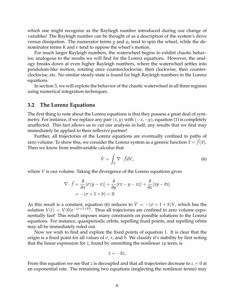
which one might recognize as the Rayliegh number introduced during our change ofvariables! The Rayleigh number can be thought of as a description of the system’s driveversus dissipation. The numerator terms g and q1 tend to spin the wheel, while the de-nominator terms K and ν tend to oppose the wheel’s motion.

For much larger Rayleigh numbers, the waterwheel begins to exhibit chaotic behav-ior, analogous to the results we will find for the Lorenz equations. However, the anal-ogy breaks down at even higher Rayleigh numbers, where the waterwheel settles intopendulum-like motion, rotating once counterclockwise, then clockwise, then counter-clockwise, etc. No similar steady-state is found for high Rayleigh numbers in the Lorenzequations.

In section 3, we will explore the behavior of the chaotic waterwheel in all three regimesusing numerical integration techniques.

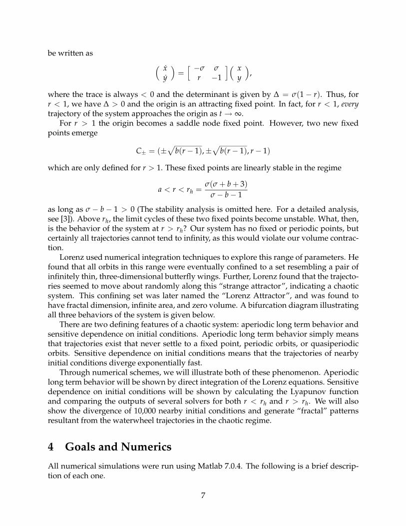
3.2 The Lorenz Equations

The first thing to note about the Lorenz equations is that they possess a great deal of sym-metry. For instance, if we replace any pair (x, y) with (−x,−y), equation (1) is completelyunaffected. This fact allows us to cut our analysis in half; any results that we find mayimmediately be applied to their reflexive partner!

Further, all trajectories of the Lorenz equations are eventually confined to paths ofzero volume. To show this, we consider the Lorenz system as a generic function ~x = ~f (~x).Then we know from multivariable calculus that

V =∫

V∇ · ~f dV, (6)

where V is our volume. Taking the divergence of the Lorenz equations gives

∇ · ~f =∂

∂x[σ(y− x)] +

∂

∂y[rx − y− xz] +

∂

∂z[xy− bz]

= −(σ + 1 + b) < 0.

As this result is a constant, equation (6) reduces to V = −(σ + 1 + b)V, which has thesolution V(t) = V(0)e−(σ+1+b)t. Thus all trajectories are confined to zero volume expo-nentially fast! This result imposes many constraints on possible solutions to the Lorenzequations. For instance, quasiperiodic orbits, repelling fixed points, and repelling orbitsmay all be immediately ruled out.

Now we wish to find and explore the fixed points of equation 1. It is clear that theorigin is a fixed point for all values of σ, r, and b. We classify it’s stability by first notingthat the linear expression for z, found by ommitting the nonlinear xy term, is

z = −bz.

From this equation we see that z is decoupled and that all trajectories decrease to z = 0 atan exponential rate. The remaining two equations (neglecting the nonlinear terms) may

6

be written as ( xy

)=

[ −σ σr −1

]( xy

),

where the trace is always < 0 and the determinant is given by ∆ = σ(1 − r). Thus, forr < 1, we have ∆ > 0 and the origin is an attracting fixed point. In fact, for r < 1, everytrajectory of the system approaches the origin as t → ∞.

For r > 1 the origin becomes a saddle node fixed point. However, two new fixedpoints emerge

C± = (±√

b(r − 1),±√

b(r − 1), r − 1)

which are only defined for r > 1. These fixed points are linearly stable in the regime

a < r < rh =σ(σ + b + 3)

σ− b− 1

as long as σ − b − 1 > 0 (The stability analysis is omitted here. For a detailed analysis,see [3]). Above rh, the limit cycles of these two fixed points become unstable. What, then,is the behavior of the system at r > rh? Our system has no fixed or periodic points, butcertainly all trajectories cannot tend to infinity, as this would violate our volume contrac-tion.

Lorenz used numerical integration techniques to explore this range of parameters. Hefound that all orbits in this range were eventually confined to a set resembling a pair ofinfinitely thin, three-dimensional butterfly wings. Further, Lorenz found that the trajecto-ries seemed to move about randomly along this “strange attractor”, indicating a chaoticsystem. This confining set was later named the “Lorenz Attractor”, and was found tohave fractal dimension, infinite area, and zero volume. A bifurcation diagram illustratingall three behaviors of the system is given below.

There are two defining features of a chaotic system: aperiodic long term behavior andsensitive dependence on initial conditions. Aperiodic long term behavior simply meansthat trajectories exist that never settle to a fixed point, periodic orbits, or quasiperiodicorbits. Sensitive dependence on initial conditions means that the trajectories of nearbyinitial conditions diverge exponentially fast.

Through numerical schemes, we will illustrate both of these phenomenon. Aperiodiclong term behavior will be shown by direct integration of the Lorenz equations. Sensitivedependence on initial conditions will be shown by calculating the Lyapunov functionand comparing the outputs of several solvers for both r < rh and r > rh. We will alsoshow the divergence of 10,000 nearby initial conditions and generate “fractal” patternsresultant from the waterwheel trajectories in the chaotic regime.

4 Goals and Numerics

All numerical simulations were run using Matlab 7.0.4. The following is a brief descrip-tion of each one.

7

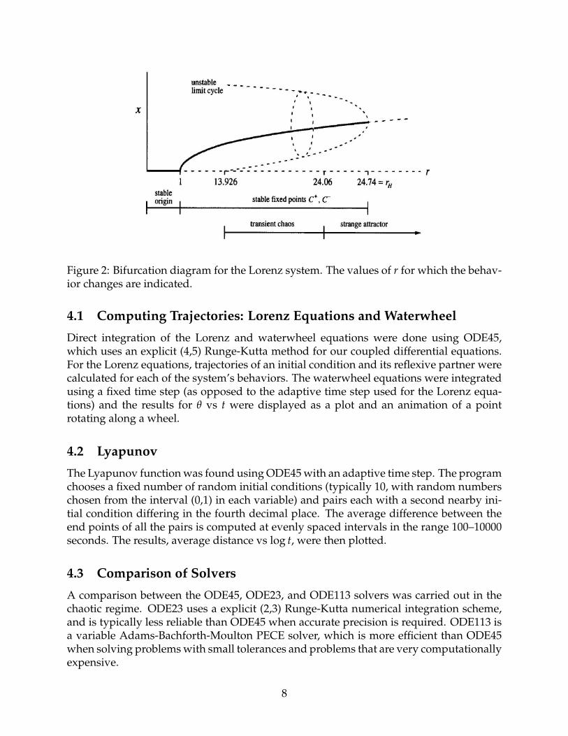
Figure 2: Bifurcation diagram for the Lorenz system. The values of r for which the behav-ior changes are indicated.

4.1 Computing Trajectories: Lorenz Equations and Waterwheel

Direct integration of the Lorenz and waterwheel equations were done using ODE45,which uses an explicit (4,5) Runge-Kutta method for our coupled differential equations.For the Lorenz equations, trajectories of an initial condition and its reflexive partner werecalculated for each of the system’s behaviors. The waterwheel equations were integratedusing a fixed time step (as opposed to the adaptive time step used for the Lorenz equa-tions) and the results for θ vs t were displayed as a plot and an animation of a pointrotating along a wheel.

4.2 Lyapunov

The Lyapunov function was found using ODE45 with an adaptive time step. The programchooses a fixed number of random initial conditions (typically 10, with random numberschosen from the interval (0,1) in each variable) and pairs each with a second nearby ini-tial condition differing in the fourth decimal place. The average difference between theend points of all the pairs is computed at evenly spaced intervals in the range 100–10000seconds. The results, average distance vs log t, were then plotted.

4.3 Comparison of Solvers

A comparison between the ODE45, ODE23, and ODE113 solvers was carried out in thechaotic regime. ODE23 uses a explicit (2,3) Runge-Kutta numerical integration scheme,and is typically less reliable than ODE45 when accurate precision is required. ODE113 isa variable Adams-Bachforth-Moulton PECE solver, which is more efficient than ODE45when solving problems with small tolerances and problems that are very computationallyexpensive.

8

The code itself creates an array of N random starting points (typically 10 points withrandom numbers chosen from the interval (0,1) using a normal distribution), and eval-uates the average final position of these points for each solver at times from 0–60 s inincrements of 1 second. The results of each solver are plotted vs time for comparison.

4.4 Divergence of Trajectories

This program uses ODE45 to solve for the end points of 10,000 nearby (varying in thefourth decimal place) trajectories. All initial conditions begin close to the origin, andtheir final positions at a specified time t are plotted on top of the Lorenz Butterfly forcomparison.

4.5 Fractal Patterns

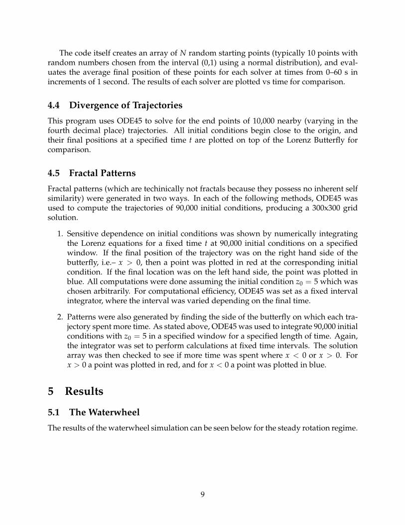
Fractal patterns (which are techinically not fractals because they possess no inherent selfsimilarity) were generated in two ways. In each of the following methods, ODE45 wasused to compute the trajectories of 90,000 initial conditions, producing a 300x300 gridsolution.

1. Sensitive dependence on initial conditions was shown by numerically integratingthe Lorenz equations for a fixed time t at 90,000 initial conditions on a specifiedwindow. If the final position of the trajectory was on the right hand side of thebutterfly, i.e.– x > 0, then a point was plotted in red at the corresponding initialcondition. If the final location was on the left hand side, the point was plotted inblue. All computations were done assuming the initial condition z0 = 5 which waschosen arbitrarily. For computational efficiency, ODE45 was set as a fixed intervalintegrator, where the interval was varied depending on the final time.

2. Patterns were also generated by finding the side of the butterfly on which each tra-jectory spent more time. As stated above, ODE45 was used to integrate 90,000 initialconditions with z0 = 5 in a specified window for a specified length of time. Again,the integrator was set to perform calculations at fixed time intervals. The solutionarray was then checked to see if more time was spent where x < 0 or x > 0. Forx > 0 a point was plotted in red, and for x < 0 a point was plotted in blue.

5 Results

5.1 The Waterwheel

The results of the waterwheel simulation can be seen below for the steady rotation regime.

9

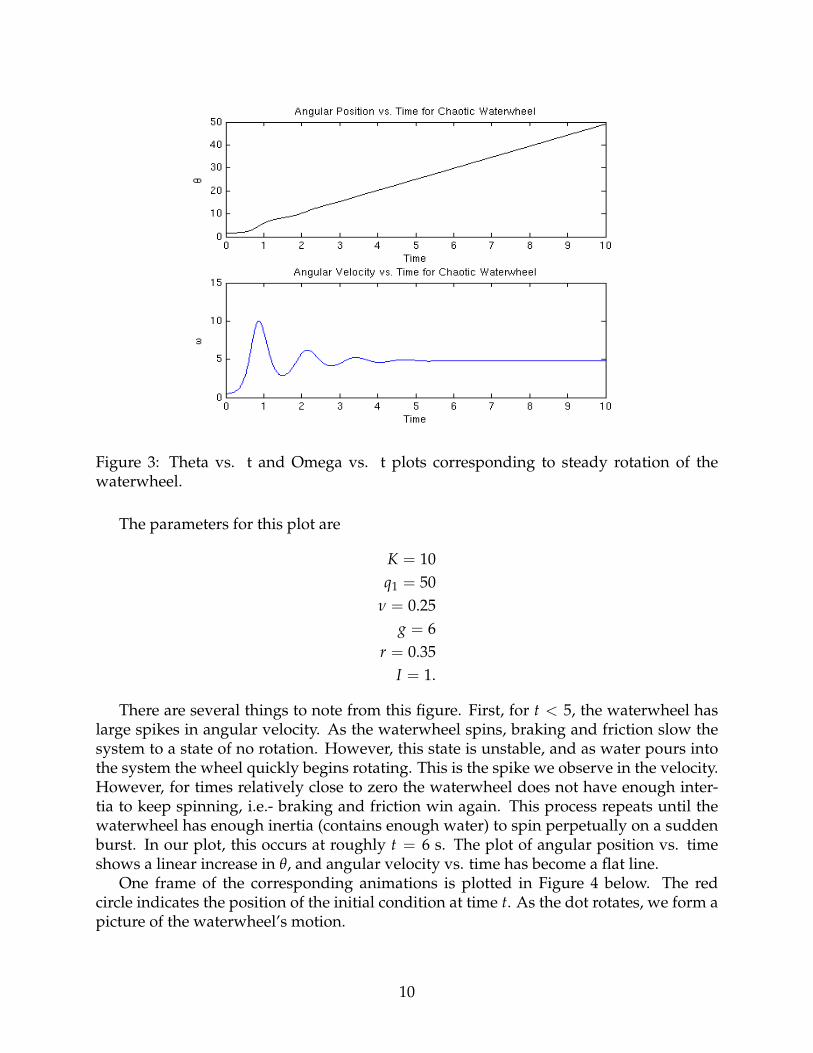
Figure 3: Theta vs. t and Omega vs. t plots corresponding to steady rotation of thewaterwheel.

The parameters for this plot are

K = 10q1 = 50

ν = 0.25g = 6

r = 0.35I = 1.

There are several things to note from this figure. First, for t < 5, the waterwheel haslarge spikes in angular velocity. As the waterwheel spins, braking and friction slow thesystem to a state of no rotation. However, this state is unstable, and as water pours intothe system the wheel quickly begins rotating. This is the spike we observe in the velocity.However, for times relatively close to zero the waterwheel does not have enough inter-tia to keep spinning, i.e.- braking and friction win again. This process repeats until thewaterwheel has enough inertia (contains enough water) to spin perpetually on a suddenburst. In our plot, this occurs at roughly t = 6 s. The plot of angular position vs. timeshows a linear increase in θ, and angular velocity vs. time has become a flat line.

One frame of the corresponding animations is plotted in Figure 4 below. The redcircle indicates the position of the initial condition at time t. As the dot rotates, we form apicture of the waterwheel’s motion.

10

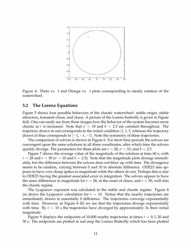
Figure 4: Theta vs. t and Omega vs. t plots corresponding to steady rotation of thewaterwheel.

5.2 The Lorenz Equations

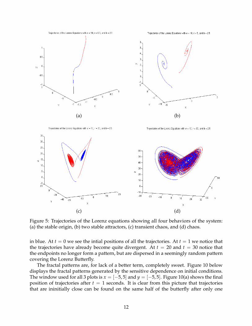
Figure 5 shows four possible behaviors of the chaotic waterwheel: stable origin, stableattractors, transient chaos, and chaos. A picture of the Lorenz butterfly is given in Figure4(d). One can easily see from these images how the behavior of the system becomes morechaotic as r is increased. Note that σ = 10 and b = 2.5 are constant throughout. Thetrajectory drawn in red corresponds to the initial condition [1, 1, 1] whereas the trajectorydrawn in blue corresponds to [−1,−1,−1]. Note the symmetry of these trajectories.

The comparison of solvers is shown in Figure 6. For short time periods the solvers areconvergent upon the same solutions in all three coordinates, after which time the solversquickly diverge. The parameters for these plots are r = 28, σ = 10, and b = 2.5.

Figure 7 shows the average value of the magnitude of the solution at time 60 s, withr = 28 and r = 50 (σ = 10 and b = 2.5). Note that the magnitude plots diverge immedi-ately, but the difference between the solvers does not blow up with time. The divergenceseems to be random, varying between 0 and 10 in absolute difference. ODE23 also ap-pears to have very sharp spikes in magnitude while the others do not. Perhaps this is dueto ODE23 having the greatest associated error in integration. The solvers appear to havethe same differences in magnitude for r = 28, at the onset of chaos, and r = 50, well intothe chaotic regime.

The Lyapunov exponent was calculated in the stable and chaotic regime. Figure 8(a) shows the Lyapunov calculation for r = 10. Notice that the nearby trajectories areimmediately drawn to essentially 0 difference. The trajectories converge exponentiallywith time. However, in Figure 8 (b) we see that the trajectories diverge exponentiallywith time. By t = 10 s the trajectories have diverged by approximately 3x their initialmagnitude.

Figure 9 displays the endpoints of 10,000 nearby trajectories at times t = 0, 1, 20 and30 s. The endpoints are plotted in red atop the Lorenz Butterfly which has been plotted

11

(a) (b)

(c) (d)

Figure 5: Trajectories of the Lorenz equations showing all four behaviors of the system:(a) the stable origin, (b) two stable attractors, (c) transient chaos, and (d) chaos.

in blue. At t = 0 we see the intial positions of all the trajectories. At t = 1 we notice thatthe trajectories have already become quite divergent. At t = 20 and t = 30 notice thatthe endpoints no longer form a pattern, but are dispersed in a seemingly random patterncovering the Lorenz Butterfly.

The fractal patterns are, for lack of a better term, completely sweet. Figure 10 belowdisplays the fractal patterns generated by the sensitive dependence on initial conditions.The window used for all 3 plots is x = [−5, 5] and y = [−5, 5]. Figure 10(a) shows the finalposition of trajectories after t = 1 seconds. It is clear from this picture that trajectoriesthat are ininitially close can be found on the same half of the butterfly after only one

12

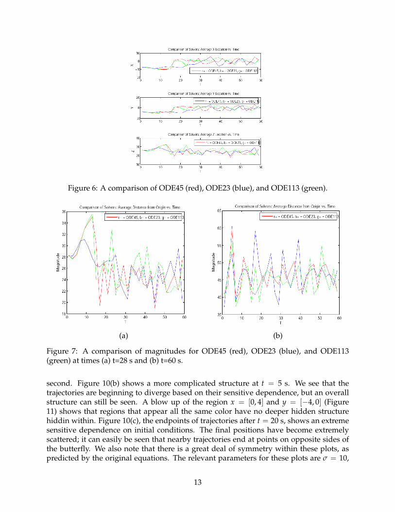
Figure 6: A comparison of ODE45 (red), ODE23 (blue), and ODE113 (green).

(a) (b)

Figure 7: A comparison of magnitudes for ODE45 (red), ODE23 (blue), and ODE113(green) at times (a) t=28 s and (b) t=60 s.

second. Figure 10(b) shows a more complicated structure at t = 5 s. We see that thetrajectories are beginning to diverge based on their sensitive dependence, but an overallstructure can still be seen. A blow up of the region x = [0, 4] and y = [−4, 0] (Figure11) shows that regions that appear all the same color have no deeper hidden structurehiddin within. Figure 10(c), the endpoints of trajectories after t = 20 s, shows an extremesensitive dependence on initial conditions. The final positions have become extremelyscattered; it can easily be seen that nearby trajectories end at points on opposite sides ofthe butterfly. We also note that there is a great deal of symmetry within these plots, aspredicted by the original equations. The relevant parameters for these plots are σ = 10,

13

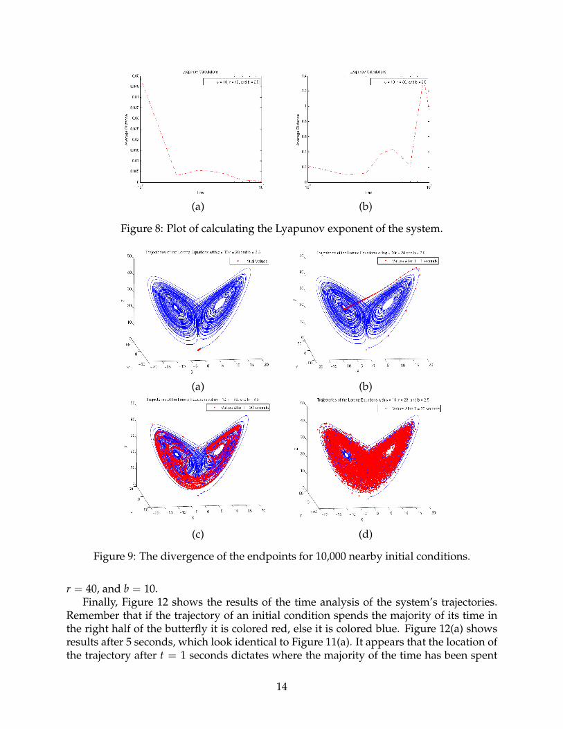
(a) (b)

Figure 8: Plot of calculating the Lyapunov exponent of the system.

(a) (b)

(c) (d)

Figure 9: The divergence of the endpoints for 10,000 nearby initial conditions.

r = 40, and b = 10.Finally, Figure 12 shows the results of the time analysis of the system’s trajectories.

Remember that if the trajectory of an initial condition spends the majority of its time inthe right half of the butterfly it is colored red, else it is colored blue. Figure 12(a) showsresults after 5 seconds, which look identical to Figure 11(a). It appears that the location ofthe trajectory after t = 1 seconds dictates where the majority of the time has been spent

14

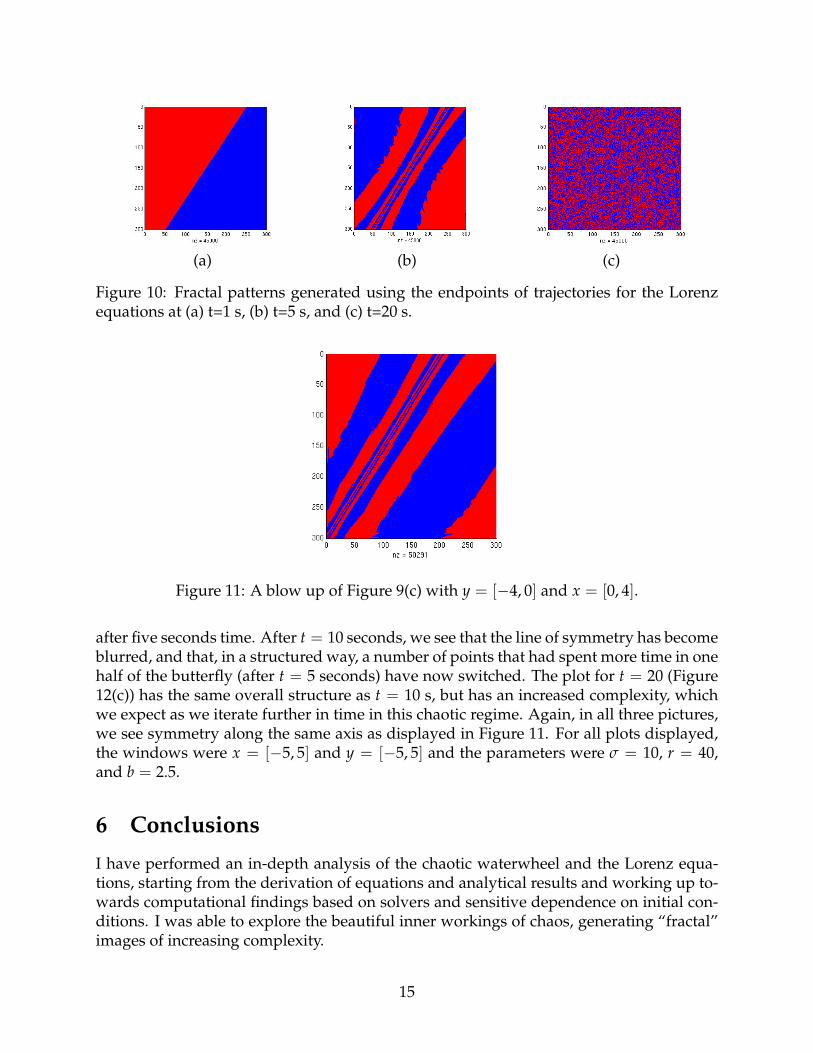
(a) (b) (c)

Figure 10: Fractal patterns generated using the endpoints of trajectories for the Lorenzequations at (a) t=1 s, (b) t=5 s, and (c) t=20 s.

Figure 11: A blow up of Figure 9(c) with y = [−4, 0] and x = [0, 4].

after five seconds time. After t = 10 seconds, we see that the line of symmetry has becomeblurred, and that, in a structured way, a number of points that had spent more time in onehalf of the butterfly (after t = 5 seconds) have now switched. The plot for t = 20 (Figure12(c)) has the same overall structure as t = 10 s, but has an increased complexity, whichwe expect as we iterate further in time in this chaotic regime. Again, in all three pictures,we see symmetry along the same axis as displayed in Figure 11. For all plots displayed,the windows were x = [−5, 5] and y = [−5, 5] and the parameters were σ = 10, r = 40,and b = 2.5.

6 Conclusions

I have performed an in-depth analysis of the chaotic waterwheel and the Lorenz equa-tions, starting from the derivation of equations and analytical results and working up to-wards computational findings based on solvers and sensitive dependence on initial con-ditions. I was able to explore the beautiful inner workings of chaos, generating “fractal”images of increasing complexity.

15

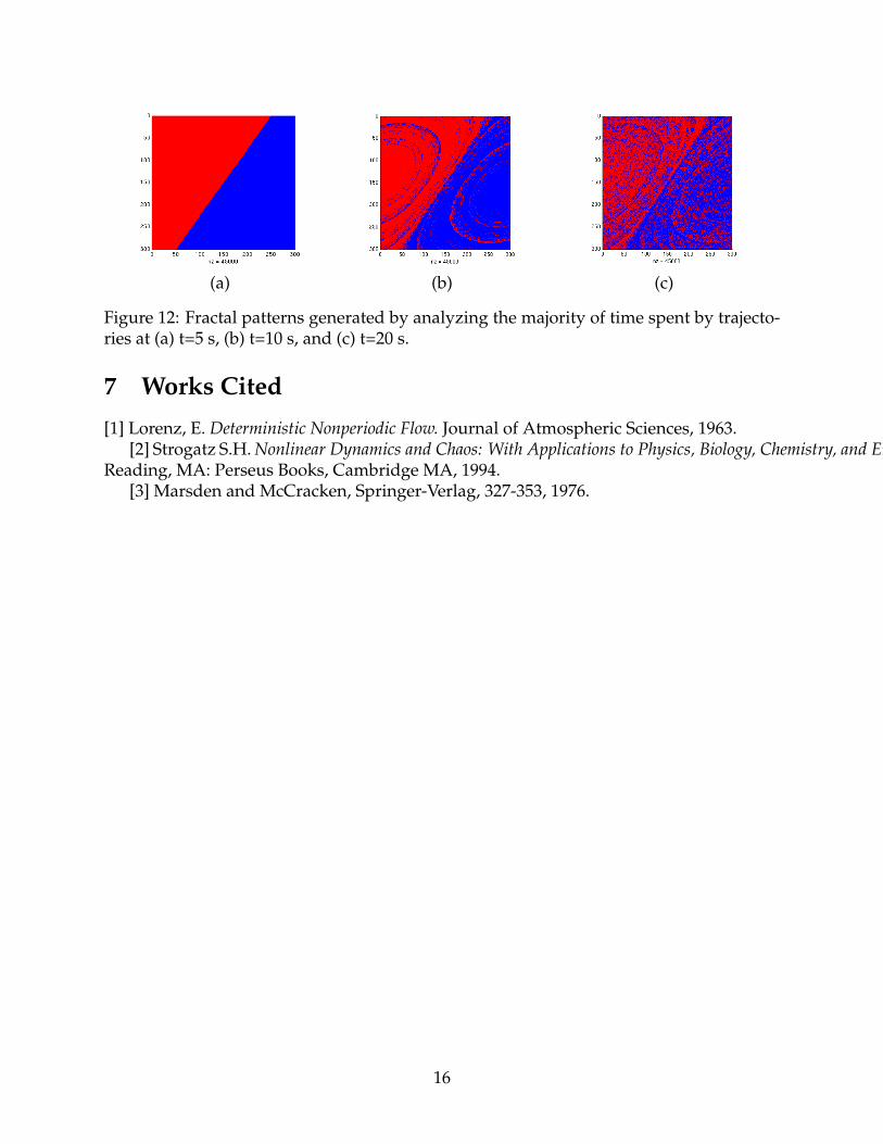
(a) (b) (c)

Figure 12: Fractal patterns generated by analyzing the majority of time spent by trajecto-ries at (a) t=5 s, (b) t=10 s, and (c) t=20 s.

7 Works Cited

[1] Lorenz, E. Deterministic Nonperiodic Flow. Journal of Atmospheric Sciences, 1963.[2] Strogatz S.H. Nonlinear Dynamics and Chaos: With Applications to Physics, Biology, Chemistry, and Engineering.

Reading, MA: Perseus Books, Cambridge MA, 1994.[3] Marsden and McCracken, Springer-Verlag, 327-353, 1976.

16