Coupled Oscillators - Harvey Mudd...

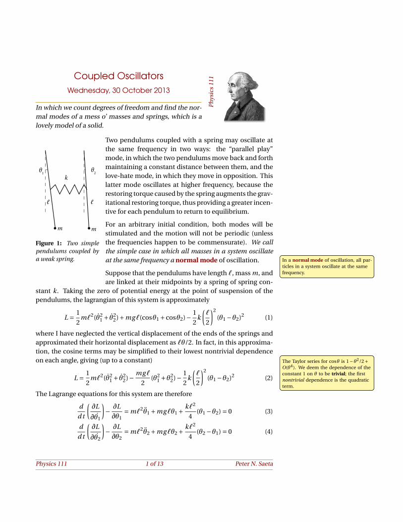
Coupled OscillatorsWednesday, 30 October 2013

In which we count degrees of freedom and find the nor-mal modes of a mess o’ masses and springs, which is alovely model of a solid.

Ph

ysic

s11

1

m

θ2θ1k

ℓℓ

m

Figure 1: Two simplependulums coupled bya weak spring.

Two pendulums coupled with a spring may oscillate atthe same frequency in two ways: the “parallel play”mode, in which the two pendulums move back and forthmaintaining a constant distance between them, and thelove-hate mode, in which they move in opposition. Thislatter mode oscillates at higher frequency, because therestoring torque caused by the spring augments the grav-itational restoring torque, thus providing a greater incen-tive for each pendulum to return to equilibrium.

For an arbitrary initial condition, both modes will bestimulated and the motion will not be periodic (unlessthe frequencies happen to be commensurate). We callthe simple case in which all masses in a system oscillateat the same frequency a normal mode of oscillation. In a normal mode of oscillation, all par-

ticles in a system oscillate at the samefrequency.

In a normal mode of oscillation, all par-ticles in a system oscillate at the samefrequency.Suppose that the pendulums have length `, mass m, and

are linked at their midpoints by a spring of spring con-stant k. Taking the zero of potential energy at the point of suspension of thependulums, the lagrangian of this system is approximately

L = 1

2m`2(θ2

1 + θ22)+mg`(cosθ1 +cosθ2)− 1

2k

(`

2

)2

(θ1 −θ2)2 (1)

where I have neglected the vertical displacement of the ends of the springs andapproximated their horizontal displacement as `θ/2. In fact, in this approxima-tion, the cosine terms may be simplified to their lowest nontrivial dependenceon each angle, giving (up to a constant) The Taylor series for cosθ is 1−θ2/2+

O(θ4). We deem the dependence of theconstant 1 on θ to be trivial; the firstnontrivial dependence is the quadraticterm.

The Taylor series for cosθ is 1−θ2/2+O(θ4). We deem the dependence of theconstant 1 on θ to be trivial; the firstnontrivial dependence is the quadraticterm.

L = 1

2m`2(θ2

1 + θ22)− mg`

2(θ2

1 +θ22)− 1

2k

(`

2

)2

(θ1 −θ2)2 (2)

The Lagrange equations for this system are therefore

d

d t

(∂L

∂θ1

)− ∂L

∂θ1= m`2θ1 +mg`θ1 + k`2

4(θ1 −θ2) = 0 (3)

d

d t

(∂L

∂θ2

)− ∂L

∂θ2= m`2θ2 +mg`θ2 + k`2

4(θ2 −θ1) = 0 (4)

Physics 111 1 of 13 Peter N. Saeta

Divide these equations by m`2 to tidy them up a bit:

θ1 + g

`θ1 + k

4m(θ1 −θ2) = 0 (5)

θ2 + g

`θ2 + k

4m(θ2 −θ1) = 0 (6)

What happens to these equations if θ1(t ) = θ2(t )? Then the coupling terms dis-appear and we are left with identical simple harmonic oscillator equations. So,we deduce that one solution is of the form

θ1 = θ2 = c1 cos(ω0t +φ1) = d1 cosω0t +d2 sinω0t (7)

where ω20 = g /`, and c1 and φ1 (or equivalently d1 and d2) are constants to be

determined by initial conditions.

A second solution may be found by assuming that θ1 =−θ2. Then the first equa-tion becomes

θ1 + g

`θ1 + k

2mθ1 = 0

which is also the simple harmonic oscillator equation, with solution

θ1 =−θ2 = c2 cos(ω1t +φ2) (8)

where ω1 =√

g` + k

2m , and c2 and φ2 are constants.

The two boxed equations are the two normal modes of the coupled pendulumsystem. In a normal mode, all the particles oscillate at the same frequency (butnot necessarily the same amplitude or phase). An arbitrary motion of the un-forced system is a linear combination (superposition) of the two normal modes,with amplitudes and phases chosen to match the given initial conditions.

Example 1 At t = 0 we thump the first mass. What is the subsequent motion?

We’ll assume that the thump takes place over negligible time, and servesto launch m1 at some initial angular velocity θ1(0) =Ω. If the first normalmode is described by d1 cosω0t+d2 sinω0t , while the second is described


by d3 cosω1t +d4 sinω1t , then

θ1(0) = d1 +d3 θ1(0) = d2ω0 +d4ω1 =Ωθ2(0) = d1 −d3 θ2(0) = d2ω0 −d4ω1 = 0

The angular positions require that d1 = d3 = 0, while the angular velocitiesrequire that d2ω0 = d4ω1 =Ω/2. Therefore,

θ1(t ) = Ω

2ω0sinω0t + Ω

2ω1sinω1t (9)

θ2(t ) = Ω

2ω0sinω0t − Ω

2ω1sinω1t (10)

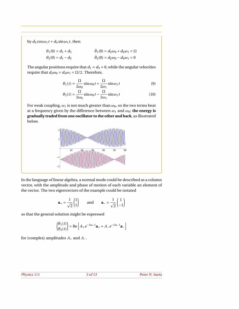
For weak coupling, ω1 is not much greater than ω0, so the two terms beatat a frequency given by the difference between ω1 and ω0; the energy isgradually traded from one oscillator to the other and back, as illustratedbelow.

10 20 30 40 50 60

-2

-1

1

2

In the language of linear algebra, a normal mode could be described as a columnvector, with the amplitude and phase of motion of each variable an element ofthe vector. The two eigenvectors of the example could be notated

a+ = 1p2

(11

)and a− = 1p

2

(1−1

)so that the general solution might be expressed(

θ1(t )θ2(t )

)= Re

[A+e−iω+t a++ A−e−iω−t a−

]for (complex) amplitudes A+ and A−.


1. GENERALIZATION TO N COUPLED PARTICLES

1. Generalization to N Coupled Particles

We now wish to generalize this example to a system of N masses coupled withvarious springs to form a molecule or solid with a stable equilibrium configura-tion. On perturbing one or more of the masses from equilibrium, what sort ofmotion arises?

The motion is bound to be complicated, with each mass ending up coupled toevery other one via the intermediary of one or more springs. It seems reason-able that even if all masses were initially at rest, they will all end up moving insome complicated fashion. The amazing result, however, is that we can al-ways decompose the motion into a linear combination of vibrations in nor-mal modes, with each particle vibrating at the same frequency. Typically, thenormal modes oscillate at different frequencies, however, so their superpositionproduces a motion significantly more complicated than sinusoidal. The motionwithin each normal mode takes place independent of that in every other; eachnormal mode vibration is described with a single amplitude and phase. Hence,the complete behavior is specified by determining the amplitude and phase ofvibration in each of the normal modes.

If the system is three-dimensional, we will need 3N generalized coordinates q j

( j = 1, 2, . . . , 3N ) to describe the configuration of the system, and a correspond-ing number of generalized velocities q j . Of the 3N degrees of freedom, 3 corre-spond to the center of mass translation of the system, and 3 to its rotation (un-less the system happens to be a linear molecule, in which case the molecule canrotate only about two axes). None of these coordinates has a restoring force; ab-sent external influences, their momenta will be constants of the motion. I thinkthat it’s easiest to think of these modes as a special sort of normal mode withvanishing frequency. We will consider rigid-body rotations

and center-of-mass translations as nor-mal modes of vanishing frequency.

We will consider rigid-body rotationsand center-of-mass translations as nor-mal modes of vanishing frequency.This leaves 3N − 6 degrees of freedom associated with distortions away from

equilibrium positions (except for linear molecules, in which case there are 3N−5remaining degrees of freedom associated with normal modes of nonzero fre-quency). We will show that each of these gives rise to a normal mode of vibra-tion, in which all the masses oscillate at the same (nonzero) frequency. Further-more, each normal mode is independent of all the others, so that the 3N − 6coupled oscillators factor into 3N −6 decoupled (independent) oscillators. In the limit we consider, where the po-

tential is strictly a quadratic function ofthe coordinates, each normal mode isindependent of every other one, and thefull motion is a linear superposition ofthe motion of each normal mode.

In the limit we consider, where the po-tential is strictly a quadratic function ofthe coordinates, each normal mode isindependent of every other one, and thefull motion is a linear superposition ofthe motion of each normal mode.

We will work in the center of mass frame and disregard rigid-body rotation. Thenin the equilibrium configuration,

q j = q j 0, q j = 0, q j = 0, j = 1,2, . . . ,n

where n = 3N −6 (or 3N −5 if linear). Lagrange’s equation for the j th coordinate



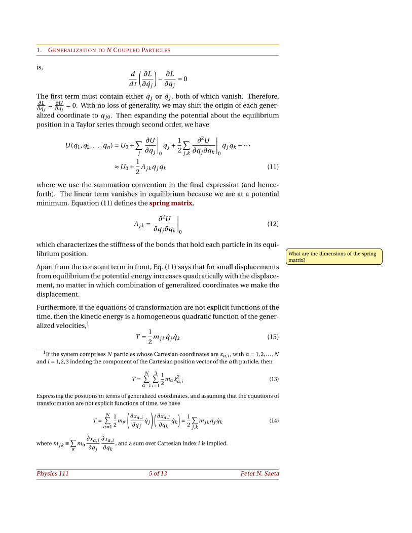
is,d

d t

(∂L

∂q j

)− ∂L

∂q j= 0

The first term must contain either q j or q j , both of which vanish. Therefore,∂L∂q j

= ∂U∂q j

= 0. With no loss of generality, we may shift the origin of each gener-

alized coordinate to q j 0. Then expanding the potential about the equilibriumposition in a Taylor series through second order, we have

U (q1, q2, . . . , qn) =U0 +∑

j

∂U

∂q j

∣∣∣∣0

q j + 1

2

∑j ,k

∂2U

∂q j∂qk

∣∣∣∣0

q j qk +·· ·

≈U0 + 1

2A j k q j qk (11)

where we use the summation convention in the final expression (and hence-forth). The linear term vanishes in equilibrium because we are at a potentialminimum. Equation (11) defines the spring matrix,

A j k = ∂2U

∂q j∂qk

∣∣∣∣0

(12)

which characterizes the stiffness of the bonds that hold each particle in its equi-librium position. What are the dimensions of the spring

matrix?What are the dimensions of the springmatrix?

Apart from the constant term in front, Eq. (11) says that for small displacementsfrom equilibrium the potential energy increases quadratically with the displace-ment, no matter in which combination of generalized coordinates we make thedisplacement.

Furthermore, if the equations of transformation are not explicit functions of thetime, then the kinetic energy is a homogeneous quadratic function of the gener-alized velocities,1

T = 1

2m j k q j qk (15)

1If the system comprises N particles whose Cartesian coordinates are xα,i , with α = 1,2, . . . , Nand i = 1,2,3 indexing the component of the Cartesian position vector of the αth particle, then

T =N∑α=1

3∑i=1

1

2mα x2

α,i (13)

Expressing the positions in terms of generalized coordinates, and assuming that the equations oftransformation are not explicit functions of time, we have

T =N∑α=1

1

2mα

(∂xα,i

∂q jq j

)(∂xα,i

∂qkqk

)= 1

2

∑j ,k

m j k q j qk (14)

where m j k ≡∑α

mα∂xα,i

∂q j

∂xα,i

∂qk, and a sum over Cartesian index i is implied.



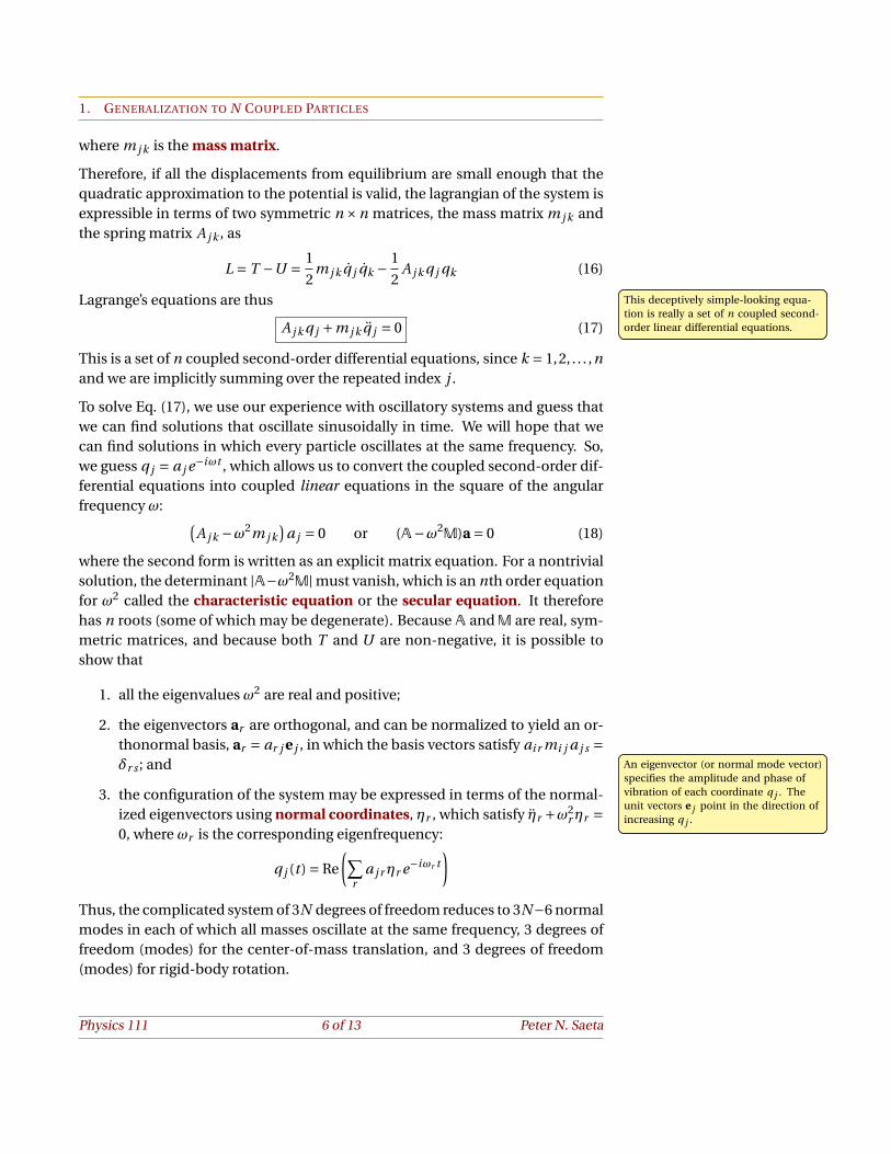
where m j k is the mass matrix.

Therefore, if all the displacements from equilibrium are small enough that thequadratic approximation to the potential is valid, the lagrangian of the system isexpressible in terms of two symmetric n ×n matrices, the mass matrix m j k andthe spring matrix A j k , as

L = T −U = 1

2m j k q j qk −

1

2A j k q j qk (16)

Lagrange’s equations are thus This deceptively simple-looking equa-tion is really a set of n coupled second-order linear differential equations.

This deceptively simple-looking equa-tion is really a set of n coupled second-order linear differential equations.A j k q j +m j k q j = 0 (17)

This is a set of n coupled second-order differential equations, since k = 1,2, . . . ,nand we are implicitly summing over the repeated index j .

To solve Eq. (17), we use our experience with oscillatory systems and guess thatwe can find solutions that oscillate sinusoidally in time. We will hope that wecan find solutions in which every particle oscillates at the same frequency. So,we guess q j = a j e−iωt , which allows us to convert the coupled second-order dif-ferential equations into coupled linear equations in the square of the angularfrequency ω: (

A j k −ω2m j k)

a j = 0 or (A−ω2M)a = 0 (18)

where the second form is written as an explicit matrix equation. For a nontrivialsolution, the determinant |A−ω2M| must vanish, which is an nth order equationfor ω2 called the characteristic equation or the secular equation. It thereforehas n roots (some of which may be degenerate). BecauseA andM are real, sym-metric matrices, and because both T and U are non-negative, it is possible toshow that

1. all the eigenvalues ω2 are real and positive;

2. the eigenvectors ar are orthogonal, and can be normalized to yield an or-thonormal basis, ar = ar j e j , in which the basis vectors satisfy ai r mi j a j s =δr s ; and An eigenvector (or normal mode vector)

specifies the amplitude and phase ofvibration of each coordinate q j . Theunit vectors e j point in the direction ofincreasing q j .

An eigenvector (or normal mode vector)specifies the amplitude and phase ofvibration of each coordinate q j . Theunit vectors e j point in the direction ofincreasing q j .

3. the configuration of the system may be expressed in terms of the normal-ized eigenvectors using normal coordinates, ηr , which satisfy ηr +ω2

rηr =0, where ωr is the corresponding eigenfrequency:

q j (t ) = Re

(∑r

a j rηr e−iωr t)

Thus, the complicated system of 3N degrees of freedom reduces to 3N−6 normalmodes in each of which all masses oscillate at the same frequency, 3 degrees offreedom (modes) for the center-of-mass translation, and 3 degrees of freedom(modes) for rigid-body rotation.


2. LINEAR ALGEBRA

2. Linear Algebra

Perhaps you are so familiar with linear algebra that the above consequences areobvious. If so, you had a much better course than I did (which, frankly, isn’tsaying much!). You can skip to the example.

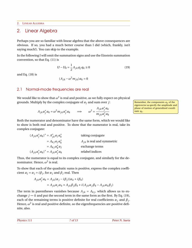
In the following I will omit the summation signs and use the Einstein summationconvention, so that Eq. (11) is

U −U0 = 1

2A j k q j qk ≥ 0 (19)

and Eq. (18) is(A j k −ω2m j k )ak = 0

2.1 Normal-mode frequencies are real

We would like to show that ω2 is real and positive, as we fully expect on physicalgrounds. Multiply by the complex conjugate of a j and sum over j : Remember, the components ak of the

eigenvector a specify the amplitude andphase of motion of generalized coordi-nate qk .

Remember, the components ak of theeigenvector a specify the amplitude andphase of motion of generalized coordi-nate qk .A j k a∗

j ak =ω2m j k a∗j ak =⇒ ω2 =

A j k a∗j ak

m j k a∗j ak

Both the numerator and denominator have the same form, which we would liketo show is both real and positive. To show that the numerator is real, take itscomplex conjugate:

(A j k a∗j ak )∗ = A∗

j k a j a∗k taking conjugate

= Ak j a j a∗k A j k is real and symmetric

= Ak j a∗k a j exchange terms

(A j k a∗j ak )∗ = A j k a∗

j ak relabel indices

Thus, the numerator is equal to its complex conjugate, and similarly for the de-nominator. Hence, ω2 is real.

To show that each of the quadratic sums is positive, express the complex coeffi-cient a j =α j + iβ j , for α j and β j real. Then

A j k a∗j ak = A j k (α j − iβ j )(αk + iβk )

= A j kα jαk + A j kβ jβk + i (A j kα jβk − A j kαkβ j )

The term in parentheses vanishes because A j k = Ak j , which allows us to ex-change j ↔ k and put the second term in the same form as the first. By Eq. (19),each of the remaining terms is positive definite for real coefficients α j and β j .Hence, ω2 is real and positive definite, so the eigenfrequencies are positive defi-nite, also.


2. LINEAR ALGEBRA 2.2 The Eigenvectors are orthogonal

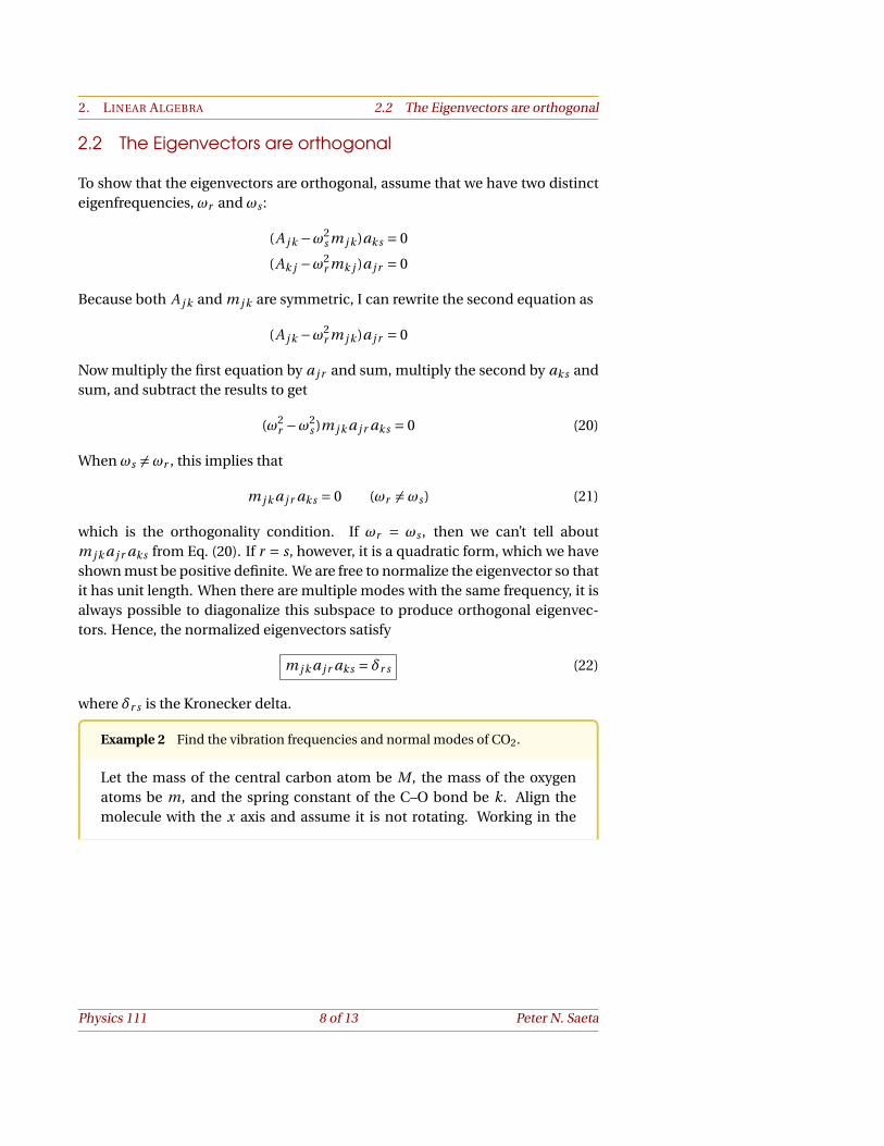
2.2 The Eigenvectors are orthogonal

To show that the eigenvectors are orthogonal, assume that we have two distincteigenfrequencies, ωr and ωs :

(A j k −ω2s m j k )aks = 0

(Ak j −ω2r mk j )a j r = 0

Because both A j k and m j k are symmetric, I can rewrite the second equation as

(A j k −ω2r m j k )a j r = 0

Now multiply the first equation by a j r and sum, multiply the second by aks andsum, and subtract the results to get

(ω2r −ω2

s )m j k a j r aks = 0 (20)

When ωs 6=ωr , this implies that

m j k a j r aks = 0 (ωr 6=ωs) (21)

which is the orthogonality condition. If ωr = ωs , then we can’t tell aboutm j k a j r aks from Eq. (20). If r = s, however, it is a quadratic form, which we haveshown must be positive definite. We are free to normalize the eigenvector so thatit has unit length. When there are multiple modes with the same frequency, it isalways possible to diagonalize this subspace to produce orthogonal eigenvec-tors. Hence, the normalized eigenvectors satisfy

m j k a j r aks = δr s (22)

where δr s is the Kronecker delta.

Example 2 Find the vibration frequencies and normal modes of CO2.

Let the mass of the central carbon atom be M , the mass of the oxygenatoms be m, and the spring constant of the C–O bond be k. Align themolecule with the x axis and assume it is not rotating. Working in the



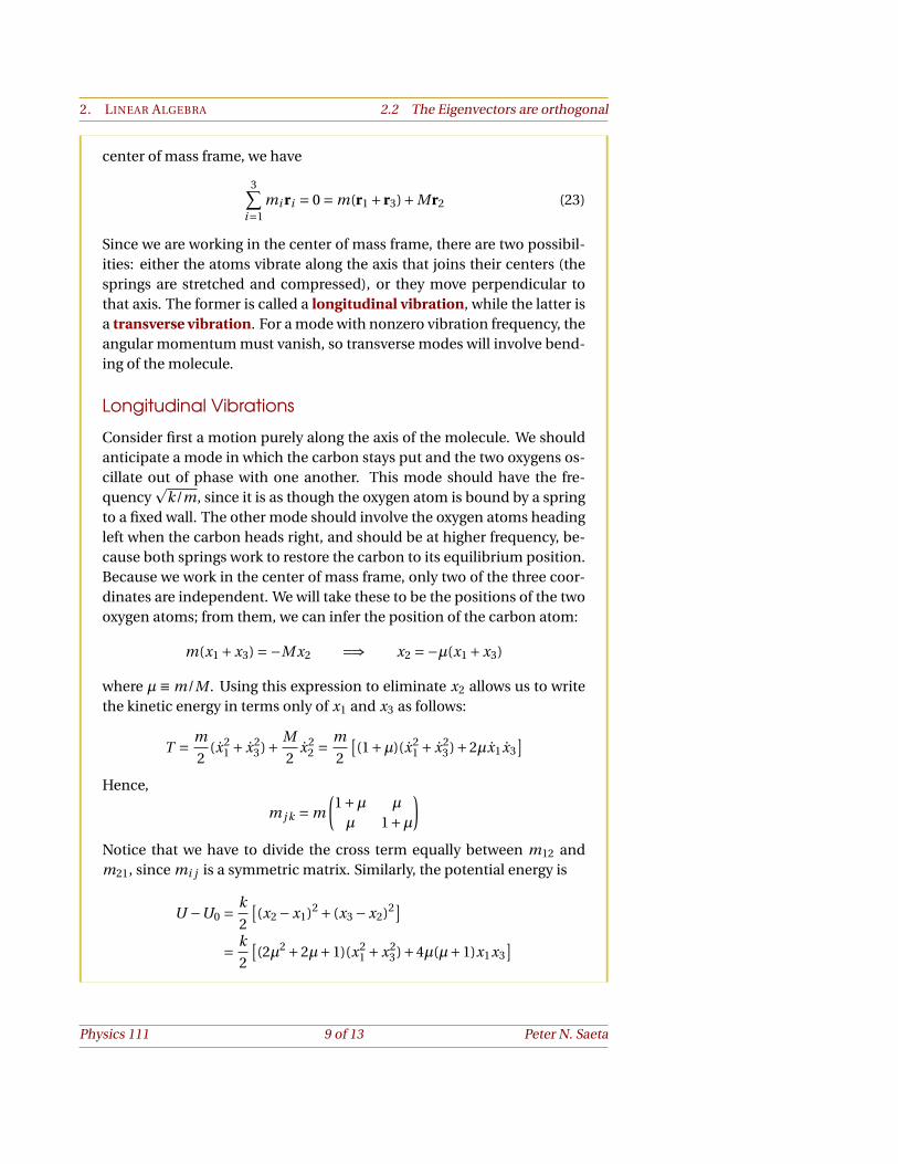
center of mass frame, we have

3∑i=1

mi ri = 0 = m(r1 + r3)+Mr2 (23)

Since we are working in the center of mass frame, there are two possibil-ities: either the atoms vibrate along the axis that joins their centers (thesprings are stretched and compressed), or they move perpendicular tothat axis. The former is called a longitudinal vibration, while the latter isa transverse vibration. For a mode with nonzero vibration frequency, theangular momentum must vanish, so transverse modes will involve bend-ing of the molecule.

Longitudinal Vibrations

Consider first a motion purely along the axis of the molecule. We shouldanticipate a mode in which the carbon stays put and the two oxygens os-cillate out of phase with one another. This mode should have the fre-quency

pk/m, since it is as though the oxygen atom is bound by a spring

to a fixed wall. The other mode should involve the oxygen atoms headingleft when the carbon heads right, and should be at higher frequency, be-cause both springs work to restore the carbon to its equilibrium position.Because we work in the center of mass frame, only two of the three coor-dinates are independent. We will take these to be the positions of the twooxygen atoms; from them, we can infer the position of the carbon atom:

m(x1 +x3) =−M x2 =⇒ x2 =−µ(x1 +x3)

where µ ≡ m/M . Using this expression to eliminate x2 allows us to writethe kinetic energy in terms only of x1 and x3 as follows:

T = m

2(x2

1 + x23)+ M

2x2

2 = m

2

[(1+µ)(x2

1 + x23)+2µx1x3

]Hence,

m j k = m

(1+µ µ

µ 1+µ)

Notice that we have to divide the cross term equally between m12 andm21, since mi j is a symmetric matrix. Similarly, the potential energy is

U −U0 = k

2

[(x2 −x1)2 + (x3 −x2)2]

= k

2

[(2µ2 +2µ+1)(x2

1 +x23)+4µ(µ+1)x1x3

]



so

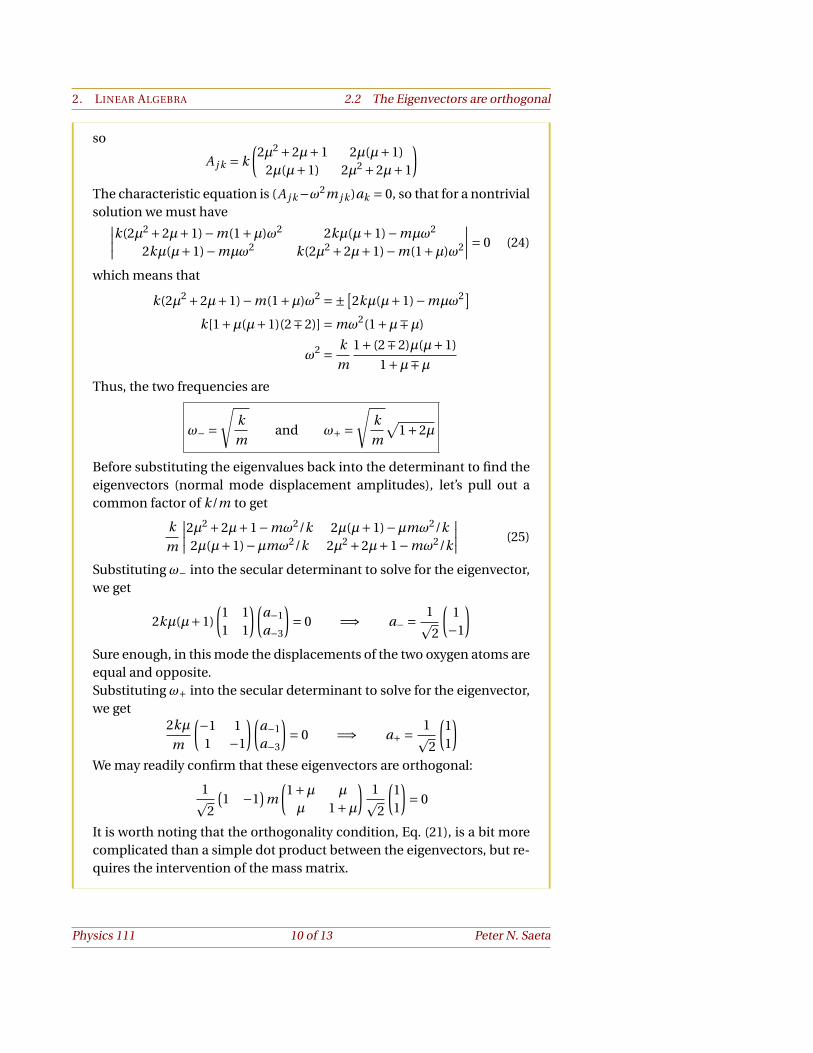
A j k = k

(2µ2 +2µ+1 2µ(µ+1)

2µ(µ+1) 2µ2 +2µ+1

)The characteristic equation is (A j k−ω2m j k )ak = 0, so that for a nontrivialsolution we must have∣∣∣∣k(2µ2 +2µ+1)−m(1+µ)ω2 2kµ(µ+1)−mµω2

2kµ(µ+1)−mµω2 k(2µ2 +2µ+1)−m(1+µ)ω2

∣∣∣∣= 0 (24)

which means that

k(2µ2 +2µ+1)−m(1+µ)ω2 =±[2kµ(µ+1)−mµω2]

k[1+µ(µ+1)(2∓2)] = mω2(1+µ∓µ)

ω2 = k

m

1+ (2∓2)µ(µ+1)

1+µ∓µThus, the two frequencies are

ω− =√

k

mand ω+ =

√k

m

√1+2µ

Before substituting the eigenvalues back into the determinant to find theeigenvectors (normal mode displacement amplitudes), let’s pull out acommon factor of k/m to get

k

m

∣∣∣∣2µ2 +2µ+1−mω2/k 2µ(µ+1)−µmω2/k2µ(µ+1)−µmω2/k 2µ2 +2µ+1−mω2/k

∣∣∣∣ (25)

Substituting ω− into the secular determinant to solve for the eigenvector,we get

2kµ(µ+1)

(1 11 1

)(a−1

a−3

)= 0 =⇒ a− = 1p

2

(1−1

)Sure enough, in this mode the displacements of the two oxygen atoms areequal and opposite.Substituting ω+ into the secular determinant to solve for the eigenvector,we get

2kµ

m

(−1 11 −1

)(a−1

a−3

)= 0 =⇒ a+ = 1p

2

(11

)We may readily confirm that these eigenvectors are orthogonal:

1p2

(1 −1

)m

(1+µ µ

µ 1+µ)

1p2

(11

)= 0

It is worth noting that the orthogonality condition, Eq. (21), is a bit morecomplicated than a simple dot product between the eigenvectors, but re-quires the intervention of the mass matrix.



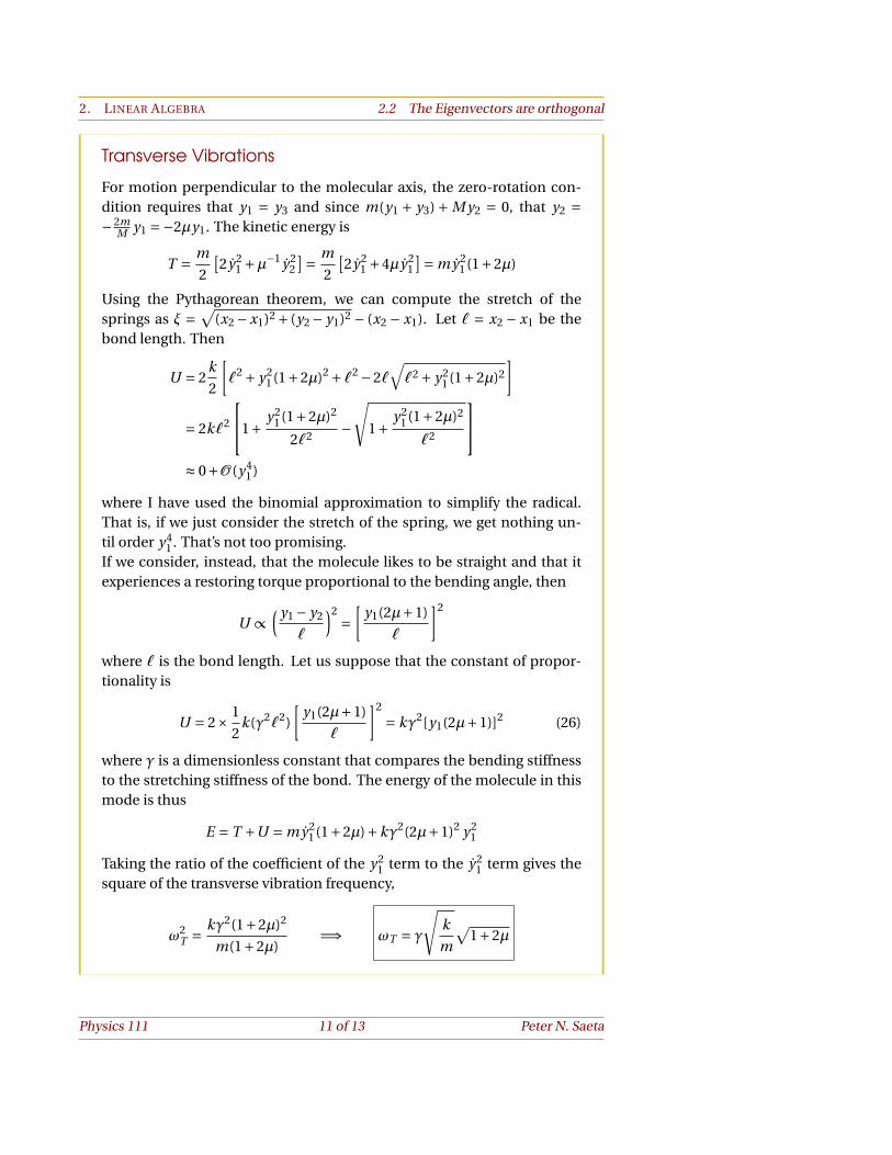
Transverse Vibrations

For motion perpendicular to the molecular axis, the zero-rotation con-dition requires that y1 = y3 and since m(y1 + y3) + M y2 = 0, that y2 =−2m

M y1 =−2µy1. The kinetic energy is

T = m

2

[2y2

1 +µ−1 y22

]= m

2

[2y2

1 +4µy21

]= my21(1+2µ)

Using the Pythagorean theorem, we can compute the stretch of thesprings as ξ =

√(x2 −x1)2 + (y2 − y1)2 − (x2 − x1). Let ` = x2 − x1 be the

bond length. Then

U = 2k

2

[`2 + y2

1(1+2µ)2 +`2 −2`√`2 + y2

1(1+2µ)2

]

= 2k`2

1+ y21(1+2µ)2

2`2 −√

1+ y21(1+2µ)2

`2

≈ 0+O (y4

1)

where I have used the binomial approximation to simplify the radical.That is, if we just consider the stretch of the spring, we get nothing un-til order y4

1 . That’s not too promising.If we consider, instead, that the molecule likes to be straight and that itexperiences a restoring torque proportional to the bending angle, then

U ∝( y1 − y2

`

)2=

[y1(2µ+1)

`

]2

where ` is the bond length. Let us suppose that the constant of propor-tionality is

U = 2× 1

2k(γ2`2)

[y1(2µ+1)

`

]2

= kγ2[y1(2µ+1)]2 (26)

where γ is a dimensionless constant that compares the bending stiffnessto the stretching stiffness of the bond. The energy of the molecule in thismode is thus

E = T +U = my21(1+2µ)+kγ2(2µ+1)2 y2

1

Taking the ratio of the coefficient of the y21 term to the y2

1 term gives thesquare of the transverse vibration frequency,

ω2T = kγ2(1+2µ)2

m(1+2µ)=⇒ ωT = γ

√k

m

√1+2µ



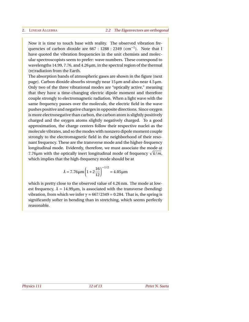
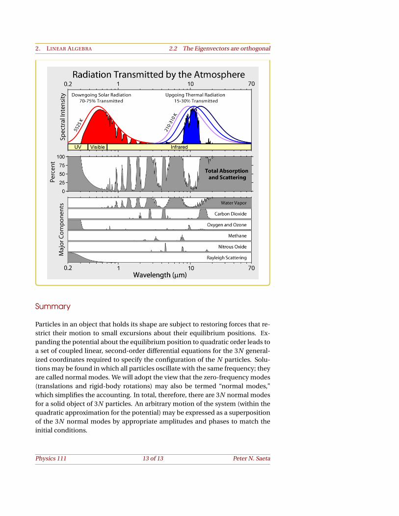
Now it is time to touch base with reality. The observed vibration fre-quencies of carbon dioxide are 667 : 1288 : 2349 (cm−1). Note that Ihave quoted the vibration frequencies in the unit chemists and molec-ular spectroscopists seem to prefer: wave numbers. These correspond towavelengths 14.99, 7.76, and 4.26µm, in the spectral region of the thermal(re)radiation from the Earth.The absorption bands of atmospheric gases are shown in the figure (nextpage). Carbon dioxide absorbs strongly near 15µm and also near 4.5µm.Only two of the three vibrational modes are “optically active,” meaningthat they have a time-changing electric dipole moment and thereforecouple strongly to electromagnetic radiation. When a light wave with thesame frequency passes over the molecule, the electric field in the wavepushes positive and negative charges in opposite directions. Since oxygenis more electronegative than carbon, the carbon atom is slightly positivelycharged and the oxygen atoms slightly negatively charged. To a goodapproximation, the charge centers follow their respective nuclei as themolecule vibrates, and so the modes with nonzero dipole moment couplestrongly to the electromagnetic field in the neighborhood of their reso-nant frequency. These are the transverse mode and the higher-frequencylongitudinal mode. Evidently, therefore, we must associate the mode at7.76µm with the optically inert longitudinal mode of frequency

pk/m,

which implies that the high-frequency mode should be at

λ= 7.76µm

(1+2

16

12

)−1/2

= 4.05µm

which is pretty close to the observed value of 4.26 nm. The mode at low-est frequency, λ = 14.99µm, is associated with the transverse (bending)vibration, from which we infer γ≈ 667/2349 = 0.284. That is, the spring issignificantly softer in bending than in stretching, which seems perfectlyreasonable.



Summary

Particles in an object that holds its shape are subject to restoring forces that re-strict their motion to small excursions about their equilibrium positions. Ex-panding the potential about the equilibrium position to quadratic order leads toa set of coupled linear, second-order differential equations for the 3N general-ized coordinates required to specify the configuration of the N particles. Solu-tions may be found in which all particles oscillate with the same frequency; theyare called normal modes. We will adopt the view that the zero-frequency modes(translations and rigid-body rotations) may also be termed “normal modes,”which simplifies the accounting. In total, therefore, there are 3N normal modesfor a solid object of 3N particles. An arbitrary motion of the system (within thequadratic approximation for the potential) may be expressed as a superpositionof the 3N normal modes by appropriate amplitudes and phases to match theinitial conditions.


Coupled Oscillators - Harvey Mudd...

Documents

Transcript of Coupled Oscillators - Harvey Mudd...