1 Elements of Markov Chain Structure and Convergence

1.1 Definition

• Random quantities x in a p−dimensional state space χ are generated sequentially according to aconditional or transition distribution P (x|x′), sometimes referred to as a transition kernel (and withseveral notations), that is defined for all x, x′ ∈ χ. The sequence of quantities x(1), x(2), . . . , x(t), . . . ,is generated from some initial value x(0) via

x(t) ∼ P (x|x(t−1)) with x(t) ⊥⊥ x(t−k)|x(t−1), (k > 1). (1)

The sequence {x(t)} is a first-order Markov process, or Markov chain, on the state space χ.

• Work in terms of density functions: whether the state space is discrete, continuous or mixed (as isoften the case in statistical modelling applications), use p(x|x′) to denote the density of P (x|x′),assuming the p.d.f. to be well-defined and unique. Then the Markov process is generated from theinitial value x(0) by convolutional sampling, i.e., sequencing through the conditionals

x(t) ∼ p(x|x(t−1))

for all t > 0.

• In this set-up, the Markov process is homogenous: for all t, transitions from x(t−1) to x(t) are governedby the same conditional distribution P (·|·). More general, non-homogenous Markov processes arealso of interest, and quite frequently used in statistical work too: that is, processes defined by transitiondensities pt(x|x′) at step t. Restrict attention here, however, to homogenous processes as much of theuse of simulation methodology in MCMC applications involves homogenous processes.

1.2 Transitions and Ergodocity

Markov processes define sequences of conditional distributions for k−step ahead transitions via convolu-tions. In the homogenous Markov chain, we have transition densities simply induced by the specified 1−steptransition density. Define the k−step transition p.d.f. pk(x|x′), for each k ≥ 1, as the conditional density ofthe state x = x(t+k) given the state x′ = x(t) for any time t. Then pk(·|·) is just the k−fold convolution ofthe transition p.d.f. p(·|·). In detail,

• p1(x(t+1)|x(t)) ≡ p(x(t+1)|x(t));• p2(x(t+2)|x(t)) =

∫p(x(t+2)|x(t+1))p(x(t+1)|x(t))dx(t+1);

• p3(x(t+3)|x(t)) =∫

p(x(t+3)|x(t+2))p2(x(t+2)|x(t))dx(t+2),

and so on with, in general,

• pk(x(t+k)|x(t)) =∫

p(x(t+k)|x(t+k−1))pk−1(x(t+k−1)|x(t))dx(t+k−1).

These densities describe the probability structure governing the evolution of the process through time stepsas a function of the core 1−step transitions. Notice that the process will be free to “wander” anywherein the state space - with positive density on any values x(t+k) ∈ χ based on any starting value x(t) - ifthe k−step density function pk(x|x′) is positive for all x, x′ ∈ χ and all k. This will be ensured, as asufficient condition and a key example, when p(x|x′) > 0 for all x, x′ ∈ χ, for example. Processes with thisproperty are generally well-behaved in the sense of defining stationary processes, under additional (weak)assumptions. This positivity condition p(x|x′) > 0 for any x, x′ ∈ χ is often true in statistical applicationsand in using MCMC methods, and will be assumed for much of our discussion.

1

The Markov process is irreducible if, starting at any initial state x′, the process can reach any other statex ∈ χ. Irreducibility is formally defined in terms of the k−step transition probabilities on subsets of χ : forany two subsets A ⊆ χ and A′ ⊆ χ, the chain is irreducible if the probability of reaching any state x ∈ Astarting from any state x′ ∈ A′ is positive under the k−step transition distribution for some finite k. Looselyspeaking, starting at any state we have positive probability of reaching any other state in a finite number ofsteps.

The process is aperiodic if – for any sets A ⊆ χ – it can move to x ∈ A in one step when starting atsome point x′ ∈ A. This is clearly also implied if p(x|x′) > 0 for all x, x′, so chains with this positivityproperty are irreducible and aperiodic.

The practical relevance of irreducibility and aperiodicity is that chains with these properties are con-vergent: in this context with p(x|x′) > 0 everywhere, we have an irreducible, aperiodic Markov processotherwise referred to as an ergodic process. Ergodic Markov processes are the main class of stationary,convergent processes of interest in MCMC. An ergodic Markov process is convergent in that the x valuesthey generate ultimately represent draws from a stationary marginal distribution. i.e., the Markov chainconverges to a stationary distribution.1

1.3 Stationary Distributions and Convergence

The Markov process has a stationary or invariant distribution Π(x), with density π(x), if

π(x) =∫

p(x|x′)π(x′)dx′.

More formally in terms of distribution functions, P (x) =∫

P (x|x′)dΠ(x′).In statistical applications of MCMC, we generally design Markov chain generating processes with a

specific stationary distribution in mind from the context of the statistical model - in a Bayesian posterioranalysis, the stationary distribution will be a target posterior distribution of interest. Note the implicationthat, if the “current state” x′ of the chain is known to be distributed according to π(x′), then the transition tothe next state maintains that marginal distribution, in that x is also distributed according to π(x). The jointdensity is p(x|x′)π(x′).

Note also that, by repeat application of the above defining identity,

π(x) =∫

pk(x|x′)π(x′)dx′

for all k ≥ 0. This is, starting with a draw from the stationary distribution will maintain the process “in” thestationary distribution forever.

If we know that the process is ergodic then π(x) is the unique stationary distribution. In such processes:

• pk(x|x′)→ π(x) as k →∞ from any initial value x′, so that the process converges in the sense that,looking ahead from any initial state x′, the probability distribution on future states x looks more andmore like the stationary distribution π(x) as k increases. The initial value is eventually “forgotten”,and samples x(k) from such a chain will eventually resemble draws (though dependent draws) fromπ(x) : x(k) ∼ π(x) as k →∞.

1In more general Markov chain theory, there are chains whose transition distributions do not satisfy the (strong but oftensatisfied) positivity condition p(x|x′) > 0 for all x, x′ ∈ χ. For some such chains the irreducibility condition needs strengtheningto positive recurrence to ensure convergence. Positive recurrence means that, if we could run the chain starting from a state x′ ∈ A,then it would return to points A infinitely often – i.e., A would “recur” – with a finite expected number of steps for recurrence forany set of points A ∈ χ. Irreducibility and positive recurrence are equivalent in our assumed context of p(x|x′) > 0 everywhere;in other contexts where the positivity condition on p(x|x′) is not satisfied, a chain may be irreducible but not necessarily positiverecurrent, and ergodicity (hence convergence) generally requires positive recurrence.

2

• We say that the Markov process or chain converges to π(x).• Ergodic averages of process values also converge (almost surely) to their limiting expectations under

π(x), i.e., for functions h(x) that are integrable with respect to π(x),

m−1m∑

t=1

h(x(t))→∫

h(x)π(x)dx

almost surely as m → ∞. This justifies the use of samples from a long Markov chain simulation asbuilding blocks for histograms and sample estimates of features of the stationary distribution. Chainsthat are initialized at values not drawn from the stationary distribution will often be “run” for an initialperiod of time until, assumedly, convergence, and sampled values, their averages and so forth thencomputed after discarding the initial “burn-in” series.

• If x(0) ∼ π(·) then, for all t > 0, x(t) ∼ π(·); if the chain starts (or, at any time point, is restarted)with a draw from the stationary distribution, then it is already “converged” and all subsequent statescome from π(x) too.

1.4 Intuition concerning convergence

Though formal proofs are well beyond our scope here, some intuitive understanding of convergence isworth exploring. The key to the intuition is that, whatever the distributions of values of x(k) generated froma Markov process, as k increases the distributions of the values and hence the ultimate “sample paths” losethe memory and effect of the initial value. That is, pk(x|x′) depends less and less on the (arbitrary) startingvalue x′ as k increases.

Consider a chain starting at an initial point x′. Then k steps in, pk(x|x′) − π(x) will (informally) besmall for all x if the chain is converging to π(x). We can write this difference as

pk(x|x′)− π(x) =∫

pk(x|x′)π(y)dy −∫

pk(x|y)π(y)dy.

where for the first term we have done nothing, and for the second we have used the identity π(x) =∫pk(x|y)π(y)dy for all k ≥ 0. Hence

pk(x|x′)− π(x) =∫{pk(x|x′)− pk(x|y)}π(y)dy.

Intuitively, as the Markov chain loses its memory the terms in brackets in the integrand will lose theirdependence on, respectively, x′ and y in the conditioning; then {pk(x|x′)− pk(x|y)} will approach zero forall values of x and the integral will approach zero implying that pk(x|x′) ≈ π(x) as required.

Formal proofs operate on differences between the probability distributions rather than densities, ofcourse. Look at any set A ⊆ χ and integrate over x ∈ A to get (with a slight abuse of notation)

P k(A|x′)−Π(A) =∫{P k(A|x′)− P k(A|y)}π(y)dy

where P k(A|x′) is the probability in A under pk(·|x′) and Π(A) that under π(·). Then, in terms of the totalvariation distance measure

‖ P k(·|x′)−Π(·) ‖= supA⊆χ|P k(A|x′)−Π(A)|,

and using the triangle inequality, we have

‖ P k(·|x′)−Π(·) ‖≤∫‖ P k(·|x′)− P k(·|y) ‖ π(y)dy.

3

The loss of dependence on the starting value x′ or any other value y ∈ χ means that the difference ofprobabilities in the integrand becomes small as k →∞, resulting in

limk→∞

‖ P k(·|x′)−Π(·) ‖= 0,

i.e., convergence of the distributions generating the values of the Markov process to the stationary distribu-tion in the sense of total variation distance.

Often the chain is geometrically ergodic, which means that

‖ P k(·|x′)−Π(·) ‖≤ cλk

for some constants c > 0 and 0 < λ < 1. Then λ represents the rate of convergence.

1.5 Reversibility and Detailed Balance

Some Markov processes are reversible, in that the transitions “backwards” in time are governed by thesame distribution p(x|x′) as the “forward” transitions. This is true of many practicable MCMC methods instatistical analysis. Clearly the chain is Markov in reverse time. In an ergodic chain with stationary densityπ(x), the “backward transition” density from a current state x(t) is available directly from Bayes’ theorem;denoting the density at time t by pr(x′|x), (r stands for reversed) we have

pr(x(t−1)|x(t)) = p(x(t−1))p(x(t)|x(t−1))/p(x(t))

where p(x(s)) denotes the density of the state at time s. In general this backward transition depends on t andso the backward chain is non-homogenous. However, if the forward chain is assumed to have convergedto its stationary distribution, or has been initialized to ensure that, then p(x(s)) = π(x(s)) and the 1-stepbackward transition p.d.f. is

pr(x(t−1)|x(t)) = π(x(t−1))p(x(t)|x(t−1))/π(x(t)).

The “backwards” process is then also homogenous, i.e., is given for all t by the transition p.d.f.

pr(x′|x) = π(x′)p(x|x′)/π(x).

Sometimes we have pr(x′|x) ≡ p(x′|x), and the Markov process is said to be reversible. In such cases,we see that

p(x′|x)π(x) = p(x|x′)π(x′),

an equation referred to historically as detailed balance. In this case, the above identity defines the symmetricjoint density of two consecutive states x, x′, in either forward or reverse directions, in the stationary process.

Some useful MCMC processes are not reversible (such as most Gibbs samplers), though some of thefocus in development of MCMC methods is to define rapidly convergent, reversible processes with specified“target” stationary distributions. One interest in reversible processes is that reversibility generally implies aunique stationary distribution (see exercises) so that convergence is often trivially assured.

1.6 Revisiting Examples

• The simple AR(1) process xt ← AR(1|θ) is an example of an ergodic, reversible Markov processwith state space the real line, when |φ| < 1. Transitions are governed by (x|x′) ∼ N(φx′, v) and thestationary distribution is x ∼ N(0, s) with s = v/(1 − φ2). The convergence rate is geometric: like|φk| as k →∞.

4

• Consider the simple Cauchy AR(1) process defined by xt = φxt−1 + εt where εt ∼ C(0, v) with|φ| < 1 and v > 0. Transitions are defined by p(x|x′) ∝ {1 + (x − x′)2/v}−1 and the process isergodic with some stationary density π(x) satisfying

π(x) ∝∫ ∞

−∞π(x′){1 + (x− x′)2/v}−1dx′.

This is not an easy equation to solve for π(x). However, the model is trivially amenable to solutionusing characteristic functions (Fourier transforms), as follows.

The characteristic function (c.f.) of any random variable z is f(s) = E(exp(isz)) and is unique. Weknow, for example, that the c.f. of C(0, v) is the function exp(−

√v|s|). Now, from xt = φxt−1 + εt

and the independence of xt−1 and εt we have

E(exp(isxt)) = E(exp(isφxt−1))E(exp(isεt)),

orfπ(s) = fπ(φs) exp(−

√v|s|),

where fπ(s) is the characteristic function of the stationary distribution. We can now simply observethat, the choice fπ(s) = exp(−

√r|s|) is a solution if, and only if,

√r =√

v/(1− |φ|). Since the c.f.of a distribution is unique, this must be the only solution, and note that it corresponds to the C(0, r)distribution; that is, we have shown that

π(x) ∝ {1 + x2/r}−1

where r = v/(1− |φ|)2.The comparison with the normal model is of interest, and we note that there are generalizations inwhich εt follows a stable distribution - distributions whose tailweights span the range between thenormal (light) and Cauchy (very heavy). These are distributions in which the c.f. is exp(−

√v|s|α)

for some index 1 ≤ α ≤ 2.

We have a suspicion - from empirical exploration of sample paths generated from such models - thatthe process is not reversible, and it is now demonstrably true: pr(x′|x) = π(x′)p(x|x′)/π(x) doesnot reduce to the forward transition p.d.f. p(x′|x). In fact, among all linear processes, of which theAR(1) is the simplest case, only normal innovations lead to reversibility. On the other hand, manyreversible non-linear processes arise routinely in MCMC (though many MCMC-derived processes arenot reversible).

2 Introduction to MCMC via Gibbs Sampling

Markov chain Monte Carlo (MCMC) methods simulate dependent sequences of random variables with thegoal of generating samples from a stationary Markov process, so that - ultimately - such values representdraws from the stationary distribution of the Markov process. MCMC algorithms are therefore created witha specific, target stationary distribution in mind, and the methodology focuses on how to develop specificMarkov chains with that stationary distribution. Explicitly, such analysis generate dependent samples, notindependent draws, and some attention there rests on the theory and methods of stationary processes andtime series analysis to investigate such methods.

5

2.1 A Simple Example

Suppose (x, y) has a bivariate normal distribution, with x ∼ N(0, 1), y ∼ N(0, 1) and C(x, y) = ρ.The following algorithm generates a sequence of values of x, namely x(1), x(2), . . . , x(t), . . . : Write r =1 − ρ2 for the conditional variance of each of the conditional distributions, (x|y) ∼ N(ρy, r) and (y|x) ∼N(ρx, r).

• Choose any value x = x(0).

• For t = 1, 2, . . . , repeat:

– Sample a value y = y(t) from the conditional distribution (y|x) at the “current” value of x =x(t−1); that is, generate a draw y(t)|x(t−1) ∼ N(ρx(t−1), r).

– Sample x = x(t) from the univariate conditional p(x|y) at the “current” value of y = y(t); thatis, draw x(t)|y(t) ∼ N(ρy(t), r).

– Save the value of x(t) and continue.

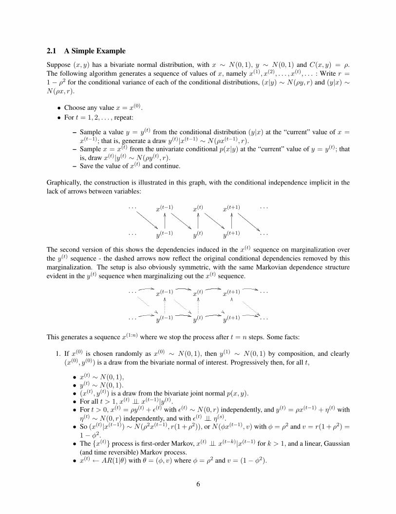
Graphically, the construction is illustrated in this graph, with the conditional independence implicit in thelack of arrows between variables:

· · ·

""EEEE

EEEE

E x(t−1)

""FFFFFFFF x(t)

""FFFFFFFF x(t+1)

""EEEE

EEEE

E· · ·

· · · y(t−1)

OO

y(t)

OO

y(t+1)

OO

· · ·

The second version of this shows the dependencies induced in the x(t) sequence on marginalization overthe y(t) sequence - the dashed arrows now reflect the original conditional dependencies removed by thismarginalization. The setup is also obviously symmetric, with the same Markovian dependence structureevident in the y(t) sequence when marginalizing out the x(t) sequence.

· · ·

""

,,x(t−1)

""

++x(t)

""

,,x(t+1)

""

** · · ·

· · ·,,y(t−1)

OO

++y(t)

OO

,,y(t+1)

OO

** · · ·

This generates a sequence x(1:n) where we stop the process after t = n steps. Some facts:

1. If x(0) is chosen randomly as x(0) ∼ N(0, 1), then y(1) ∼ N(0, 1) by composition, and clearly(x(0), y(0)) is a draw from the bivariate normal of interest. Progressively then, for all t,

• x(t) ∼ N(0, 1),• y(t) ∼ N(0, 1).• (x(t), y(t)) is a draw from the bivariate joint normal p(x, y).• For all t > 1, x(t) ⊥⊥ x(t−1)|y(t).• For t > 0, x(t) = ρy(t) + ε(t) with ε(t) ∼ N(0, r) independently, and y(t) = ρx(t−1) + η(t) with

η(t) ∼ N(0, r) independently, and with ε(t) ⊥⊥ η(s).• So (x(t)|x(t−1)) ∼ N(ρ2x(t−1), r(1 + ρ2)), or N(φx(t−1), v) with φ = ρ2 and v = r(1 + ρ2) =

1− φ2.• The {x(t)} process is first-order Markov, x(t) ⊥⊥ x(t−k)|x(t−1) for k > 1, and a linear, Gaussian

(and time reversible) Markov process.• x(t) ← AR(1|θ) with θ = (φ, v) where φ = ρ2 and v = (1− φ2).

6

• The stationary distribution of the Markov chain is the margin x(t) ∼ N(0, 1), and the sequenceof values x(1:n) generated is such that each x(t) comes from this stationary distribution, but theyare not independent: C(x(t), x(t−k)) = φk = ρ2k.• Unless φ is very close to φ = 1, these correlations decay fast with k, so that samples some

time units apart will have weaker and weaker correlations. In a long sequence, selecting out asubsequence at a given spacing of some k units, e.g., {x(0), x(k), x(2k), . . . , x(mk)} will generatea set of m draws that represent an approximately independent N(0, 1) sample if k is large enoughso that ρ2k is “negligible”.

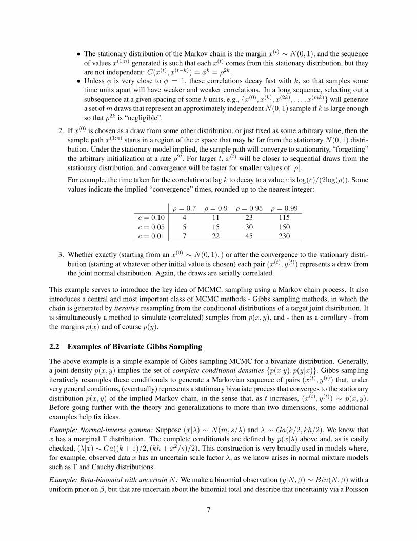
2. If x(0) is chosen as a draw from some other distribution, or just fixed as some arbitrary value, then thesample path x(1:n) starts in a region of the x space that may be far from the stationary N(0, 1) distri-bution. Under the stationary model implied, the sample path will converge to stationarity, “forgetting”the arbitrary initialization at a rate ρ2t. For larger t, x(t) will be closer to sequential draws from thestationary distribution, and convergence will be faster for smaller values of |ρ|.For example, the time taken for the correlation at lag k to decay to a value c is log(c)/(2log(ρ)). Somevalues indicate the implied “convergence” times, rounded up to the nearest integer:

ρ = 0.7 ρ = 0.9 ρ = 0.95 ρ = 0.99c = 0.10 4 11 23 115c = 0.05 5 15 30 150c = 0.01 7 22 45 230

3. Whether exactly (starting from an x(0) ∼ N(0, 1), ) or after the convergence to the stationary distri-bution (starting at whatever other initial value is chosen) each pair (x(t), y(t)) represents a draw fromthe joint normal distribution. Again, the draws are serially correlated.

This example serves to introduce the key idea of MCMC: sampling using a Markov chain process. It alsointroduces a central and most important class of MCMC methods - Gibbs sampling methods, in which thechain is generated by iterative resampling from the conditional distributions of a target joint distribution. Itis simultaneously a method to simulate (correlated) samples from p(x, y), and - then as a corollary - fromthe margins p(x) and of course p(y).

2.2 Examples of Bivariate Gibbs Sampling

The above example is a simple example of Gibbs sampling MCMC for a bivariate distribution. Generally,a joint density p(x, y) implies the set of complete conditional densities {p(x|y), p(y|x)}. Gibbs samplingiteratively resamples these conditionals to generate a Markovian sequence of pairs (x(t), y(t)) that, undervery general conditions, (eventually) represents a stationary bivariate process that converges to the stationarydistribution p(x, y) of the implied Markov chain, in the sense that, as t increases, (x(t), y(t)) ∼ p(x, y).Before going further with the theory and generalizations to more than two dimensions, some additionalexamples help fix ideas.

Example; Normal-inverse gamma: Suppose (x|λ) ∼ N(m, s/λ) and λ ∼ Ga(k/2, kh/2). We know thatx has a marginal T distribution. The complete conditionals are defined by p(x|λ) above and, as is easilychecked, (λ|x) ∼ Ga((k + 1)/2, (kh + x2/s)/2). This construction is very broadly used in models where,for example, observed data x has an uncertain scale factor λ, as we know arises in normal mixture modelssuch as T and Cauchy distributions.

Example: Beta-binomial with uncertain N : We make a binomial observation (y|N, β) ∼ Bin(N, β) with auniform prior on β, but that are uncertain about the binomial total and describe that uncertainty via a Poisson

7

distribution, N ∼ Po(m), with N ⊥⊥ β. We have the joint posterior p(β, N |y) under which the completeconditionals are

• the standard beta posterior (β|N, y) ∼ Be(1 + y, 1 + N − y), and• p(N |β, y) ∝ p(N)p(y|n, β) = constant{m(1 − β)}N−y/(N − y)!, for N ≥ y. This implies that

N = y + n where n ∼ Po(m(1− β)), with full conditional density

p(N |β, y) = {m(1− β)}N−y exp(−m(1− β))/(N − y)!, (N ≥ y).

This is an example of a bivariate posterior density in a Bayesian analysis, and one in which Gibbssampling applies trivially to simulate sequences (β(t), N (t)) that will converge to samples from thejoint posterior p(β, N |y). It is also an example where the state space of the implied Markov chain isboth discrete (N) and continuous (β), whereas all examples so far have been continuous.

2.3 Bivariate Gibbs Sampling in General

In the general bivariate case, Gibbs sampling sequences through the simulations as detailed in the normalexample above: for t = 1, 2, . . . , a draw from the (y|x) conditional simulates (y(t)|x(t−1)), then a drawfrom the (x|y) conditional simulates a new value of (x(t)|y(t)), and the process continues. We need aslightly modified notation for clarity in the theoretical development. Write the complete conditionals nowas

{px|y(·|·), py|x(·|·)}.Then Gibbs sampling generates, for all t ≥ 1, from

• y(t) ∼ py|x(·|x(t−1)), then• x(t) ∼ px|y(·|y(t)), and so on.

This defines a first-order Markov process on the (x, y) space jointly, but also univariate Markov processeson x and y individually. Consider the simulated x process x(1:n) = {x(1), . . . , x(n)} arising. We can seethat the one-step transition p.d.f. is just

p(x(t)|x(t−1)) =∫

px|y(x(t)|u)py|x(u|x(t−1))du.

Under very weak conditions, which are basically ensured in cases when the complete conditionals are com-patible with a joint and the transition p.d.f. above is positive for all x(t−1), x(t), the resulting chain willrepresent a stationary process with limiting stationary distribution given by p(x) =

∫p(x, y)dy. Conver-

gence to stationarity from an arbitrary initial value x(0) will generally be hastened if the initial value canbe chosen or simulated from a distribution close to the marginal p(x), of course, as in the bivariate normalexample.

Evidently transitions in the joint space are governed by the bivariate transition p.d.f.

p((x(t), y(t))|(x(t−1), y(t−1))) = px|y(x(t)|y(t))py|x(y(t)|x(t−1)).

2.4 Complete Conditional Specification in Bivariate Distributions

• Continue with the simple bivariate context and working in terms of density functions. Gibbs samplingin statistical analysis is commonly used to explore and simulation posterior distributions, so thatthe generic p(x, y) is then a posterior density for (x, y) from some statistical model, often definedvia Bayes’s theorem. The complete conditionals {p(x|y), p(y|x)} can then be just “read off” byinspection of p(x, y), and all is well so long as this is a proper, joint integrable density function. Notethat, as will often be the case, the joint density may be known only up to a constant of normalization.

8

• Under broadly applicable conditions, a joint density is uniquely defined by the specification of thecomplete conditionals (Theorem 7.1.19 of Robert and Casella). Given p(x|y) and p(y|x), we candeduce

p(y)∫

p(x|y)p(y|x)

dx = 1

so that p(y) is defined directly by the reciprocal of the integral of ratio of conditionals. A similar resultexists for p(x). Hence the conditionals define p(y) (and/or p(x)) and the joint density is deduced:p(x, y) = p(x|y)p(y). The requirement is simply that the integral here exists and that its reciprocaldefines a proper density function for p(y), with a parallel condition for the corresponding integraldefining p(x).• An example: take (x|y) ∼ N(ρy, (1 − ρ2)v) and (y|x) ∼ N(ρx, (1 − ρ2)w) where |ρ| < 1 and

for any variances v, w. It can be easily (if a bit tediously) verified that the integral above leads to themargin y ∼ N(0, w), the corresponding margin x ∼ N(0, v), and a bivariate normal distribution for(x, y).

• A second example: If the complete conditionals are exponential with E(x|y) = y−1 and E(y|x) =x−1, then the integral diverges, and no joint distribution exists that is compatible with these condi-tionals – they are not complete conditionals of any distribution.

3 Gibbs Sampling

3.1 General Framework

Consider a p−dimensional distribution with p.d.f. p(x). Consider any partition of x into a set of q ≤ p ele-ments x = {x1, . . . , xq} where each xi may be a vector or scalar. The implied set conditional distributionshave p.d.f.s

p(xi|x−i), where x−i = x\xi, (i = 1, . . . , q). (2)

In the extreme case in which xi is univariate, these define the set of univariate complete conditional distri-butions defined by p(x). In other cases the set of q conditionals represents conditionals implied on vectorsubsets of x based on the chosen partitioning. To be clear in notation, we now subscript the conditionals bythe index of the subvector in the argument, and as needed will explicitly denote the conditioning elements,i.e.,

pi(xi|x1, . . . , xi−1, xi+1, . . . , xq) = pi(xi|x−i) ≡ p(xi|x−i)

for each i = 1, . . . , q.The idea of Gibbs sampling is just the immediate extension from the bivariate case above. With x

partitioned in the (essentially arbitrary) order as described, proceed as follows:

1. Choose any value initial value x = x(0).

2. Successively generate values x(1), x(2), . . . , x(n), as follows. For each t = 1, 2, . . . , based on the“current” value x(t) sample a new state x(t+1) by this sequence of simulations:

• draw a new value of x1, namely

x(t+1)1 ∼ p1(x1|x(t)

−1);

• continue through new draws of

x(t+1)i ∼ pi(xi|x(t+1)

1 , . . . , x(t+1)i−1 , x

(t)i+1, . . . , x

(t)q )

from i = 2, . . . , q − 1, then

9

• complete the resampling viax(t+1)

q ∼ pq(xq|x(t+1)−q ).

This results in a complete update of x(t) to x(t+1), and then passes to the next step. Note how, at eachstep, the “most recent” sampled values of each element of x in the conditioning is used.

The term Gibbs sampling has sometimes been restricted to apply to the case of p = q when all elements xi

are univariate, and the conditional distributions pi(·|·) are the full set of p complete univariate conditionals.More generally, and far more common in practice, is the use of a partition of x into a set of componentsfor which the implied q conditionals are easily simulated. It should be intuitively evident that blockingunivariate elements together into an element xi and then sampling x

(t+1)i from the implied conditional leads

to - for that block of components of x(t+1) - a simulated value that depends less on the previous valuex(t) than it would in the pure Gibbs sampling from univariate conditionals. An extreme example is whenwe have just one element, so sample directly from p(x). Theory supports this intuition: the more we canblock elements of x together to create subvectors xi of higher dimension, the weaker will be the dependencebetween successive values x(t) and x(t+1). Hence in examples from here on, and especially practical modelexamples, the MCMC iterates between parameters and variables of varying dimension. Indeed, this is reallykey to the broad applicability and power of MCMC generally, and Gibbs sampling in particular.

In the following examples, the state space is a parameter space defined in a statistical model analysis,and Gibbs sampling is used to sample from the posterior distribution in that analysis.

3.2 An Example of Gibbs Sampling Using Completion

“Completion” refers to extending the state, or parameter space to introduce otherwise hidden or latent vari-ables that, in this context, provide access to a Gibbs sampler. The term “data augmentation” is also used,although usually the additional variables introduced are not hypothetical data at all; in some cases, they do,however, have a substantive interpretation, as in problems with truly missing or censored data.

A simple, and very useful example is linear regression modelling under a heavy-tailed error distribu-tion fixes ideas. This is a special case of linear regression with heavy-tailed errors, which underlies “robustregression” estimation - the use of an error distribution that has heavier-tails than normal can provide “pro-tection” against outlying observations (bad or corrupt measurements) that, in the normal model, can havea substantial and undesirable impact on regression parameter estimation. Much empirical experience sup-ports the view that, in many areas of science, natural and experimental processes generate variation that,while leading to (at least approximately) symmetric error distributions, is simply non-normal and usuallyheavier-tailed.

3.2.1 Reference Normal Linear Regression

Start with the usual normal linear model and its reference Bayesian analysis:

• n observations in n−vector response y, known n × k design matrix H whose columns are the nvalues of k regressors (predictor variables), and n−vector of observational errors ε with independentelements εi ∼ N(0, φ−1) of precision φ.

• Elements of y : yi = h′iβ + εi where the hi are the rows of H.

• y = Hβ + ε.

In the general notation we have a state x = (β, φ) with the corresponding p = (k + 1)−dimensional statespace. The standard reference posterior p(x|y) ≡ p(β, φ|y) is well-known:

10

• Reference prior p(β, φ) ∝ φ−1 leads to the reference posterior of a normal/inverse gamma form,namely (β|φ, y) ∼ N(b, φ−1B−1) and (φ|y) ∼ Ga((n − k)/2, q/2) where B = H ′H, b = β =B−1H ′y is the LSE, and q = e′e is the sum of squared residuals e = y −Hb.

The implied posterior T distribution for β is usually used for inference on regression effects, and this canof course be simulated if desired - most easily via the convolution implicit in the conditional normal/inversegamma posterior above. That is, the joint posterior p(β, φ|y) is directly simulated by drawing φ from itsmarginal gamma posterior and then, conditional on that φ value, drawing β from the conditional normalposterior.

3.2.2 Reference Normal Linear Regression with Known, Unequal Observational Variance Weights

Weighted linear regression (and weighted least square) has εi ∼ N(0, λ−1i φ−1) independently, allowing

differing “weights” λi to account for differing precisions in error terms. The reference analysis is triviallymodified in this case when the weights Λ = (λ1, . . . , λn)′ are specified. Now,

yi = h′iβ + εi where εi ∼ N(0, λ−1i φ−1).

The changes to the posterior are simply that, now, the regression parameter estimate b, associated precisionmatrix B and the residual sum of squares are based on the weighted design and response data, via

B = H ′ΛH, b = B−1H ′Λy and q = e′Λe.

3.2.3 Heavy-Tailed Errors in Regression

A key example is to change the normal error assumption into a T distribution, say T with ν = 5 degreesof freedom. We can imagine treating ν as an additional parameter to be estimated, but for now consider νfixed. Evidently, the joint posterior is now complicated:

p(β, φ|y) ∝ φn/2−1n∏

i=1

{1 + φ(yi − h′iβ)′(yi − h′iβ)/ν}−(ν+1)/2,

in the (k + 1)−dimensional parameter space. This is, in general, a horribly complicated (poly-T) func-tion that may be multimodal, skewed differently in different dimensions, and is very hard to explore andsummarise.

The completion, or augmentation, method that enables an almost trivial Gibbs sampler just exploits thedefinition of the T distribution as a scale mixture of normals. Recall that the T distribution for εi can bewritten as the marginal distribution from a joint in which

• εi|λi ∼ N(0, λ−1i φ−1), and

• λi ∼ Ga(ν/2, ν/2).

Write Λ = (λ1, . . . , λn)′ for the new/latent parameters induced here. Then, conditional on Λ, we have theweighted regression model. The augmentation is now clear: extend the state from (β, φ) to x = (x1, x2)with x1 = (β, φ) and x2 = Λ. The posterior of interest is now p(x1, x2|y) - if we can sample this posterior,then the simulated values lead to marginal samples for the primary parameters x1 = (β, φ), while alsoadding value in that we will generate posterior draws of the latent “weights” of observations that can beused to explore which observations have large/small weights, based on the fit to the predictors.

The two conditional posteriors of interest are defined:

11

• For x1 = (β, φ), we have the weighted regression model conditional on x2 = Λ, so we know that wesimulate directly from p(β, φ|Λ, y) via

– (φ|Λ, y) ∼ Ga((n− k)/2, q/2) and then– (β|φ,Λ, y) ∼ N(b, φ−1B−1)

where b = H ′ΛH, b = B−1H ′Λy and q = e′Λe with e = y −Hb.

• For x2 = Λ, it is trivially seen that

p(Λ|β, φ, y) =n∏

i=1

p(λi|β, φ, yi)

with independent component margins p(λi|β, φ, yi) ∝ p(λi)p(yi|β, φ, λi), so that

(λi|β, φ, yi) ∼ Ga((ν + 1)/2, (ν + φε2i )/2)

at εi = yi − h′iβ.

3.3 General Markov Chain Framework of Gibbs Sampling

Gibbs samplers define first-order Markov processes on the full p−dimensional state space. Note that thesequence of conditional simulations in §3.1 provides a complete update from the sampled vector x(t−1) tothe sampled vector x(t) by successively updating the components. That this is Markov is obvious, and itis clearly also homogenous since the conditional distributions are the same for all t. The implied transitiondistribution is easily seen to be based on these individual conditionals. For clarity in notation in this sectionwrite F (x|x′) for the transition distribution function and f(x|x′) for the corresponding p.d.f. . Then theMarkov process defined by the Gibbs sampler has transition p.d.f. governing transitions from any state x′ tonew states x, of the form:

f(x|x′) = p1(x1|x′−1){q−1∏i=2

pi(xi|x1, . . . , xi−1, x′i+1, . . . , x′q)}pq(xq|x−q).

It is relatively straightforward to show (see Robert and Casella, §7.1.3) that the joint density p(x) doesindeed provide a solution as a stationary distribution of the Markov process, i.e.,

p(x) =∫

f(x|x′)p(x′)dx′.

Further, under conditions that are every broadly applicable in statistical applications, the process convergesto this unique stationary distribution: the Markov chain defined by the Gibbs sampler is irreducible andaperiodic, so defining an ergodic process with limiting distribution p(x). Thus, MC samples generated bysuch Gibbs samplers will converge in the sense that, ultimately, x(t) ∼ p(x). This is the case in applicationswith positive conditional densities pi(xi|x−i) > 0 for all x, for example, and this really highlights therelevance and breadth of applicability in statistical modelling. There are models and examples in which thisis not the case, though even then convergent Gibbs samplers may be defined (on a case-by-case basis) oralternative methods that modify the basic Gibbs structure may apply.

In general, the Markov chains generated by Gibbs samplers are not reversible on the full state space,though the induced chains on elements of x are.

12

3.4 Some Practicalities

3.4.1 General Comments

• The key focuses in setting up and running a Gibbs sampler relate to the choice and specification ofthe conditional distributions with two considerations: ease and efficiency of the resulting simulations,and resulting dependence between successive states in the resulting Markov chain. Once a sampleris specified, the questions of monitoring it to assess convergence - to decide when to begin to savegenerated x values following an initial “burn-in” period - are raised.

• A sampler with very low dependence between successive states is generating samples that are close torandom samples, and that is the gold-standard. Highly dependent chains may be sub-sampled to savedraws some iterations apart, thus weakening the serial dependence. Setting up and running a Gibbssampler requires specification of sets of conditional distributions as in the examples, and choices aboutwhich specific distributions to use. We have already discussed the idea of blocking - using conditionaldistributions such that the subvectors xi are of maximal dimension, in an attempt to “weaken” thedependence between successively saved values.• Initialization is often challenging, and repeat Gibbs runs from different starting values are of relevance.

Repeat, differentially initialled Gibbs runs that eventually generate states in the same region suggestthat there has been convergence to that region.

• Most Gibbs samplers are non-linear, though linear autocorrelations are the simple, standard tools forexamining first-order structure. Plotting sample paths of selected subsets of x over Gibbs iterates, andplotting sample autocorrelation functions for Gibbs output series after an initial burn-in period, aretwo common exploratory methods.

3.4.2 Sample Autocorrelations

Recall the notation for dependence structure in a stationary univariate series xt. Assuming second-ordermoments exist) the autocovariance function is γ(k) = C(xt, xt±k) with marginal variance V (xt) = γ(0)for each t, and then the corresponding autocorrelation (a.c.f.) function is ρ(k) = γ(k)/γ(0). Sample auto-covariances and autocorrelations based on an observed series x1:n are just the sample analogues, namely

γ(k) = n−1n−k∑t=1

(xt − x)(xt+k − x) and ρ(k) = γ(k)/γ(0).

Simply evaluating and plotting the latter based on a (typically long, perhaps subsampled) Gibbs series givessome insights into the nature of the serial dependence. The concepts and insights into dependence overtime we have generated in studying (exhaustively) the linear AR(1) model translate into assessment of serialdependence in Gibbs samples, even though they generally represent non-linear AR processes.

nb. See course web page, under the Examples, Matlab Code and Data link, for simple Matlab functionsfor computing and plotting the a.c.f.

3.5 Gibbs Sampling in Linear Regression with Multiple Shrinkage Priors

See Supplementary Notes web page link to MW Valencia 8 tutorial slides.

3.6 Gibbs Sampling in Hierarchical Models

See Gamerman & Lopes §5.5 for some examples, and others throughout the book and in some of the refer-ences.

13

4 Gibbs Sampling in a Stochastic Volatility Model: HMMs and Mixtures

4.1 Introduction

Here is an example that both introduces very standard, core manipulation of discrete mixture distributionsand that provides a component of a nowadays standard Gibbs sampler for the non-linear stochastic volatilitymodels in financial times series. Recall the canonical SV model. We have an observed price series, suchas a stock index or exchange rate, Pt at equally spaced time points t, and model the per-period returnsrt = Pt/Pt−1 − 1 as a zero mean but time-varying volatility process

rt ∼ N(0, σ2t ),

σt = exp(µ + xt),xt ← AR(1|θ)

with θ = (φ, v). (In reality, such models are components of more useful models in which the mean ofthe returns series is non-zero and is modelled via regression on economic and financial predictors). Theparameter µ is a baseline log-volatility; the AR(1) parameter φ defines persistence in volatility, and theinnovations variance v “drives” the levels of activity in the volatility process.

Based on data r1:n, the uncertain quantities to infer are (x1:n, µ, θ) and MCMC methods will utilize agood deal of what we know about the joint normal distribution - and its various conditionals - of x0:n. Themajor complication arises due to the non-linearity inherent in the observation equation, and one approach todealing with this uses the log form earlier mentioned: transforming the data to yt = log(r2

t )/2, we have

yt = µ + xt + νt,

xt ← AR(1|θ),

where νt = log(κt)/2 and κt ∼ χ21. This is a linear AR(1) HMM but with non-normal observation errors

νt. We know that we can develop an effective Gibbs sampler for a normal AR(1) HMM, and that suggestsusing normal distributions somehow.

4.2 Normal Mixture Error Model

We know that we can approximate a defined continuous p.d.f. as accurately as desired using a discretemixture of normals. Using such a mixture for the distribution of νt provides what is nowadays a standardanalysis of the SV model, utilizing the idea of completion again - i.e., introducing additional latent variablesto provide a conditionally normal model for the νt, and then including those latent variables in the analysis.Specifically:

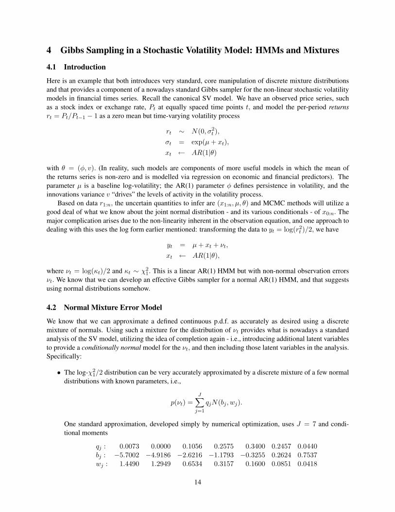
• The log-χ21/2 distribution can be very accurately approximated by a discrete mixture of a few normal

distributions with known parameters, i.e.,

p(νt) =J∑

j=1

qjN(bj , wj).

One standard approximation, developed simply by numerical optimization, uses J = 7 and condi-tional moments

qj : 0.0073 0.0000 0.1056 0.2575 0.3400 0.2457 0.0440bj : −5.7002 −4.9186 −2.6216 −1.1793 −0.3255 0.2624 0.7537wj : 1.4490 1.2949 0.6534 0.3157 0.1600 0.0851 0.0418

14

See Kim, Shephard and Chib, 1998, Review of Economic Studies for this. Mixtures with more com-ponents can refine the approximation - the Gibbs sampling setup is structurally the same, and justchanges in details.

• Introduce latent indicator variables γt ∈ {1 : J} with p(γt) = qj at γt = j independently over t andof all other random quantities. Then the mixture of normals can be constructed from the conditionals

(νt|γt = j) ∼ N(bγt , wγt) ≡ N(bj , wj), (j = 1, . . . , J).

The implied marginal distribution of νt, averaging with respect to the discrete density p(γt) is the mix-ture of normals above. This is the data augmentation, or completion, trick once again. We introducethese latent mixture component indicators to induce conditional normality of the νt.

4.3 Exploiting Conditional Normality in Normal Mixtures

Some of the key component distributions for Gibbs sampling in the normal mixture SV model are mostclearly understood by, first, pulling out of the time series context and considering just one time point - wewill drop the t suffix for clarity and for this general discussion. Conditional on (γ = j, x, µ), we havey ∼ N(µ + x + bj , wj). Imagine now that, at some point in a Gibbs sampling analysis, we are interestedin the conditional posterior for x under a normal prior and conditioning on current values of γ = j and µ.The likelihood for x in this setup is normal, so the implied conditional posterior for x is normal. Similarly,at any point in a Gibbs sampling analysis when we want to compute the conditional posterior for µ under anormal prior and conditioning on current values of γ = j and x, the likelihood for µ in this setup is normal,so the implied conditional posterior for µ is normal. Hence, we can immediately see that the imputationof the latent mixture component indicators translates the complicated model into a coupled set of normalmodels within which the theory is simple, and conditional simulations are trivial. This is the key to MCMCin this example, and many others involving mixtures.

To be explicit, if we have a prior x ∼ N(m,M) then we have the following component conditionaldistributions:

• The conditional posterior for (x|y, γ, µ) is normal with moments

– E(x|y, γ, µ) = m + A(y − µ− bγ −m) with A = M/(M + wγ) and– V (x|y, γ, µ) = wγA.

• The conditional posterior for (γ|y, x, µ) is given by the J probabilities q∗j over γ = j ∈ {1, . . . , J},via

q∗j = Pr(γ = j|y, x, µ) ∝ Pr(γ = j)p(y|γ = j, x, µ)∝ qj exp{−(y − µ− bj − x)2/(2wj)}/

√wj

for j = 1, . . . , J. Normalization over j leads to the updated probabilities q∗j .

These two, coupled conditionals are easy to simulate, and form key elements of the complete Gibbs samplerfor the normal mixture SV models.

4.4 An Initial Gibbs Sampler in the SV Model

A full Gibbs sampler can now be defined to simulate from the complete target posterior

p(x0:n, µ, φ, v|y1:n)

15

by first extending the state space to include the set of indicators γ1:n. That is, we sample various conditionalsof the full posterior

p(x0:n, γ1:n, µ, φ, v|y1:n).

One component of this will be to sample x0:n from a conditionally linear, normal AR(1) HMM, and allingredients have been covered: Question 2 of Homework #2 and Question 3 of the Midterm exam. Forthis we need to finalize the specification with the prior p(x0, µ, φ, v), and here take these quantities to beindependent with prior p(x0)p(µ)p(φ)p(v) where x0 ∼ N(0, u) for some (large?) u > 0, µ ∼ N(g,G),φ ∼ N(c, C) and v−1 ∼ Ga(a/2, av0/2).

Gibbs sampling can now be defined. One convenient initialization is to set µ = y = n−1 ∑nt=1 yt

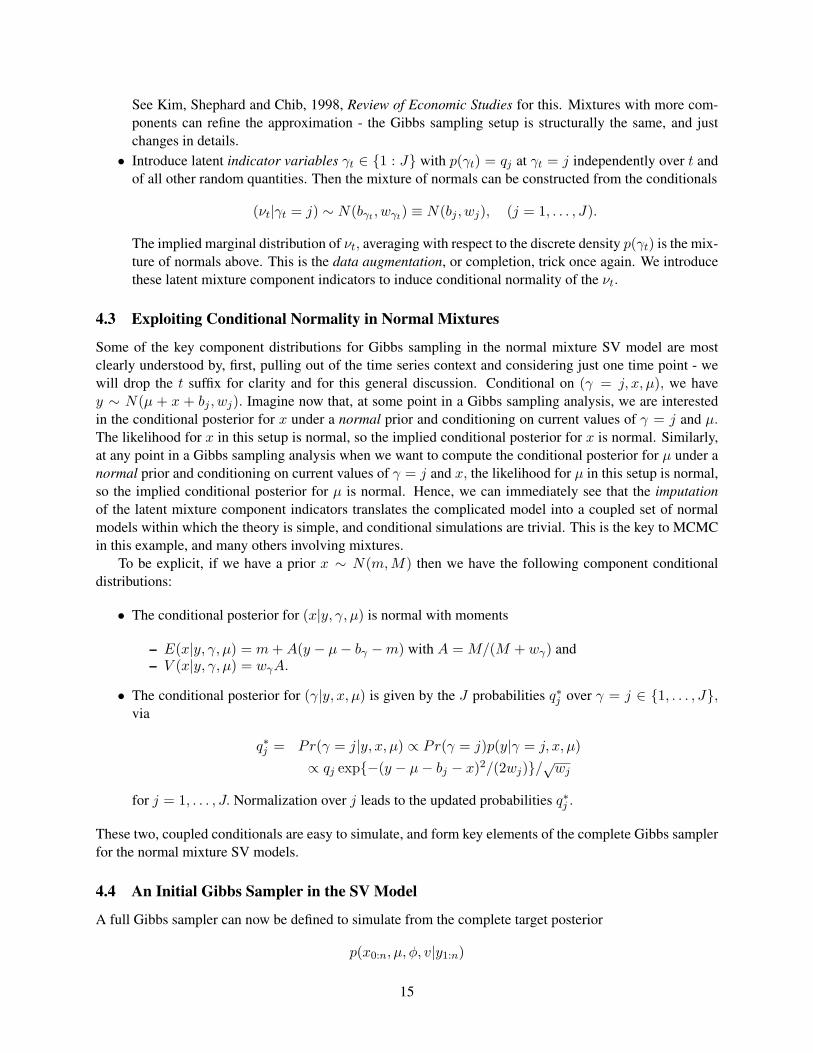
and then, for each t = 1, . . . , n, xt = yt − y and with x0 = 0. Given these initial values, the sequence ofconditionals to sample from to generate each Gibbs step is as follows. Note that each conditional distributionis, formally, explicitly conditioned on values of all other uncertain and observed quantities; however, thehighly structured model has various conditional independencies that leads to reduction and simplification ineach case. This is characteristic of Gibbs sampling in complex, hierarchical models - we massively exploitthis conditional independence structure to simplify the calculations.

The conditional independence structure is exhibited in the graphical model:

µ

������

����

����

����

�� ��666

6666

6666

6666

6

· · · γt−1

��

γt

��

γt+1

��

· · ·

· · · yt−1 yt yt+1 · · ·

· · · // xt−1

OO

// xt

OO

// xt+1

OO

// · · ·

(φ, v)

iiRRRRRRRRRRRRRRRRR

ccGGGGGGGGG

OO ;;wwwwwwwww

55lllllllllllllllll

1. p(γ1:n|y1:n, x0:n, µ, φ, v).

It is immediate that the γt are conditionally independent and the above discussion provides the condi-tional posteriors over j = 1, . . . , J. Namely,

Pr(γt = j|yt, xt, µ) = q∗t,j

whereq∗t,j ∝ qj exp{−(yt − µ− bj − xt)2/(2wj)}/

√wj

for j = 1, . . . , J, and normalization over j leads to the updated probabilities q∗t,j , for each timepoint t. This defines a discrete posterior for each γt that is trivially sampled to generate new mixturecomponent indicators.

2. p(φ|y1:n, x0:n, µ, v).

This is just the normal posterior p(φ|x0:n, v) for the AR(1) coefficient in the AR(1) model under theφ ∼ N(c, C) prior. This is trivially sampled to generate a new value of φ.

3. p(v|y1:n, x0:n, µ, φ).

This is just the posterior p(v|x0:n, φ) for the AR(1) innovation variance in the AR(1) model under theinverse gamma prior. This is trivially sampled to generate a new value of v.

16

4. p(µ|y1:n, x0:n, γ1:n, φ, v).

This is the posterior for µ under the µ ∼ N(g,G) prior and based on n conditionally normal, indepen-dent observations y∗t = yt − xt − bγt ∼ N(µ,wγt). So the posterior is, easily, normal, say N(g′, G′)where

1/G′ = 1/G + 1/W and g′ = G′(g/G + µ/W )

where

W−1 =n∑

t=1

w−1γt

and µ = Wn∑

t=1

w−1γt

y∗t .

5. p(x0:n|y1:n, γ1:n, µ, φ, v).

Under the conditioning here we have a (conditionally) linear, normal AR(1) HMM. The one extensionto the discussion of this model earlier is that, given the specific values of elements of γ1:n, the errorvariances of the normal distributions for the yt are known and different over time: the earlier constantvariance w is replaced by the conditional values wγt for each t. We can then run the forward-filtering,backward sampling (FFBS) algorithm that uses the Kalman filter-like forward analysis from t = 1up to t = n, then moves backwards in time successively simulating the states xn, xn−1, . . . , x0 togenerate a full sample x0:n.

For clarity here, temporarily drop the quantities (γ1:n, µ, φ, v) from the conditioning of distributions- they are important but, at this step, fixed at “current” values throughout.

• Forward Filtering:Refer back to Question 2 of Homework #2 for full supporting details.Beginning at t = 0 with x0 ∼ N(m0,M0) where m0 = 0,M0 = u, we have, for all t =0, 1, . . . , n, the on-line posteriors

(xt|y1:t) ∼ N(mt,Mt)

sequentially computed by the Kalman filtering update equations:

mt = at + Atet and Mt = wγtAt

where

et = yt − µ− bγt − at,

at = φmt−1,

At = ht/(ht + wγt),ht = v + φ2Mt−1.

• Backward Sampling:

– At t = n, sample from (xn|y1:n) ∼ N(mn,Mn).– Then, for each t = n− 1, n− 2, . . . , 0, sample from

p(xt|x(t+1):n, y1:n) ≡ p(xt|xt+1, y1:t)

using the just sampled value of xt+1 in the conditioning. Here (xt|xt+1, y1:t) is normal with

E(xt|xt+1, y1:t) = mt + (φMt/ht+1)(xt+1 − at+1)

andV (xt|xt+1, y1:t) = vMt/ht+1.

17

It is worth commenting on the final step and the relevance of the FFBS component. This is an exampleof a Hidden Markov Model and this specific approach is used in other such models, including HMMswith discrete state spaces. In the SV model here, an older, alternative approach to simulating the latentxt values is to use a Gibbs sampler on each of the complete conditionals p(xt|x−t, y1:n, γ1:n, µ, φ, v).This is certainly feasible and a simpler technical approach, but will tend to be much less effective inapplications, especially in cases - as in finance - where the AR dependence is high. In many suchapplications φ is close to 1, the process being highly persistent; this induces very strong correlationsbetween xt and xt−1, xt+1, for example, so that the set of complete univariate conditionals will bevery concentrated. A Gibbs sampler run on these conditionals will then move around the x componentof the state space extremely slowly, with very high dependence among successive iterations - it willconverge, but very, very slowly indeed. The FFBS approach blocks all the xt variates together and ateach Gibbs step generates a completely new sample trajectory x0:n from the relevant joint distribution,and so moves swiftly around the state space, generally rapidly converging.

4.5 Ensuring Stationarity of the SV Model

Some of the uses of the model are to simulate future volatilities: given an MC sample from the above Gibbsanalysis, it is trivial to then forward sample the xt process to generate an MC sample for, say, xn+k for anyk > 0, and hence deduce posterior samples for p(rn+k|y1:n). The spread of these distributions play intoconsiderations of just how wild future returns might be, and currently topical questions of value-at-risk infinancial management, for example.

Practical application of SV models require that we modify the set-up to ensure that the SV process isstationary. A model allowing values of |φ| > 1 will generate volatility processes that are explosive, and thatis quite unrealistic. The modification is trivial mathematically and - now that the analysis and model fittinguses Gibbs sampling - makes little difference computationally and involves only very modest changes to theabove set of conditional distributions. This is an example of how analysis using MCMC allows us to easilyovercome technical complications that would otherwise be much more challenging.

The volatility process is stationary if we restrict to |φ| < 1 and assume the stationary distribution for thepre-initial value x0. That is,

(x0|φ, v) ∼ N(0, v/(1− φ2)).

Hence, for stationarity we must replace the earlier assumption x0 ∼ N(0, u) by substituting u = v/(1−φ2).This depends on the unknown parameters (φ, v) but that simply means we need to recognize how thischanges some or all of the conditional distributions within the MCMC analysis as a result of this dependence.The impact on the set of five conditional distributions are as follows.

1. The conditional distributions for γ1:n are unchanged.2. The conditional posterior for φ is now restricted to the stationary region |φ| < 1. In volatility mod-

elling we expect high, positive values so that we may restrict further to 0 < φ < 1 if desired; we shallassume this here for the following development. Further, the posterior for φ also now has an addi-tional component contributed by the likelihood term p(x0|φ, v) that had earlier been ignored. Thusthe conditional is

p(φ|x0:n, v) ∝ p(φ)p(x1:n|x0, φ, v)p(x0|φ, v), 0 < φ < 1.

We may still use the prior p(φ) = N(c, C) but now truncated to 0 < φ < 1, so that

p(φ|x0:n, v) ∝ exp(−(φ− c′)2/(2C ′))a(φ), 0 < φ < 1,

18

where 1/C ′ = 1/C +B/v and c′ = C ′(c/C +Bb/v) with B =∑n

t=1 x2t−1 and where b is the sample

autocorrelation at lag-1, b =∑n

t=1 xtxt−1/B, as before. Also the term a(φ) is just

a(φ) ∝ p(x0|φ, v) = (1− φ2)1/2 exp(φ2x20/(2v)).

Note that this latter term introduces an additional technical complication, but is a term that apparentlycontributes little (it is “worth” one observation on the x series, compared to the other n− 1) and may,at this first step, be ignored. If we ignore a(φ), the conditional density is a truncated normal, whichwe can easily simulate. We shall see how to simply modify this using a Metropolis-Hastings MCMCcomponent later on.

3. The conditional for v is similarly modified by the addition of the pre-initial term

p(x0|φ, v) ∝ v−1/2 exp((1− φ2)x20/(2v))

now viewed as a function of v. This adds one degree-of-freedom to the conditional inverse gammaposterior, and adds the term (1 − φ2)x2

0 to the sum-of-squares; that is, under the prior v−1 ∼Ga(a/2, av0/2) based on some prior point estimate v0 and degrees-of-freedom a, we have the condi-tional posterior

(v−1|x0:n, φ) ∼ Ga((a + n + 1)/2, (av0 + q)/2)

where q = (1− φ2)x20 +

∑nt=1 ε2t with εt = xt − φxt−1 for t = 1, . . . , n.

4. The conditional distributions for µ is unchanged.5. The only change to the FFBS analysis is the initialization at x0 ∼ N(m0,M0) as described, but now

the initial moments are m0 = 0 and M0 = v/(1− φ2).

4.6 Model Re-parametrization: The Centered AR Model

The above Gibbs sampler can be usefully applied to generate exploration of the full posterior, and is provablyconvergent. However, it is an excellent example of an MCMC analysis that suffers from slow convergence insome components - specifically, the (x0:n, µ) sub-states, due to choice of parametrization. Some experiencein exploring this Gibbs sampler with either simulated or real data quickly reveal that the simulated samplepaths for µ will almost always drift far away from regions consistent with expectation under the prior and,in a financial times series analysis, with economic reality. This is coupled with corresponding drifts in thesample paths of the simulated volatility process xt itself. The problem is one of “soft” identification, and isclarified as follows. The yt data provide direct observations on the sum µ + xt. Adding any constant to µwhile subtracting that same constant from each of the xt leaves the model unchanged, so that the posteriorwill inevitably exhibit very strong negative dependence between the values of the xt process and µ. TheGibbs sampler as structured above couples sampling for µ given x0:n with sampling for x0:n given µ, andso will usually wander around generating samples such that the µ + xt are quite appropriate and consistentwith the data, but with with values of µ and xt themselves subject to quite unpredictable and commonlyvery large shifts up/down respectively. Simply applying the sampler and monitoring convergence will showclear evidence of (a) very strong negative dependence as described, and (b) high positive autocorrelationswithin the Gibbs iterates indicative of the non-stationary drifting.

This is a common problem in complex, multi-parameter models. Some examples in hierarchical modelsare discussed by Gamerman & Lopes at length (see especially §5.3.4 and §6.4.4). The practicality is one ofappropriate choice of parametrization to define the Gibbs conditional posteriors when more than one suchchoice is possible, and this example of theoretically implied dependence in the posterior - that is obviousfrom the structure of the model - is a key feature that, in other models, should suggest re-parametrization.The solution here is to focus on the centered AR(1) parametrization, as follows.

19

Write zt = µ + xt so that xt = zt − µ for each t. Then the model is recast as

yt = zt + νt,

zt = µ + φ(zt−1 − µ) + εt,

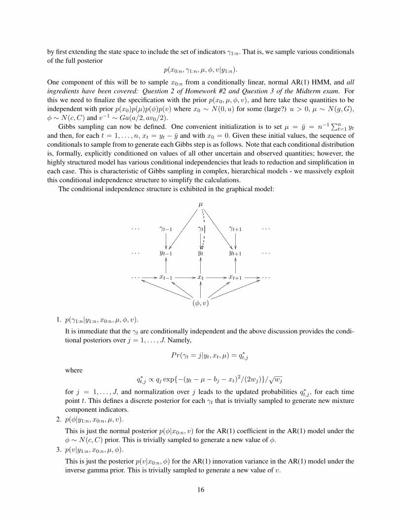
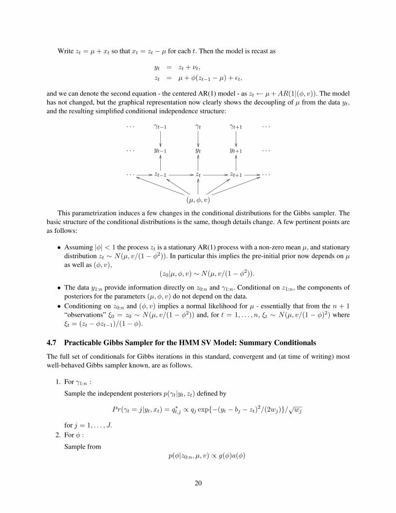
and we can denote the second equation - the centered AR(1) model - as zt ← µ + AR(1|(φ, v)). The modelhas not changed, but the graphical representation now clearly shows the decoupling of µ from the data yt,and the resulting simplified conditional independence structure:

· · · γt−1

��

γt

��

γt+1

��

· · ·

· · · yt−1 yt yt+1 · · ·

· · · // zt−1

OO

// zt

OO

// zt+1

OO

// · · ·

(µ, φ, v)

iiSSSSSSSSSSSSSSSS

ddJJJJJJJJJ

OO ::ttttttttt

55kkkkkkkkkkkkkkkk

This parametrization induces a few changes in the conditional distributions for the Gibbs sampler. Thebasic structure of the conditional distributions is the same, though details change. A few pertinent points areas follows:

• Assuming |φ| < 1 the process zt is a stationary AR(1) process with a non-zero mean µ, and stationarydistribution zt ∼ N(µ, v/(1 − φ2)). In particular this implies the pre-initial prior now depends on µas well as (φ, v),

(z0|µ, φ, v) ∼ N(µ, v/(1− φ2)).

• The data y1:n provide information directly on z0:n and γ1:n. Conditional on z1:n, the components ofposteriors for the parameters (µ, φ, v) do not depend on the data.

• Conditioning on z0:n and (φ, v) implies a normal likelihood for µ - essentially that from the n + 1“observations” ξ0 = z0 ∼ N(µ, v/(1 − φ2)) and, for t = 1, . . . , n, ξt ∼ N(µ, v/(1 − φ)2) whereξt = (zt − φzt−1)/(1− φ).

4.7 Practicable Gibbs Sampler for the HMM SV Model: Summary Conditionals

The full set of conditionals for Gibbs iterations in this standard, convergent and (at time of writing) mostwell-behaved Gibbs sampler known, are as follows.

1. For γ1:n :

Sample the independent posteriors p(γt|yt, zt) defined by

Pr(γt = j|yt, xt) = q∗t,j ∝ qj exp{−(yt − bj − zt)2/(2wj)}/√

wj

for j = 1, . . . , J.

2. For φ :

Sample fromp(φ|z0:n, µ, v) ∝ g(φ)a(φ)

20

where g(φ) = N(c′, C ′) truncated to the stationary region, or to 0 < φ < 1 for a positive dependency,and with:

1/C ′ = 1/C + B/v and c′ = C ′(c/C + Bb/v),

where

B =n∑

t=1

x2t−1 and b =

n∑t=1

xtxt−1/B

with xt = zt − µ for each t. Also, a(φ) = (1− φ2)1/2 exp(φ2x20/(2v)).

An approximate strategy ignores the a(φ) term and just samples the truncated normal g(φ). A simpleMetropolis-Hastings component corrects this, as we shall see.

3. For v :

Sample from(v−1|z0:n, µ, φ) ∼ Ga((a + n + 1)/2, (av0 + q)/2)

with q = (1− φ2)x20 +

∑nt=1 ε2t with εt = xt − φxt−1 and where xt = zt − µ for t = 0, . . . , n.

4. For µ :

Sample from (µ|z0:n, φ, v) ∼ N(g′, G′) where

1/G′ = 1/G + (1− φ2)/v + n(1− φ)2/v

and

g′ = G′(g/G + (1− φ2)z0/v + (1− φ)2n∑

t=1

ξt/v)

where ξt = (zt − φzt−1)/(1− φ). This simplifies as

g′ = G′(g/G + (1− φ2)z0/v + (1− φ)n∑

t=1

(zt − φzt−1)/v).

5. For z0:n :

Sample using the FFBS construction to simulate p(z0:n|y1:n, γ1:n, µ, φ, v).

• Forward Filtering:

– Set m0 = µ and M0 = v/(1− φ2).– For t = 0, 1, . . . , n, update the on-line posteriors (zt|y1:t) ∼ N(mt,Mt) by

mt = at + Atet and Mt = wγtAt

where

et = yt − bγt − at,

at = µ + φ(mt−1 − µ),At = ht/(ht + wγt),ht = v + φ2Mt−1.

• Backward Sampling:

– Simulate (zn|y1:n) ∼ N(mn,Mn).

21

– For t = n−1, n−2, . . . , 0, sample from the normal conditional for (zt|zt+1, y1:t) using thejust sampled value of zt+1 in the conditioning. The mean and variance of this distributionare

E(zt|zt+1, y1:t) = mt + (φMt/ht+1)(zt+1 − at+1)

andV (zt|zt+1, y1:t) = vMt/ht+1.

This generates (in reverse order) the historical trajectory sample path z0:n.

22