The “Checklist” > 4. Projection > Application: multivariate Markov chainsUnivariate Markov chain

Univariate Markov chain

• pt→t+∆t = time-inhomogeneous transition matrix (39.50)

• State-dependent partition of the [0, 1] interval

ut→t+∆t(st) = [0, cumsum(δ(st)′pt→t+∆t)] (4.32)

state at time t canonical base vector (22.62)

• Next-step function (4.8)

St+∆t = s|it ⇔ bucket(εt→t+∆t,ut→t+∆t(St)) = s (4.33)

shock ∼ Unif ([0, 1]) (4.34)

ARPM - Advanced Risk and Portfolio Management - arpm.co This update: Mar-27-2017 - Last update

The “Checklist” > 4. Projection > Application: multivariate Markov chainsUnivariate Markov chain

Univariate Markov chain

• pt→t+∆t = time-inhomogeneous transition matrix (39.50)

• State-dependent partition of the [0, 1] interval

ut→t+∆t(st) = [0, cumsum(δ(st)′pt→t+∆t)] (4.32)

state at time t canonical base vector (22.62)

• Next-step function (4.8)

St+∆t = s|it ⇔ bucket(εt→t+∆t,ut→t+∆t(St)) = s (4.33)

shock ∼ Unif ([0, 1]) (4.34)

ARPM - Advanced Risk and Portfolio Management - arpm.co This update: Mar-27-2017 - Last update

The “Checklist” > 4. Projection > Application: multivariate Markov chainsUnivariate Markov chain

Univariate Markov chain

• pt→t+∆t = time-inhomogeneous transition matrix (39.50)

• State-dependent partition of the [0, 1] interval

ut→t+∆t(st) = [0, cumsum(δ(st)′pt→t+∆t)] (4.32)

state at time t canonical base vector (22.62)

• Next-step function (4.8)

St+∆t = s|it ⇔ bucket(εt→t+∆t,ut→t+∆t(St)) = s (4.33)

shock ∼ Unif ([0, 1]) (4.34)

ARPM - Advanced Risk and Portfolio Management - arpm.co This update: Mar-27-2017 - Last update

The “Checklist” > 4. Projection > Application: multivariate Markov chainsUnivariate Markov chain

Univariate Markov chain

• pt→t+∆t = time-inhomogeneous transition matrix (39.50)

• State-dependent partition of the [0, 1] interval

ut→t+∆t(st) = [0, cumsum(δ(st)′pt→t+∆t)] (4.32)

state at time t canonical base vector (22.62)

• Next-step function (4.8)

St+∆t = s|it ⇔ bucket(εt→t+∆t,ut→t+∆t(St)) = s (4.33)

shock ∼ Unif ([0, 1]) (4.34)

ARPM - Advanced Risk and Portfolio Management - arpm.co This update: Mar-27-2017 - Last update

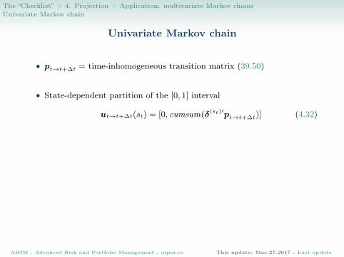
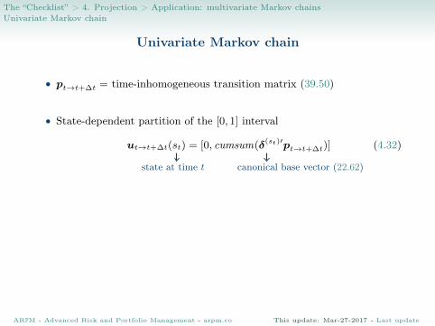
The “Checklist” > 4. Projection > Application: multivariate Markov chainsUnivariate Markov chain

Univariate Markov chain

• pt→t+∆t = time-inhomogeneous transition matrix (39.50)

• State-dependent partition of the [0, 1] interval

ut→t+∆t(st) = [0, cumsum(δ(st)′pt→t+∆t)] (4.32)

state at time t canonical base vector (22.62)

• Next-step function (4.8)

St+∆t = s|it ⇔ bucket(εt→t+∆t,ut→t+∆t(St)) = s (4.33)

shock ∼ Unif ([0, 1]) (4.34)

ARPM - Advanced Risk and Portfolio Management - arpm.co This update: Mar-27-2017 - Last update

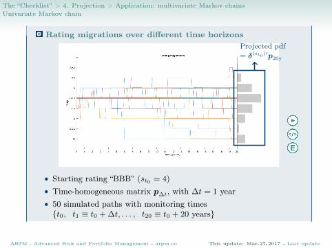
The “Checklist” > 4. Projection > Application: multivariate Markov chainsUnivariate Markov chain

Rating migrations over different time horizons

• Starting rating “BBB” (st0 = 4)• Time-homogeneous matrix p∆t, with ∆t = 1 year• 50 simulated paths with monitoring times{t0, t1 ≡ t0 + ∆t, . . . , t20 ≡ t0 + 20 years}

Projected pdf= δ(st0 )′p20y

ARPM - Advanced Risk and Portfolio Management - arpm.co This update: Mar-27-2017 - Last update

The “Checklist” > 4. Projection > Application: multivariate Markov chainsConnection with structural credit model

Connection with the Merton model

Next-step function for the Merton model (mirrors Section 2.3.5):

St+∆t = s|it ⇔ bucket(εt→t+∆t,ut→t+∆t(lt→t+∆t)) = s (4.35)

F losst→t+∆t(C

losst→t+∆t) ∼ Unif ([0, 1]) (4.36)

partition of [0, 1]: [0, . . . , ut→t+∆t(lt→t+∆t, s), . . . , 1]

F losst→t+∆t(−qlosst+∆t→t+2∆t(1− u(s))− ln(vliabt+2∆t/v

liabt+∆t)− lt→t+∆t) (4.37)

The shock in (4.36) can be expressed as

εt→t+∆t ≡ gt(−Cequityt→t+∆t) (4.38)

cdf of −Cequityt→t+∆t (⇒ increasing)

ARPM - Advanced Risk and Portfolio Management - arpm.co This update: Mar-27-2017 - Last update

The “Checklist” > 4. Projection > Application: multivariate Markov chainsConnection with structural credit model

Connection with the Merton model

Next-step function for the Merton model (mirrors Section 2.3.5):

St+∆t = s|it ⇔ bucket(εt→t+∆t,ut→t+∆t(lt→t+∆t)) = s (4.35)

F losst→t+∆t(C

losst→t+∆t) ∼ Unif ([0, 1]) (4.36)

partition of [0, 1]: [0, . . . , ut→t+∆t(lt→t+∆t, s), . . . , 1]

F losst→t+∆t(−qlosst+∆t→t+2∆t(1− u(s))− ln(vliabt+2∆t/v

liabt+∆t)− lt→t+∆t) (4.37)

The shock in (4.36) can be expressed as

εt→t+∆t ≡ gt(−Cequityt→t+∆t) (4.38)

cdf of −Cequityt→t+∆t (⇒ increasing)

ARPM - Advanced Risk and Portfolio Management - arpm.co This update: Mar-27-2017 - Last update

The “Checklist” > 4. Projection > Application: multivariate Markov chainsConnection with structural credit model

Connection with the Merton model

Next-step function for the Merton model (mirrors Section 2.3.5):

St+∆t = s|it ⇔ bucket(εt→t+∆t,ut→t+∆t(lt→t+∆t)) = s (4.35)

F losst→t+∆t(C

losst→t+∆t) ∼ Unif ([0, 1]) (4.36)

partition of [0, 1]: [0, . . . , ut→t+∆t(lt→t+∆t, s), . . . , 1]

F losst→t+∆t(−qlosst+∆t→t+2∆t(1− u(s))− ln(vliabt+2∆t/v

liabt+∆t)− lt→t+∆t) (4.37)

The shock in (4.36) can be expressed as

εt→t+∆t ≡ gt(−Cequityt→t+∆t) (4.38)

cdf of −Cequityt→t+∆t (⇒ increasing)

ARPM - Advanced Risk and Portfolio Management - arpm.co This update: Mar-27-2017 - Last update

The “Checklist” > 4. Projection > Application: multivariate Markov chainsConnection with structural credit model

Connection with the Merton model

Next-step function for the Merton model (mirrors Section 2.3.5):

St+∆t = s|it ⇔ bucket(εt→t+∆t,ut→t+∆t(lt→t+∆t)) = s (4.35)

F losst→t+∆t(C

losst→t+∆t) ∼ Unif ([0, 1]) (4.36)

partition of [0, 1]: [0, . . . , ut→t+∆t(lt→t+∆t, s), . . . , 1]

F losst→t+∆t(−qlosst+∆t→t+2∆t(1− u(s))− ln(vliabt+2∆t/v

liabt+∆t)− lt→t+∆t) (4.37)

The shock in (4.36) can be expressed as

εt→t+∆t ≡ gt(−Cequityt→t+∆t) (4.38)

cdf of −Cequityt→t+∆t (⇒ increasing)

ARPM - Advanced Risk and Portfolio Management - arpm.co This update: Mar-27-2017 - Last update

The “Checklist” > 4. Projection > Application: multivariate Markov chainsConnection with structural credit model

Connection with the Merton model

Next-step function for the Merton model (mirrors Section 2.3.5):

St+∆t = s|it ⇔ bucket(εt→t+∆t,ut→t+∆t(lt→t+∆t)) = s (4.35)

F losst→t+∆t(C

losst→t+∆t) ∼ Unif ([0, 1]) (4.36)

partition of [0, 1]: [0, . . . , ut→t+∆t(lt→t+∆t, s), . . . , 1]

F losst→t+∆t(−qlosst+∆t→t+2∆t(1− u(s))− ln(vliabt+2∆t/v

liabt+∆t)− lt→t+∆t) (4.37)

The shock in (4.36) can be expressed as

εt→t+∆t ≡ gt(−Cequityt→t+∆t) (4.38)

cdf of −Cequityt→t+∆t (⇒ increasing)

ARPM - Advanced Risk and Portfolio Management - arpm.co This update: Mar-27-2017 - Last update

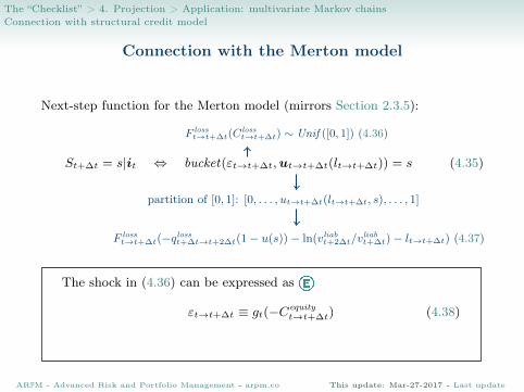
The “Checklist” > 4. Projection > Application: multivariate Markov chainsConnection with structural credit model

Connection with the Merton model

Next-step function for the Merton model (mirrors Section 2.3.5):

St+∆t = s|it ⇔ bucket(εt→t+∆t,ut→t+∆t(lt→t+∆t)) = s (4.35)

F losst→t+∆t(C

losst→t+∆t) ∼ Unif ([0, 1]) (4.36)

partition of [0, 1]: [0, . . . , ut→t+∆t(lt→t+∆t, s), . . . , 1]

F losst→t+∆t(−qlosst+∆t→t+2∆t(1− u(s))− ln(vliabt+2∆t/v

liabt+∆t)− lt→t+∆t) (4.37)

The shock in (4.36) can be expressed as

εt→t+∆t ≡ gt(−Cequityt→t+∆t) (4.38)

cdf of −Cequityt→t+∆t (⇒ increasing)

ARPM - Advanced Risk and Portfolio Management - arpm.co This update: Mar-27-2017 - Last update

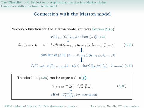
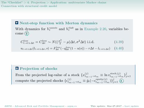
The “Checklist” > 4. Projection > Application: multivariate Markov chainsConnection with structural credit model

Next-step function with Merton dynamics

With dynamics for V assetst and V liab

t as in Example 2.20, variables be-come

C losst→t+∆t = C loss

∆t ∼ N ((σ2

2− µ)∆t, σ2∆t) i.i.d. (4.39)

ut→t+∆t(lt→t+∆t, s) = F loss∆t (−qloss∆t (1− u(s))− r∆t− lt→t+∆t) (4.40)

Projection of shocks

From the projected log-value of a stock {x(j)tm−1→tm ≡ ln v

stock ;(j)tm−1→tm}

jj=1

compute the projected shocks {ε(j)tm−1→tm ≡ gt(−cequity;(j)tm−1→tm)}jj=1

ARPM - Advanced Risk and Portfolio Management - arpm.co This update: Mar-27-2017 - Last update

The “Checklist” > 4. Projection > Application: multivariate Markov chainsMultivariate Markov Chains

Multivariate Markov Chains

• Risk drivers Xt ≡ (X1,t, . . . , Xd,t)′ with values

Xd,t ∈ {x(1), . . . , x(s), . . . , x(s)}, d = 1, . . . , d (4.41)

• Xd,t determined by state Sd,t ⇒ Xd,t = x(Sd,t)

• Next-step function for each d-th entry

Sd,tm = s|itm−1 ⇔ Sd,tm = bucket(εi,tm−1→tm ,utm−1→tm(Stm−1))

(4.42)• each entry Xd driven by one single shock εi ∼ Unif ([0, 1]) =⇒ ı = d

• {εd,tm−1→tm}dd=1 not independent as simultaneous variables

⇒ εtm−1→tm ≡

ε1,tm−1→tm

·εd,tm−1→tm

·εd,tm−1→tm

∼ Copε;m (4.44)

ARPM - Advanced Risk and Portfolio Management - arpm.co This update: Mar-27-2017 - Last update

The “Checklist” > 4. Projection > Application: multivariate Markov chainsMultivariate Markov Chains

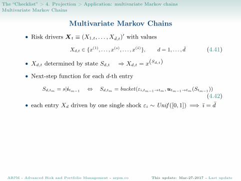
Multivariate Markov Chains

• Risk drivers Xt ≡ (X1,t, . . . , Xd,t)′ with values

Xd,t ∈ {x(1), . . . , x(s), . . . , x(s)}, d = 1, . . . , d (4.41)

• Xd,t determined by state Sd,t ⇒ Xd,t = x(Sd,t)

• Next-step function for each d-th entry

Sd,tm = s|itm−1 ⇔ Sd,tm = bucket(εi,tm−1→tm ,utm−1→tm(Stm−1))

(4.42)• each entry Xd driven by one single shock εi ∼ Unif ([0, 1]) =⇒ ı = d

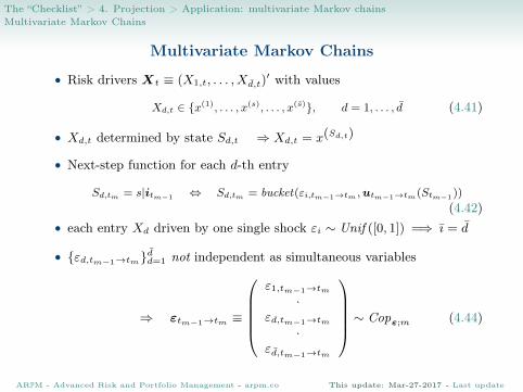
• {εd,tm−1→tm}dd=1 not independent as simultaneous variables

⇒ εtm−1→tm ≡

ε1,tm−1→tm

·εd,tm−1→tm

·εd,tm−1→tm

∼ Copε;m (4.44)

ARPM - Advanced Risk and Portfolio Management - arpm.co This update: Mar-27-2017 - Last update

The “Checklist” > 4. Projection > Application: multivariate Markov chainsMultivariate Markov Chains

Multivariate Markov Chains

• Risk drivers Xt ≡ (X1,t, . . . , Xd,t)′ with values

Xd,t ∈ {x(1), . . . , x(s), . . . , x(s)}, d = 1, . . . , d (4.41)

• Xd,t determined by state Sd,t ⇒ Xd,t = x(Sd,t)

• Next-step function for each d-th entry

Sd,tm = s|itm−1 ⇔ Sd,tm = bucket(εi,tm−1→tm ,utm−1→tm(Stm−1))

(4.42)

• each entry Xd driven by one single shock εi ∼ Unif ([0, 1]) =⇒ ı = d

• {εd,tm−1→tm}dd=1 not independent as simultaneous variables

⇒ εtm−1→tm ≡

ε1,tm−1→tm

·εd,tm−1→tm

·εd,tm−1→tm

∼ Copε;m (4.44)

ARPM - Advanced Risk and Portfolio Management - arpm.co This update: Mar-27-2017 - Last update

The “Checklist” > 4. Projection > Application: multivariate Markov chainsMultivariate Markov Chains

Multivariate Markov Chains

• Risk drivers Xt ≡ (X1,t, . . . , Xd,t)′ with values

Xd,t ∈ {x(1), . . . , x(s), . . . , x(s)}, d = 1, . . . , d (4.41)

• Xd,t determined by state Sd,t ⇒ Xd,t = x(Sd,t)

• Next-step function for each d-th entry

Sd,tm = s|itm−1 ⇔ Sd,tm = bucket(εi,tm−1→tm ,utm−1→tm(Stm−1))

(4.42)• each entry Xd driven by one single shock εi ∼ Unif ([0, 1]) =⇒ ı = d

• {εd,tm−1→tm}dd=1 not independent as simultaneous variables

⇒ εtm−1→tm ≡

ε1,tm−1→tm

·εd,tm−1→tm

·εd,tm−1→tm

∼ Copε;m (4.44)

ARPM - Advanced Risk and Portfolio Management - arpm.co This update: Mar-27-2017 - Last update

The “Checklist” > 4. Projection > Application: multivariate Markov chainsMultivariate Markov Chains

Multivariate Markov Chains

• Risk drivers Xt ≡ (X1,t, . . . , Xd,t)′ with values

Xd,t ∈ {x(1), . . . , x(s), . . . , x(s)}, d = 1, . . . , d (4.41)

• Xd,t determined by state Sd,t ⇒ Xd,t = x(Sd,t)

• Next-step function for each d-th entry

Sd,tm = s|itm−1 ⇔ Sd,tm = bucket(εi,tm−1→tm ,utm−1→tm(Stm−1))

(4.42)• each entry Xd driven by one single shock εi ∼ Unif ([0, 1]) =⇒ ı = d

• {εd,tm−1→tm}dd=1 not independent as simultaneous variables

⇒ εtm−1→tm ≡

ε1,tm−1→tm

·εd,tm−1→tm

·εd,tm−1→tm

∼ Copε;m (4.44)

ARPM - Advanced Risk and Portfolio Management - arpm.co This update: Mar-27-2017 - Last update

The “Checklist” > 4. Projection > Application: multivariate Markov chainsMultivariate Markov Chains

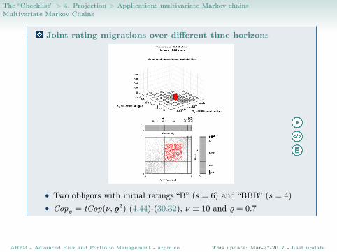
Joint rating migrations over different time horizons

• Two obligors with initial ratings “B” (s = 6) and “BBB” (s = 4)• Copε = tCop(ν,%2) (4.44)-(30.32), ν ≡ 10 and % = 0.7

ARPM - Advanced Risk and Portfolio Management - arpm.co This update: Mar-27-2017 - Last update

The “Checklist” > 4. Projection > Application: multivariate Markov chainsConnection with structural credit model

Merton model application

• Marginal d shocks in univariate case (4.35)

εd,tm−1→tm ≡ Flossd,tm−1→tm(C loss

d,tm−1→tm) ∼ Unif ([0, 1]) i.i.d. (4.45)

The shock in (4.36) can be expressed as

εd,tm−1→tm ≡ gd,m(−Cequityd,tm−1→tm) (4.46)

cdf of −Cequityd,tm−1→tm (⇒ increasing)

Copulas of εtm−1→tm and −Cequitytm−1→tm coincide

Copε;m

(30.4)≡ Cop−Cequity ;m

⇒ Correlation %2m can be estimated from the scenarios of −Cequity

Joint rating migrations with Merton model

ARPM - Advanced Risk and Portfolio Management - arpm.co This update: Mar-27-2017 - Last update

The “Checklist” > 4. Projection > Application: multivariate Markov chainsConnection with structural credit model

Merton model application

• Marginal d shocks in univariate case (4.35)

εd,tm−1→tm ≡ Flossd,tm−1→tm(C loss

d,tm−1→tm) ∼ Unif ([0, 1]) i.i.d. (4.45)

The shock in (4.36) can be expressed as

εd,tm−1→tm ≡ gd,m(−Cequityd,tm−1→tm) (4.46)

cdf of −Cequityd,tm−1→tm (⇒ increasing)

Copulas of εtm−1→tm and −Cequitytm−1→tm coincide

Copε;m

(30.4)≡ Cop−Cequity ;m

⇒ Correlation %2m can be estimated from the scenarios of −Cequity

Joint rating migrations with Merton model

ARPM - Advanced Risk and Portfolio Management - arpm.co This update: Mar-27-2017 - Last update

The “Checklist” > 4. Projection > Application: multivariate Markov chainsConnection with structural credit model

Merton model application

• Marginal d shocks in univariate case (4.35)

εd,tm−1→tm ≡ Flossd,tm−1→tm(C loss

d,tm−1→tm) ∼ Unif ([0, 1]) i.i.d. (4.45)

The shock in (4.36) can be expressed as

εd,tm−1→tm ≡ gd,m(−Cequityd,tm−1→tm) (4.46)

cdf of −Cequityd,tm−1→tm (⇒ increasing)

Copulas of εtm−1→tm and −Cequitytm−1→tm coincide

Copε;m

(30.4)≡ Cop−Cequity ;m

⇒ Correlation %2m can be estimated from the scenarios of −Cequity

Joint rating migrations with Merton model

ARPM - Advanced Risk and Portfolio Management - arpm.co This update: Mar-27-2017 - Last update

The “Checklist” > 4. Projection > Application: multivariate Markov chainsConnection with structural credit model

Merton model application

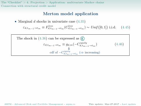
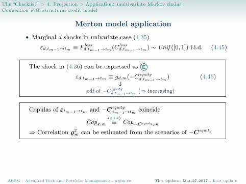
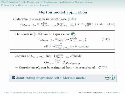
• Marginal d shocks in univariate case (4.35)

εd,tm−1→tm ≡ Flossd,tm−1→tm(C loss

d,tm−1→tm) ∼ Unif ([0, 1]) i.i.d. (4.45)

The shock in (4.36) can be expressed as

εd,tm−1→tm ≡ gd,m(−Cequityd,tm−1→tm) (4.46)

cdf of −Cequityd,tm−1→tm (⇒ increasing)

Copulas of εtm−1→tm and −Cequitytm−1→tm coincide

Copε;m

(30.4)≡ Cop−Cequity ;m

⇒ Correlation %2m can be estimated from the scenarios of −Cequity

Joint rating migrations with Merton model

ARPM - Advanced Risk and Portfolio Management - arpm.co This update: Mar-27-2017 - Last update

The “Checklist” > 4. Projection > Application: multivariate Markov chainsConnection with structural credit model

Merton model application

• Marginal d shocks in univariate case (4.35)

εd,tm−1→tm ≡ Flossd,tm−1→tm(C loss

d,tm−1→tm) ∼ Unif ([0, 1]) i.i.d. (4.45)

The shock in (4.36) can be expressed as

εd,tm−1→tm ≡ gd,m(−Cequityd,tm−1→tm) (4.46)

cdf of −Cequityd,tm−1→tm (⇒ increasing)

Copulas of εtm−1→tm and −Cequitytm−1→tm coincide

Copε;m

(30.4)≡ Cop−Cequity ;m

⇒ Correlation %2m can be estimated from the scenarios of −Cequity

Joint rating migrations with Merton model

ARPM - Advanced Risk and Portfolio Management - arpm.co This update: Mar-27-2017 - Last update