arX

iv:a

stro

-ph/

0611

642v

1 2

0 N

ov 2

006

ASTROPHYSICAL JOURNALPreprint typeset using LATEX style emulateapj v. 10/09/06

RELATIVISTIC BEAMING AND THE INTRINSIC PROPERTIES OF EXTRAGALACTIC RADIO JETS

M. H. COHEN1, M. L. L ISTER2, D. C. HOMAN3, M. KADLER4,5 K. I. K ELLERMANN6, Y. Y. KOVALEV 5,7,8, AND R. C. VERMEULEN9

(Received October 6, 2006; Revised November 15, 2006; Accepted November 16, 2006)

ABSTRACTRelations between the observed quantities for a beamed radio jet, apparent transverse speed and apparent

luminosity (βapp,L), and the intrinsic quantities, Lorentz factor and intrinsic luminosity (γ,Lo), are investigated.The inversion from measured to intrinsic values is not unique, but approximate limits toγ andLo can be foundusing probability arguments. Roughly half the sources in a flux density–limited, beamed sample have a valueof γ close to the measuredβapp. The methods are applied to observations of 119 AGN jets madewith theVLBA at 15 GHz during 1994–2002. The results strongly support the common relativistic beam model for anextragalactic radio jet. The (βapp,L) data are closely bounded by a theoretical envelope, anaspectcurve forγ = 32, Lo = 1025 W Hz−1. This gives limits to the maximum values ofγ andLo in the sample:γmax ≈ 32,andLo,max ∼ 1026 W Hz−1. No sources with both highβapp and lowL are observed. This is not the result ofselection effects due to the observing limits, which are fluxdensityS> 0.5 Jy, and angular velocityµ < 4 masyr−1. Many of the fastest quasars have a pattern Lorentz factorγp close to that of the beam,γb, but some ofthe slow quasars must haveγp ≪ γb. Three of the 10 galaxies in the sample have a superluminal feature, withspeeds up toβapp≈ 6. The others are at most mildly relativistic. The galaxies are not off–axis versions of thepowerful quasars, but Cygnus A might be an exception.Subject headings:BL Lacertae objects: general — galaxies: active — galaxies:individual: Cygnus A —

galaxies: jets — galaxies: statistics — quasars: general

1. INTRODUCTION

In recent years VLBI observations have provided many ac-curate values of the apparent luminosity,L, of compact radiojets, and the apparent transverse speed,βapp, of features (com-ponents) moving along the jets. These quantities are of con-siderable interest, but the intrinsic physical parameters, theLorentz factor,γ, and the intrinsic luminosity,Lo, are morefundamental. In this paper we first consider the “inversionproblem;” i.e., the estimation of intrinsic quantities from ob-served quantities. We then apply the results to data from alarge multi–epoch survey we have carried out with the VLBAat 15 GHz.

The inversion problem is discussed in §2–§4 with an ideal-ized relativistic beam, one that has the same vector velocityeverywhere, and contains a component moving with the beamvelocity. The jet emission is Doppler boosted, and Monte–Carlo simulations are used to estimate the probabilities asso-ciated with selecting a source: that of selecting (βapp,L) from agiven (γ,Lo); and the converse, the probability of (γ,Lo) beingthe intrinsic parameters for an observed (βapp,L).

1 Department of Astronomy, Mail Stop 105-24, California Institute ofTechnology, Pasadena, CA 91125, U.S.A.; mhc@astro.caltech.edu

2 Department of Physics, Purdue University, 525 Northwestern Avenue,West Lafayette, IN 47907, U.S.A.; mlister@physics.purdue.edu

3 Department of Physics and Astronomy, Denison University, Granville,OH 43023, U.S.A.; homand@denison.edu

4 Astrophysics Science Division, NASA Goddard SpaceFlight Center, Greenbelt Road, Greenbelt, MD 20771, USA;mkadler@milkyway.gsfc.nasa.gov

5 Max-Planck-Institut für Radioastronomie, Auf dem Hügel 69, 53121Bonn, Germany; ykovalev@mpifr-bonn.mpg.de

6 National Radio Astronomy Observatory, 520 Edgemont Road, Char-lottesville, VA 22903–2475, U.S.A.; kkellerm@nrao.edu

7 Astro Space Center of Lebedev Physical Institute, Profsoyuznaya 84/32,117997 Moscow, Russia;

8 Jansky Fellow, National Radio Astronomy Observatory, P.O.Box 2,Green Bank, WV 24944, U.S.A.;

9 ASTRON, Netherlands Foundation for Research in Astronomy,P.O. Box2, NL-7990 AA Dwingeloo, The Netherlands; rvermeulen@astron.nl

In §4 we introduce the concept of an “aspect” curve, definedas the track of a source on the (βapp,L) plane (the observationplane) asθ (angle to the line-of-sight, LOS) is varied; and an“origin” curve, defined as the set of values on the (γ,Lo) plane(the intrinsic plane) from which the observed source can beexpressed. These provide a ready way to understand the in-version problem, and illustrate the lack of a unique inversionfor a particular source. Probabilistic limits provide constraintson the intrinsic parameters for an individual source; but whenthe entire sample of sources is considered, more general com-ments can be made, as in §7.

The observational data are discussed in §5. They arefrom a 2–cm VLBA survey, and have been publishedin a series of papers: Kellermann et al. (1998, hereafterPaper I), Zensus et al. (2002, Paper II), Kellermann et al.(2004, Paper III), Kovalev et al. (2005, Paper IV), and E. Roset al. 2007, in preparation. This is a continuing survey and thespeeds are regularly updated using new data; in this paper weinclude results up to 2006 September 15. The analysis alsoincludes some results from the MOJAVE program, which isan extension of the 2–cm survey using a statistically completesample (Lister & Homan 2005). Prior to Paper III, the largestcompilation of internal motions was in Vermeulen & Cohen(1994, hereafter VC94), who tabulated the internal proper mo-tion, µ, for 66 AGN, andβapp for all but the two withouta redshift. The data came from many observers, using vari-ous wavelengths and different VLBI arrays, and consequentlywere inhomogeneous. The 2–cm data used here were ob-tained with the VLBA over the period 1994–2002, and com-prise “Excellent” or “Good” apparent speeds (Paper III) forcomponents in 119 sources. This is a substantial improvementover earlier data sets, and allows us to make statistical studieswhich previously have not been possible. Other recent sur-veys are reported by Jorstad et al. (2005, hereafter J05) withdata on 15 AGN at 43 GHz, Homan et al. (2001) with data on12 AGN at 15 and 22 GHz, and Piner et al. (2006) with data

2 Cohen et al.

on 77 AGN at 8 GHz.In some sources it is clear that the beam and pattern speeds

are different, and to discuss this we differentiate betweentheLorentz factor of the beam,γb, and that for the pattern,γp. Inmost of this paper, however, we assumeγb ≈ γp and drop thesubscripts. In §6 and §7 peak values for the distributions ofγandLo in the sample are discussed, and in §8 the low–velocityquasars and BL Lacs are discussed. It is likely that some ofthese have components whose pattern speed is significantlyless than the beam speed. The radio galaxies in our sampleare discussed in §9, and we show that most of them are nothigh–angle versions of the powerful quasars. Cygnus A maybe an exception, and we speculate that it contains a fast centraljet (a spine), with a slow outer sheath.

In this paper we use a cosmology withH0 =70 km s−1 Mpc−1, Ωm = 0.3, andΩΛ = 0.7.

2. RELATIVISTIC BEAMS

In this Section the standard relations for an ideal relativis-tic beam (e.g., Blandford & Königl 1979) are reviewed. Thebeam is characterized by its Lorentz factor,γ, intrinsic lumi-nosity, Lo, and angleθ to the line of sight. From these theDoppler factor,δ, the apparent transverse speed,βapp, and theapparent luminosity,L, can be calculated:

δ = γ−1(1−β cosθ)−1 , (1)

βapp=β sinθ

1−β cosθ, (2)

L = Loδn , (3)

whereβ = (1− γ−2)1/2 is the speed of the beam in the AGNframe (units ofc) andLo is the luminosity that would be mea-sured by an observer in the frame of the radiating material.The exponentn in equation 3 combines effects due to the Kcorrection and those due to Doppler boosting:n=α+ p, whereα is the spectral index (S∼ να) andp is the Doppler boost ex-ponent, discussed in §2.1.

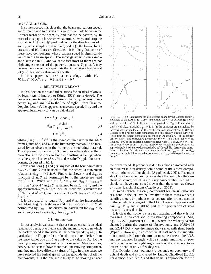
From equations (1) and (2), any two of the four parametersβapp, γ, δ, andθ can be used to find the others; a convenientrelation isβapp = βγδsinθ. Figure 1a showsδ andβapp asfunctions of sinθ, all normalized byγ; the curves are validfor γ2 ≫ 1. When sinθ = γ−1, δ = γ andβapp = βapp,max =βγ. The “critical” angleθc is defined by sinθc = γ−1, and theapproximationθ/θc ≈ γ sinθ will be used; this is accurate forγ2 ≫ 1 andθ2 ≪ 1, and is correct to 20% forθ < 60 andβ > 0.5.

It is also useful to regardβapp and θ as the independentquantities. Figure 1b showsδ andγ as functions of sinθ, allnormalized byβapp. The curves are calculated forβapp = 15and change slowly withβapp, for β2

app≫ 1.

2.1. Assumptions

In our analysis we assume that a source contains an idealrelativistic beam; one that is straight and narrow, and in whichthe pattern speed is the same as the beam speed:γp ≈ γb. Inparticular, the Doppler factor for the core must derive fromthe same values ofγ andθ as apply to the value ofβapp for themoving component, several pc or more away. Many sources,however, are seen to have more than one moving component,and they may have different values ofβapp. In these cases wehave selected the fastest speed, on the grounds that of all thecomponents, it is the one most likely to be moving at near

FIG. 1.— Top: Parameters for a relativistic beam having Lorentz factorγand angle to the LOSθ. (a) Curves are plotted forγ = 15 but change slowlywith γ, providedγ2 ≫ 1. (b) Curves are plotted forβapp = 15 and changeslowly with βapp, providedβ2

app≫ 1. In (a) the quantities are normalized bythe constant Lorentz factor; in (b), by the constant apparent speed.Bottom:Results from a Monte–Carlo simulation of a flux density–limited survey se-lected from the parent population described in Appendix A. (c) Probabilitydensityp(θ|γf ) and cumulative probabilityP(θ|γf) (heavy line) forγ ≈ 15.Roughly 75% of the selected sources will haveγ sinθ < 1; i.e.,θ < θc. Val-ues ofγ sinθ < 0.15 and> 2.0 are unlikely; the cumulative probabilities areapproximately 0.04 and 0.96, respectively. (d) Probability density and cumu-lative probability for selecting a source at angleθ, for βapp≈ 15. Asβappdecreases the probability curve becomes more peaked, and the peak moves tothe left.

the beam speed. It probably is due to a shock associated withan outburst in flux density, while some of the slower compo-nents might be trailing shocks (Agudo et al. 2001). The mainshock itself must be moving faster than the beam, but the syn-chrotron source, which is a density concentration behind theshock, can have a net speed slower than the shock, as shownby numerical simulations (Agudo et al. 2001).

In some sources the only component we see is stationaryat a bend in the jet. We believe that in these cases we see astanding shock, or perhaps enhanced radiation from a sectionof the jet which is tangent to the LOS. These components willhaveγp ≪ γb and might be part of the population of slowquasars discussed in §8.

It is clear that some jets are not straight, and thatθ is notthe same in the core and in the moving components. See,e.g., 3C 279 (Homan et al. 2003) where the velocity vectorchanged during the course of observations, and 0735+178and 2251+158, where the image shows a jet with sharp bends(Paper I). However, in cases where at least moderate superlu-minal motion is found, the motion must be close to the LOS,and any changes in angle will be strongly amplified by pro-jection. An observed right angle bend could correspond to anintrinsic bend of only a few degrees.

The Doppler boost exponentp depends on geometry andoptical depth and is discussed by Lind & Blandford (1985).For a smooth jet,p = 2, and this value is appropriate for the

Relativistic beaming in radio jets 3

core region, where, we assume, the relativistic beam streamsthrough a stationaryτ = 1 region. In some cases the mov-ing component can be modelled as an isolated optically thinsource, which would havep = 3, but for most of the sourcesthe flux density is dominated by radiation from the core, andwe usep= 2 here. See Figure 5 in Paper IV. The other term inthe exponentn is the spectral indexα. Nearly all the sourceshave a “flat" spectrum,|α| < 0.5, and they also have variableflux density and a variable spectrum. Because of the time de-pendence it is not possible to generate a useful index for eachsource, and we takeα = 0 as a rough global average, givingn = 2. This is further justified in §5.3, where it is shown thatn = 3 does not fit the data. However, this choice ofα = 0clearly leads to error for those sources with a high Dopplerfactor, sayδ = 30, because the K-correction must cover a fre-quency range of a factor of 30. This introduces uncertaintyinto the estimates of intrinsic luminosity.

We shall use equation (3) as ifLo is independent ofθ, butthis is not necessarily so. The opacity in the surrounding ma-terial may change withθ, and the luminosity of any opticallythick component may change with angle. Other changes inLomight be caused by a change in location of the emission re-gion, asθ, and therefore the Doppler factor and the emissionfrequency, change (Lobanov 1998).

3. PROBABILITY

The probability of selecting a source with a particular valueof θ, γ, βapp, or δ from a flux density–limited sample ofrelativistically–boosted sources is central to our discussion.BecauseS∝ δ2 (§5.3) andδ decreases with increasingθ,the sources found will preferentially be at small angles, eventhough there is not much solid angle there. VC94 calcu-lated the probabilityp(θ|γ f ) (the subscriptf meansfixed) ina Euclidean universe, and Lister & Marscher (1997, hereafterLM97) extended this with Monte–Carlo calculations, to in-clude evolution. However, the observations directly giveβapp,not γ, and p(θ|βapp,f) is generally not an analytic function.To deal with this, M. Lister et al. (in preparation) are usingMonte–Carlo methods to study the probability functions. Weuse one of their simulations here, as an illustrative example.

In the Monte–Carlo calculation, a simulated parent popu-lation is created (see Appendix A), from which one hundredthousand sources withS> 1.5 Jy are drawn. We select a sliceof this sample with 14.5≤ γ ≤ 15.5 and form the histogramsin Figure 1c, showing the probability densityp(θ|γf) and thecumulative probabilityP(θ|γf) for those sources withγ ≈ 15.The histograms vary slowly withγ, providedγ2 ≫ 1. Theyare similar to the equivalent diagrams calculated by VC94(Figure 7) and by LM97 (Figure 5). Figure 1c may be di-rectly compared with Figure 1a, which is a purely geometricresult from equations 1 and 2. The peak of the probabilityis at sinθ ≈ 0.6/γ, whereβapp ≈ 0.9γ and δ ≈ 1.5γ. The50% point ofP(θ|γf) is atγ sinθ≈ 0.7, giving a median valueθmed≈ 0.7γ−1 ≈ 0.7θc.

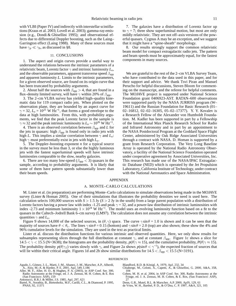
An interesting measure of the cumulative probability isP(θ = θc), the fraction of the sample lying inside the criticalangle. The slow variation of this fraction withγ is seen inFigure 2a; a rough value is 0.75; i.e., most beamed sourceswill be inside their “1/γ cones." In this paper we will take0.04< P< 0.96 as a practical range for the probability. Thiscorresponds, approximately, to 0.15< θ/θc < 2 for γ = 15,and the angular range for this probability range varies slowlywith γ. Figure 9 (Appendix A) shows the (γ,θ) distributionfor 14,000 sources from the simulation, along with the 4%

FIG. 2.— (a) Probability thatγ sinθ < 1 as a function ofγ. (b) (solidcurve) median value ofγ/βappand (dashed curve) median value ofβappsinθ,as functions ofβapp.

and 96% limits.We have now describedp(θ|γf), the probability for selecting

a jet at angleθ if it has Lorentz factorγ f . However, giventhat we observeβapp and notγ, we must consider also theprobability p(θ|βapp,f); i.e., the probability of finding a jet atthe angleθ if it has a fixedβapp. We again use a slice of theMonte–Carlo simulation, now for 14.5< βapp< 15.5, to getthe probabilities shown in Figure 1d. The probability densitycurve is broad, and asβappdecreases it becomes more peaked.The median value ofβappsinθ is shown with the dashed linein Figure 2b, as a function ofβapp.

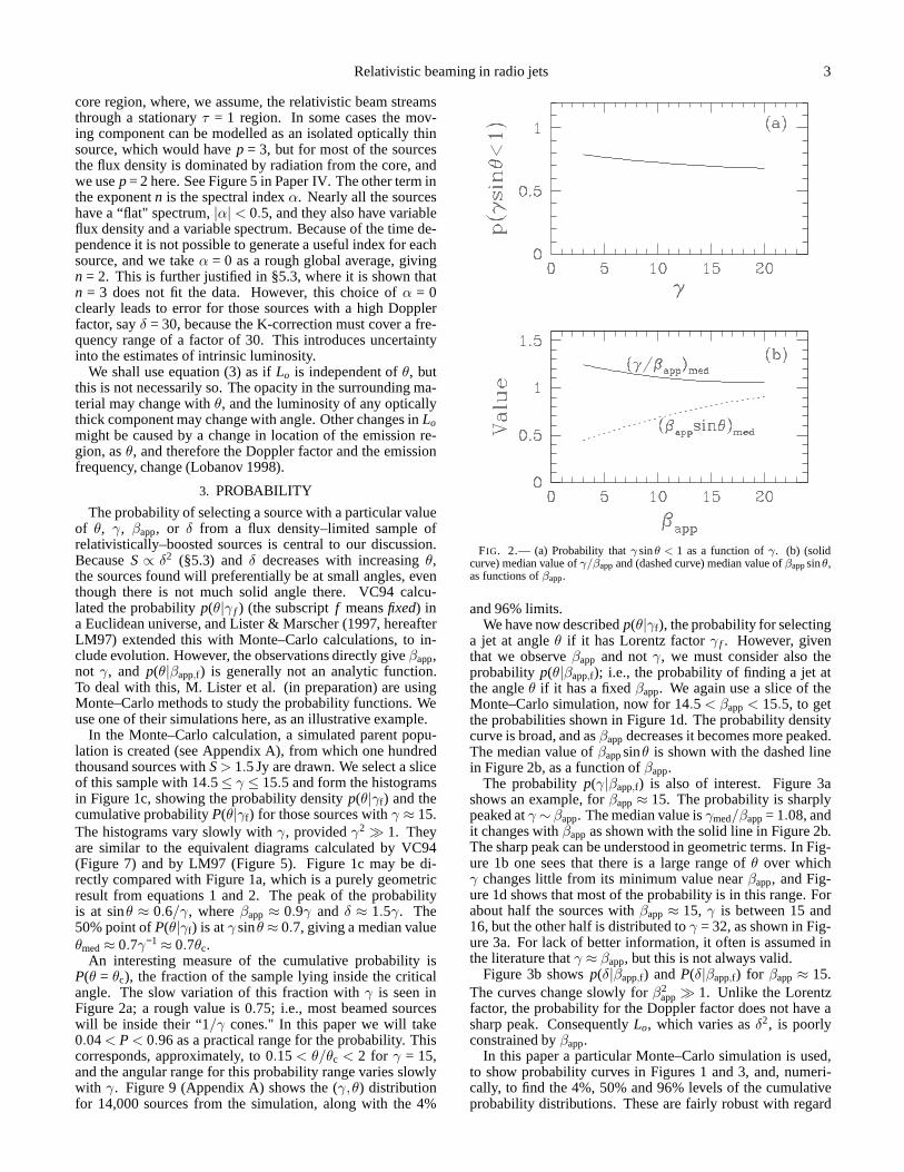
The probabilityp(γ|βapp,f) is also of interest. Figure 3ashows an example, forβapp≈ 15. The probability is sharplypeaked atγ ∼ βapp. The median value isγmed/βapp= 1.08, andit changes withβapp as shown with the solid line in Figure 2b.The sharp peak can be understood in geometric terms. In Fig-ure 1b one sees that there is a large range ofθ over whichγ changes little from its minimum value nearβapp, and Fig-ure 1d shows that most of the probability is in this range. Forabout half the sources withβapp ≈ 15, γ is between 15 and16, but the other half is distributed toγ = 32, as shown in Fig-ure 3a. For lack of better information, it often is assumed inthe literature thatγ ≈ βapp, but this is not always valid.

Figure 3b showsp(δ|βapp,f) andP(δ|βapp,f) for βapp ≈ 15.The curves change slowly forβ2

app≫ 1. Unlike the Lorentzfactor, the probability for the Doppler factor does not haveasharp peak. ConsequentlyLo, which varies asδ2, is poorlyconstrained byβapp.

In this paper a particular Monte–Carlo simulation is used,to show probability curves in Figures 1 and 3, and, numeri-cally, to find the 4%, 50% and 96% levels of the cumulativeprobability distributions. These are fairly robust with regard

4 Cohen et al.

FIG. 3.— Probability density and cumulative probability (heavy line) whenβapp≈ 15. (a)p(γ|βapp,f); (b) p(δ|βapp,f ).

to evolution and parent luminosity functions. We have com-pared them among several of the simulations calculated byM. Lister et al., and the variations are not enough to materi-ally affect any of the conclusions in this paper.

Figures 1–3 are not valid in the non–relativistic case, whereβ2 ≪ 1, γ ≈ 1, δ ≈ 1, βapp≈ β sinθ, and p(θ) ∼ sinθ. Ourdiscussion is also not valid for samples selected on the basisof non–beamed emission.

4. THE INVERSION PROBLEM

VLBA observations can directly give apparent speedβappand apparent luminosityL, but the Lorentz factorγ and theintrinsic luminosityLo are more useful. We refer to the esti-mation of the latter from the former as the inversion problem.

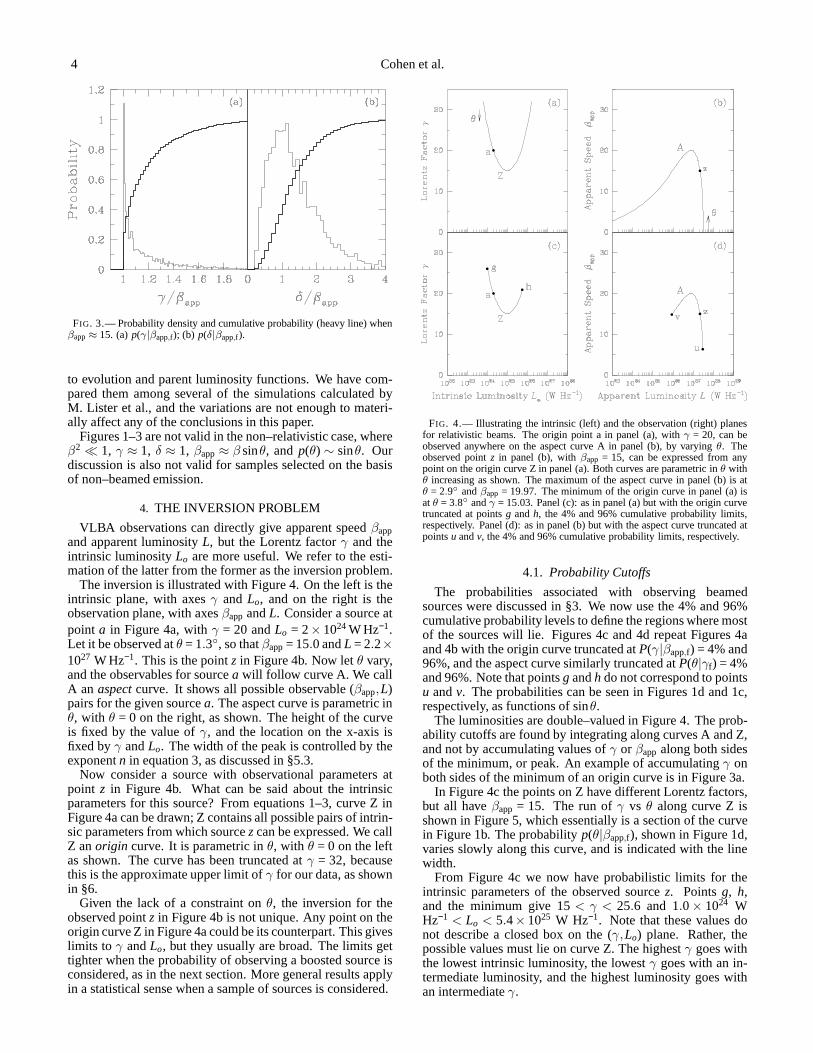
The inversion is illustrated with Figure 4. On the left is theintrinsic plane, with axesγ and Lo, and on the right is theobservation plane, with axesβapp andL. Consider a source atpoint a in Figure 4a, withγ = 20 andLo = 2× 1024W Hz−1.Let it be observed atθ = 1.3, so thatβapp= 15.0 andL = 2.2×1027 W Hz−1. This is the pointz in Figure 4b. Now letθ vary,and the observables for sourcea will follow curve A. We callA an aspectcurve. It shows all possible observable (βapp,L)pairs for the given sourcea. The aspect curve is parametric inθ, with θ = 0 on the right, as shown. The height of the curveis fixed by the value ofγ, and the location on the x-axis isfixed byγ andLo. The width of the peak is controlled by theexponentn in equation 3, as discussed in §5.3.

Now consider a source with observational parameters atpoint z in Figure 4b. What can be said about the intrinsicparameters for this source? From equations 1–3, curve Z inFigure 4a can be drawn; Z contains all possible pairs of intrin-sic parameters from which sourcezcan be expressed. We callZ anorigin curve. It is parametric inθ, with θ = 0 on the leftas shown. The curve has been truncated atγ = 32, becausethis is the approximate upper limit ofγ for our data, as shownin §6.

Given the lack of a constraint onθ, the inversion for theobserved pointz in Figure 4b is not unique. Any point on theorigin curve Z in Figure 4a could be its counterpart. This giveslimits to γ andLo, but they usually are broad. The limits gettighter when the probability of observing a boosted source isconsidered, as in the next section. More general results applyin a statistical sense when a sample of sources is considered.

FIG. 4.— Illustrating the intrinsic (left) and the observation(right) planesfor relativistic beams. The origin point a in panel (a), withγ = 20, can beobserved anywhere on the aspect curve A in panel (b), by varying θ. Theobserved pointz in panel (b), withβapp = 15, can be expressed from anypoint on the origin curve Z in panel (a). Both curves are parametric inθ withθ increasing as shown. The maximum of the aspect curve in panel(b) is atθ = 2.9 andβapp = 19.97. The minimum of the origin curve in panel (a) isatθ = 3.8 andγ = 15.03. Panel (c): as in panel (a) but with the origin curvetruncated at pointsg andh, the 4% and 96% cumulative probability limits,respectively. Panel (d): as in panel (b) but with the aspect curve truncated atpointsu andv, the 4% and 96% cumulative probability limits, respectively.

4.1. Probability Cutoffs

The probabilities associated with observing beamedsources were discussed in §3. We now use the 4% and 96%cumulative probability levels to define the regions where mostof the sources will lie. Figures 4c and 4d repeat Figures 4aand 4b with the origin curve truncated atP(γ|βapp,f) = 4% and96%, and the aspect curve similarly truncated atP(θ|γf) = 4%and 96%. Note that pointsg andh do not correspond to pointsu andv. The probabilities can be seen in Figures 1d and 1c,respectively, as functions of sinθ.

The luminosities are double–valued in Figure 4. The prob-ability cutoffs are found by integrating along curves A and Z,and not by accumulating values ofγ or βapp along both sidesof the minimum, or peak. An example of accumulatingγ onboth sides of the minimum of an origin curve is in Figure 3a.

In Figure 4c the points on Z have different Lorentz factors,but all haveβapp = 15. The run ofγ vs θ along curve Z isshown in Figure 5, which essentially is a section of the curvein Figure 1b. The probabilityp(θ|βapp,f), shown in Figure 1d,varies slowly along this curve, and is indicated with the linewidth.

From Figure 4c we now have probabilistic limits for theintrinsic parameters of the observed sourcez. Pointsg, h,and the minimum give 15< γ < 25.6 and 1.0× 1024 WHz−1 < Lo < 5.4× 1025 W Hz−1. Note that these values donot describe a closed box on the (γ,Lo) plane. Rather, thepossible values must lie on curve Z. The highestγ goes withthe lowest intrinsic luminosity, the lowestγ goes with an in-termediate luminosity, and the highest luminosity goes withan intermediateγ.

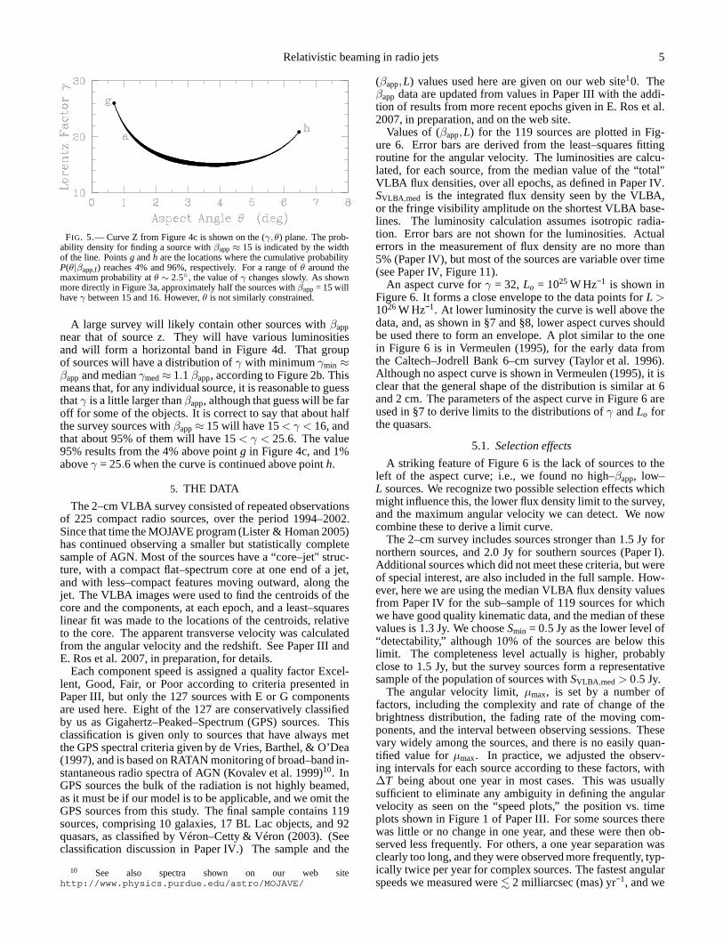
Relativistic beaming in radio jets 5

FIG. 5.— Curve Z from Figure 4c is shown on the (γ,θ) plane. The prob-ability density for finding a source withβapp≈ 15 is indicated by the widthof the line. Pointsg andh are the locations where the cumulative probabilityP(θ|βapp,f) reaches 4% and 96%, respectively. For a range ofθ around themaximum probability atθ ∼ 2.5, the value ofγ changes slowly. As shownmore directly in Figure 3a, approximately half the sources with βapp= 15 willhaveγ between 15 and 16. However,θ is not similarly constrained.

A large survey will likely contain other sources withβappnear that of sourcez. They will have various luminositiesand will form a horizontal band in Figure 4d. That groupof sources will have a distribution ofγ with minimumγmin ≈βappand medianγmed≈ 1.1βapp, according to Figure 2b. Thismeans that, for any individual source, it is reasonable to guessthatγ is a little larger thanβapp, although that guess will be faroff for some of the objects. It is correct to say that about halfthe survey sources withβapp≈ 15 will have 15< γ < 16, andthat about 95% of them will have 15< γ < 25.6. The value95% results from the 4% above pointg in Figure 4c, and 1%aboveγ = 25.6 when the curve is continued above pointh.

5. THE DATA

The 2–cm VLBA survey consisted of repeated observationsof 225 compact radio sources, over the period 1994–2002.Since that time the MOJAVE program (Lister & Homan 2005)has continued observing a smaller but statistically completesample of AGN. Most of the sources have a “core–jet" struc-ture, with a compact flat–spectrum core at one end of a jet,and with less–compact features moving outward, along thejet. The VLBA images were used to find the centroids of thecore and the components, at each epoch, and a least–squareslinear fit was made to the locations of the centroids, relativeto the core. The apparent transverse velocity was calculatedfrom the angular velocity and the redshift. See Paper III andE. Ros et al. 2007, in preparation, for details.

Each component speed is assigned a quality factor Excel-lent, Good, Fair, or Poor according to criteria presented inPaper III, but only the 127 sources with E or G componentsare used here. Eight of the 127 are conservatively classifiedby us as Gigahertz–Peaked–Spectrum (GPS) sources. Thisclassification is given only to sources that have always metthe GPS spectral criteria given by de Vries, Barthel, & O’Dea(1997), and is based on RATAN monitoring of broad–band in-stantaneous radio spectra of AGN (Kovalev et al. 1999)10. InGPS sources the bulk of the radiation is not highly beamed,as it must be if our model is to be applicable, and we omit theGPS sources from this study. The final sample contains 119sources, comprising 10 galaxies, 17 BL Lac objects, and 92quasars, as classified by Véron–Cetty & Véron (2003). (Seeclassification discussion in Paper IV.) The sample and the

10 See also spectra shown on our web sitehttp://www.physics.purdue.edu/astro/MOJAVE/

(βapp,L) values used here are given on our web site10. Theβapp data are updated from values in Paper III with the addi-tion of results from more recent epochs given in E. Ros et al.2007, in preparation, and on the web site.

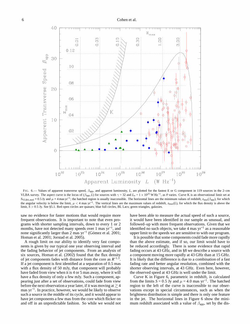
Values of (βapp,L) for the 119 sources are plotted in Fig-ure 6. Error bars are derived from the least–squares fittingroutine for the angular velocity. The luminosities are calcu-lated, for each source, from the median value of the “total"VLBA flux densities, over all epochs, as defined in Paper IV.SVLBA ,med is the integrated flux density seen by the VLBA,or the fringe visibility amplitude on the shortest VLBA base-lines. The luminosity calculation assumes isotropic radia-tion. Error bars are not shown for the luminosities. Actualerrors in the measurement of flux density are no more than5% (Paper IV), but most of the sources are variable over time(see Paper IV, Figure 11).

An aspect curve forγ = 32, Lo = 1025 W Hz−1 is shown inFigure 6. It forms a close envelope to the data points forL >1026 W Hz−1. At lower luminosity the curve is well above thedata, and, as shown in §7 and §8, lower aspect curves shouldbe used there to form an envelope. A plot similar to the onein Figure 6 is in Vermeulen (1995), for the early data fromthe Caltech–Jodrell Bank 6–cm survey (Taylor et al. 1996).Although no aspect curve is shown in Vermeulen (1995), it isclear that the general shape of the distribution is similar at 6and 2 cm. The parameters of the aspect curve in Figure 6 areused in §7 to derive limits to the distributions ofγ andLo forthe quasars.

5.1. Selection effects

A striking feature of Figure 6 is the lack of sources to theleft of the aspect curve; i.e., we found no high–βapp, low–L sources. We recognize two possible selection effects whichmight influence this, the lower flux density limit to the survey,and the maximum angular velocity we can detect. We nowcombine these to derive a limit curve.

The 2–cm survey includes sources stronger than 1.5 Jy fornorthern sources, and 2.0 Jy for southern sources (Paper I).Additional sources which did not meet these criteria, but wereof special interest, are also included in the full sample. How-ever, here we are using the median VLBA flux density valuesfrom Paper IV for the sub–sample of 119 sources for whichwe have good quality kinematic data, and the median of thesevalues is 1.3 Jy. We chooseSmin = 0.5 Jy as the lower level of“detectability,” although 10% of the sources are below thislimit. The completeness level actually is higher, probablyclose to 1.5 Jy, but the survey sources form a representativesample of the population of sources withSVLBA ,med> 0.5 Jy.

The angular velocity limit,µmax, is set by a number offactors, including the complexity and rate of change of thebrightness distribution, the fading rate of the moving com-ponents, and the interval between observing sessions. Thesevary widely among the sources, and there is no easily quan-tified value forµmax. In practice, we adjusted the observ-ing intervals for each source according to these factors, with∆T being about one year in most cases. This was usuallysufficient to eliminate any ambiguity in defining the angularvelocity as seen on the “speed plots,” the position vs. timeplots shown in Figure 1 of Paper III. For some sources therewas little or no change in one year, and these were then ob-served less frequently. For others, a one year separation wasclearly too long, and they were observed more frequently, typ-ically twice per year for complex sources. The fastest angularspeeds we measured were. 2 milliarcsec (mas) yr−1, and we

6 Cohen et al.

FIG. 6.— Values of apparent transverse speed,βapp, and apparent luminosity,L, are plotted for the fastest E or G component in 119 sources inthe 2–cmVLBA survey. The aspect curve is the locus of (βapp,L) for sources withγ = 32 andLo = 1×1025 W Hz−1, asθ varies. Curve K is an observational limit set atSVLBA ,med = 0.5 Jy andµ = 4 mas yr−1; the hatched region is usually inaccessible. The horizontal lines are the minimum values of redshift,zmin(βapp), for whichthe angular velocity is below the limit,µ < 4 mas yr−1. The vertical lines are the maximum values of redshift,zmax(L), for which the flux density is above thelimit, S> 0.5 Jy. See §5.1. Red open circles are quasars; blue full circles, BL Lacs; green triangles, galaxies.

saw no evidence for faster motions that would require morefrequent observations. It is important to note that even pro-grams with shorter sampling intervals, down to every 1 or 2months, have not detected many speeds over 1 mas yr−1, andnone significantly larger than 2 mas yr−1 (Gómez et al. 2001;Homan et al. 2001; Jorstad et al. 2005).

A rough limit on our ability to identify very fast compo-nents is given by our typical one year observing interval andthe fading behavior of jet components. From an analysis ofsix sources, Homan et al. (2002) found that the flux densityof jet components fades with distance from the core asR−1.3.If a jet component is first identified at a separation of 0.5 maswith a flux density of 50 mJy, that component will probablyhave faded from view when it is 4 or 5 mas away, where it willhave a flux density of only a few mJy. Such a component, ap-pearing just after a set of observations, could fade from viewbefore the next observation a year later, if it was moving at& 4mas yr−1. In practice, however, we would be likely to observesuch a source in the middle of its cycle, and it would appear tohave jet components a few mas from the core which flicker onand off in an unpredictable fashion. So while we would not

have been able to measure the actual speed of such a source,it would have been identified in our sample as unusual, andfollowed–up with more frequent observations. Given that weidentified no such objects, we take 4 mas yr−1 as a reasonableupper limit to the speeds we are sensitive to with our program.

It is possible that some components could fade more rapidlythan the above estimate, and if so, our limit would have tobe reduced accordingly. There is some evidence that rapidfading occurs at 43 GHz, and in §8 we describe a source witha component moving more rapidly at 43 GHz than at 15 GHz.It is likely that the difference is due to a combination of a fastfading rate and better angular resolution, combined with theshorter observing intervals, at 43 GHz. Even here, however,the observed speed at 43 GHz is well under the limit.

Curve K in Figure 6, parametric in redshift, is calculatedfrom the limitsS= 0.5 Jy andµ = 4.0 mas yr−1. The hatchedregion to the left of the curve is inaccessible to our obser-vations except in special circumstances, such as when thebrightness distribution is simple and there is only one featurein the jet. The horizontal lines in Figure 6 show the mini-mum redshift associated with a value ofβapp, set by the dis-

Relativistic beaming in radio jets 7

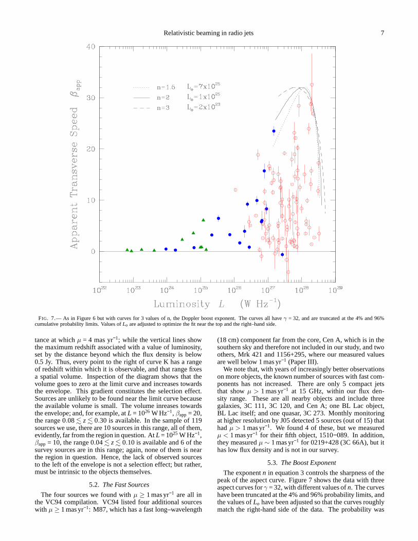
FIG. 7.— As in Figure 6 but with curves for 3 values of n, the Doppler boost exponent. The curves all haveγ = 32, and are truncated at the 4% and 96%cumulative probability limits. Values ofLo are adjusted to optimize the fit near the top and the right–hand side.

tance at whichµ = 4 mas yr−1; while the vertical lines showthe maximum redshift associated with a value of luminosity,set by the distance beyond which the flux density is below0.5 Jy. Thus, every point to the right of curve K has a rangeof redshift within which it is observable, and that range fixesa spatial volume. Inspection of the diagram shows that thevolume goes to zero at the limit curve and increases towardsthe envelope. This gradient constitutes the selection effect.Sources are unlikely to be found near the limit curve becausethe available volume is small. The volume inreases towardsthe envelope; and, for example, atL = 1026 W Hz−1, βapp= 20,the range 0.08. z. 0.30 is available. In the sample of 119sources we use, there are 10 sources in this range, all of them,evidently, far from the region in question. AtL = 1025 W Hz−1,βapp = 10, the range 0.04. z. 0.10 is available and 6 of thesurvey sources are in this range; again, none of them is nearthe region in question. Hence, the lack of observed sourcesto the left of the envelope is not a selection effect; but rather,must be intrinsic to the objects themselves.

5.2. The Fast Sources

The four sources we found withµ ≥ 1 mas yr−1 are all inthe VC94 compilation. VC94 listed four additional sourceswith µ ≥ 1 mas yr−1: M87, which has a fast long–wavelength

(18 cm) component far from the core, Cen A, which is in thesouthern sky and therefore not included in our study, and twoothers, Mrk 421 and 1156+295, where our measured valuesare well below 1 mas yr−1 (Paper III).

We note that, with years of increasingly better observationson more objects, the known number of sources with fast com-ponents has not increased. There are only 5 compact jetsthat showµ > 1 mas yr−1 at 15 GHz, within our flux den-sity range. These are all nearby objects and include threegalaxies, 3C 111, 3C 120, and Cen A; one BL Lac object,BL Lac itself; and one quasar, 3C 273. Monthly monitoringat higher resolution by J05 detected 5 sources (out of 15) thathadµ > 1 mas yr−1. We found 4 of these, but we measuredµ < 1 mas yr−1 for their fifth object, 1510−089. In addition,they measuredµ∼ 1 mas yr−1 for 0219+428 (3C 66A), but ithas low flux density and is not in our survey.

5.3. The Boost Exponent

The exponentn in equation 3 controls the sharpness of thepeak of the aspect curve. Figure 7 shows the data with threeaspect curves forγ = 32, with different values ofn. The curveshave been truncated at the 4% and 96% probability limits, andthe values ofLo have been adjusted so that the curves roughlymatch the right-hand side of the data. The probability was

8 Cohen et al.

calculated with equation (A15) from VC94, as the simulationdescribed in Appendix A usesn = 2 and has not been calcu-lated for other values ofn.

It is important to compare the curves with the data only inthe region where the probability is significant. From Figure7there is no strong reason to pick one value ofn over another.However, ifn = 3, the boosting becomes so strong that strongdistant quasars, near the peak of the distribution, haveLo assmall as the jets in weak nearby galaxies, which (we arguein §9) are only mildly relativistic. This is unrealistic, and weconclude thatn < 3. The valuen = 2 has a theoretical ba-sis (§2.1) and we have adopted it here. Note the large rangein intrinsic luminosity corresponding to different valuesof n.Sincen is not known with precision, the intrinsic luminositieshave a corresponding uncertainty.

6. THE PEAK LORENTZ FACTOR

Beaming is a powerful relativistic effect that supplies astrong selection mechanism in high–frequency observationsof AGN. Consider a sample of randomly oriented, relativis-tically boosted sources that have distributions in redshift, in-trinsic luminosity, and Lorentz factor. Make a flux density–limited survey of this sample. VC94 and LM97 have shownthat in this case the selected sources will have a maximumvalue ofβapp which closely approaches the upper limit of theγ distribution, even for rather small sample size. This comesabout because the probability of selecting a source is maxi-mized nearθ = 0.6θc whereβapp≈ 0.9γ (see Figure 1c); andthere is a high probability that, in a group of sources, somewill be at angles close toθc, whereβapp ≈ γ. Hence, be-causeβapp,max ≈ 32, the upper limit of theγ–distribution isγapp,max≈ 32.

7. THE DISTRIBUTIONS OFγ AND LO

We showed in §5.1 that the lack of sources to the left of theenvelope is not a selection effect, but is intrinsic to the ob-jects. Since the envelope is narrow at the top,βapp andL arecorrelated; highβapp is found only in sources that also havehigh L, but lowβapp is found in sources with all values ofL.This translates intoγ having a similar correlation withLo, forthe quasars. Theγ distribution will be similar to theβapp dis-tribution in Figure 7, but flatter; with many points shifted up,but nearly all by less than a factor 2 aboveβapp. TheLo dis-tribution will remain more spread out at lowγ than at highγ,leading to the correlation that the highestγ are found only injets with high intrinsic luminosity. This is consistent with aresult from LM97, that Monte–Carlo simulations with nega-tive correlation betweenγ andLo give a poor fit to the statis-tics of the flux densities from the Caltech–Jodrell Bank survey(Taylor et al. 1996).

The good fit of an aspect curve as an envelope to the datain Figure 6 suggests that the parameters of the curve,γ = 32andLo = 1025 W Hz−1, reflect the peak values ofγ andLo inthe population. The distribution ofγ may be a power law, assuggested by LM97 and, as discussed in §6,γmax = 32 is closeto the maximum value in the distribution. We now considerconstraints on the peak value forLo.

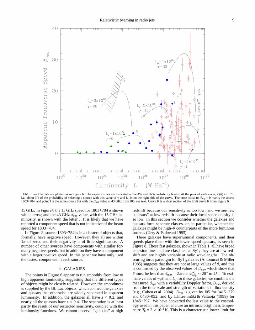
Figure 8 is similar to Figure 6, but with several aspectcurves, each showing only the region 0.04< P(θ|γf) < 0.96.The envelope is now formed by a series of aspect curves,with successively lower values ofγ. Most of the sources willhaveγ rather close toβapp, but some will haveγ substan-tially greater (see Figures 2b and 3a). In Figure 8 these lattersources will not lie near the top of an aspect curve, but will

be down from the peak. It is more likely that they will be atsmall angles (θ < θc) than at large angles.

Consider the BL Lac marked B, near the intersection ofcurvesγ = 6 andγ = 20. It could be on either curve, but itis near the low–probability region of curveγ = 20. For ev-ery source on curveγ = 20 near the intersection, there shouldbe several farther up the curve. Note that theγ = 20 curveintersects the limit curve K to the left of the peak. There islittle available redshift volume at the peak, but the volumein-creases rapidly at lowerβapp, and the lack of sources theremeans that source B is unlikely to haveγ = 20. Alternatively,it could be close to an extension of curveγ = 15, but then itis again in a low–probability region. There are a number ofsources near the peak of curveγ = 15, and B could be a high–angle version of one of them. But the probability of that iswell below 0.04, and there can be few such sources in the en-tire sample of 119. We conclude that the galaxies and BL Lacson the left side of the distribution (L< 3×1025W Hz−1), withhigh confidence, are not off-axis versions of the powerfulquasars (curvesγ = 15 and 32), nor are they high–γ, low–Losources (curveγ = 20).

Source B in Figure 8 is the eponymous object BL Lac,2200+420. Denn, Mutel & Marscher (2000) studied BL Lacin detail, and showed that the jet lies on a helix with axisθ = 9 and pitch angle 2. If θ = 9 ± 2 is combined withour value for the apparent transverse speed,βapp = 6.6±0.6,thenγ = 7±1. This agrees with our conclusion above.

Now consider the sources near point C in Figure 8, atL = 3×1028W Hz−1,βapp = 9. They could haveγ ≈ 9, but inthat case there should be several others down theγ = 9 curveto the right, where most of the probability lies. But there arenone there. Any aspect curve with a peak farther to the right isunlikely to represent any of the measured points, and so curveγ = 9 is about as far to the right as should be considered. If thesources at C are on curveγ = 9, then their intrinsic luminos-ity is an order of magnitude greater than that for the sourcesnear the top of the distribution, the fastest quasars. To avoida negative correlation betweenγ andLo, some of the sourcesnear point C should haveγ = 20 or more, with the appropriatesmall values ofθ. However, others near the right-hand side ofthe distribution might well haveγ ∼ 9 or smaller. This meansthat the distribution ofLo could extend up to 1026 W Hz−1.

8. QUASARS AND BL LACS WITHβAPP< 3

Twenty-two of the 92 quasars and 3 of the 13 powerfulBL Lacs in Figure 8 (L> 3×1025 W Hz−1) haveβapp< 3, andhave low probability ifγ > 10. What are the intrinsic proper-ties of this group? We consider three possibilities. (i) They arehigh–γ sources seen nearly end-on, and haveP(θ)< 0.04. Weexpect only a few such end-on sources out of a group of 105.Most of the low–speed quasars cannot be explained this way.(ii) They are low–γ high–Lo sources, and haveγ ∼ 3. We dis-cussed this above for point C in Figure 8 withβapp = 9; nowwe are consideringβapp < 3, and the argument is stronger.Unless the most intrinsically luminous sources have lowγ,this option is not viable. (iii) A more likely situation is thatmany of these low–βapp components appear to be slow be-causeγp < γb.

In support of comment (iii), we note that one of the slowobjects, 1803+784, was also observed by J05 at 43 GHz.They findβapp = 15.9± 1.9, whereas, at 15 GHz, we foundβapp = −0.6±0.6. The higher resolution at 43 GHz is crucialin detecting fast components in sources like this, because theyare within 1 mas of the core, at or below the resolution limit at

Relativistic beaming in radio jets 9

FIG. 8.— The data are plotted as in Figure 6. The aspect curves aretruncated at the 4% and 96% probability levels. At the peak ofeach curve,P(θ) ≈ 0.75;i.e. about 3/4 of the probability of selecting a source with this value ofγ andLo is on the right side of the curve. The cross close toβapp = 0 marks the source1803+784, and point J is the same source but with theβapp value at 43 GHz from J05, see text. Curve K is a short section ofthe limit curve K from Figure 6.

15 GHz. In Figure 8 the 15 GHz speed for 1803+784 is shownwith a cross; and the 43 GHzβapp value, with the 15 GHz lu-minosity, is shown with the letter J. It is likely that we havereported a component speed that is not indicative of the beamspeed for 1803+784.

In Figure 8, source 1803+784 is in a cluster of objects that,formally, have negative speed. However, they all are within1σ of zero, and their negativity is of little significance. Anumber of other sources have components with similar for-mally negative speeds, but in addition they have a componentwith a larger positive speed. In this paper we have only usedthe fastest component in each source.

9. GALAXIES

The points in Figure 6 appear to run smoothly from low tohigh apparent luminosity, suggesting that the different typesof objects might be closely related. However, the smoothnessis supplied by the BL Lac objects, which connect the galaxiesand quasars that otherwise are widely separated in apparentluminosity. In addition, the galaxies all havez ≤ 0.2, andnearly all the quasars havez> 0.4. The separation is at leastpartly the result of our restricted sensitivity, coupled with theluminosity functions. We cannot observe “galaxies” at high

redshift because our sensitivity is too low; and we see few“quasars” at low redshift because their local space densityisso low. In this section we consider whether the galaxies andquasars form separate classes, or, in particular, whether thegalaxies might be high–θ counterparts of the more luminoussources (Urry & Padovani 1995).

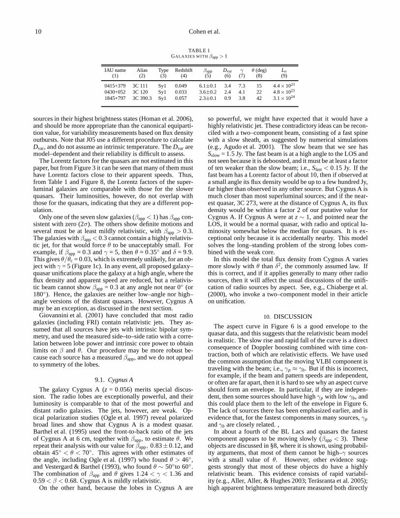
Three galaxies have superluminal components, and theirspeeds place them with the lower–speed quasars, as seen inFigure 8. These fast galaxies, shown in Table 1, all have broademission lines and are classified as Sy1; they are at low red-shift and are highly variable at radio wavelengths. The ob-scuring torus paradigm for Sy1 galaxies (Antonucci & Miller1985) suggests that they are not at large values ofθ, and thisis confirmed by the observed values ofβapp, which show thatθ must be less thanθmax = 2arctanβ−1

app∼ 20 to 45. To esti-mate values ofγ,θ, andLo for these galaxies, we combine themeasuredβapp with a variability Doppler factor,Dvar, derivedfrom the time scale and strength of variations in flux density(e.g., Cohen et al. 2004).Dvar is given by J05 for 0415+379and 0430+052, and by Lähteenmäki & Valtaoja (1999) for1845+797. We have converted the last value to the cosmol-ogy used in this paper, and use an intrinsic brightness temper-atureTb = 2× 1011K. This is a characteristic lower limit for

10 Cohen et al.

TABLE 1GALAXIES WITH βapp> 1

IAU name Alias Type Redshift βapp Dvar γ θ (deg) Lo(1) (2) (3) (4) (5) (6) (7) (8) (9)

0415+379 3C 111 Sy1 0.049 6.1±0.1 3.4 7.3 15 4.4×1023

0430+052 3C 120 Sy1 0.033 3.6±0.2 2.4 4.1 22 4.8×1023

1845+797 3C 390.3 Sy1 0.057 2.3±0.1 0.9 3.8 42 3.1×1024

sources in their highest brightness states (Homan et al. 2006),and should be more appropriate than the canonical equiparti-tion value, for variability measurements based on flux densityoutbursts. Note that J05 use a different procedure to calculateDvar, and do not assume an intrinsic temperature. TheDvar aremodel–dependent and their reliability is difficult to assess.

The Lorentz factors for the quasars are not estimated in thispaper, but from Figure 3 it can be seen that many of them musthave Lorentz factors close to their apparent speeds. Thus,from Table 1 and Figure 8, the Lorentz factors of the super-luminal galaxies are comparable with those for the slowerquasars. Their luminosities, however, do not overlap withthose for the quasars, indicating that they are a different pop-ulation.

Only one of the seven slow galaxies (βapp< 1) hasβappcon-sistent with zero (2σ). The others show definite motions andseveral must be at least mildly relativistic, withβapp > 0.3.The galaxies withβapp< 0.3 cannot contain a highly relativis-tic jet, for that would forceθ to be unacceptably small. Forexample, ifβapp = 0.3 andγ = 5, thenθ = 0.35 andδ = 9.9.This givesθ/θc = 0.03, which is extremely unlikely, for an ob-ject withγ = 5 (Figure 1c). In any event, all proposed galaxy–quasar unifications place the galaxy at a high angle, where theflux density and apparent speed are reduced, but a relativis-tic beam cannot showβapp = 0.3 at any angle not near 0 (or180). Hence, the galaxies are neither low–angle nor high–angle versions of the distant quasars. However, Cygnus Amay be an exception, as discussed in the next section.

Giovannini et al. (2001) have concluded that most radiogalaxies (including FRI) contain relativistic jets. They as-sumed that all sources have jets with intrinsic bipolar sym-metry, and used the measured side–to–side ratio with a corre-lation between lobe power and intrinsic core power to obtainlimits on β and θ. Our procedure may be more robust be-cause each source has a measuredβapp, and we do not appealto symmetry of the lobes.

9.1. Cygnus A

The galaxy Cygnus A (z = 0.056) merits special discus-sion. The radio lobes are exceptionally powerful, and theirluminosity is comparable to that of the most powerful anddistant radio galaxies. The jets, however, are weak. Op-tical polarization studies (Ogle et al. 1997) reveal polarizedbroad lines and show that Cygnus A is a modest quasar.Barthel et al. (1995) used the front-to-back ratio of the jetsof Cygnus A at 6 cm, together withβapp, to estimateθ. Werepeat their analysis with our value forβapp, 0.83±0.12, andobtain 45 < θ < 70. This agrees with other estimates ofthe angle, including Ogle et al. (1997) who foundθ > 46,and Vestergard & Barthel (1993), who foundθ ∼ 50to 60.The combination ofβapp and θ gives 1.24< γ < 1.36 and0.59< β < 0.68. Cygnus A is mildly relativistic.

On the other hand, because the lobes in Cygnus A are

so powerful, we might have expected that it would have ahighly relativistic jet. These contradictory ideas can be recon-ciled with a two–component beam, consisting of a fast spinewith a slow sheath, as suggested by numerical simulations(e.g., Agudo et al. 2001). The slow beam that we see hasSslow = 1.5 Jy. The fast beam is at a high angle to the LOS andnot seen because it is deboosted, and it must be at least a factorof ten weaker than the slow beam; i.e.,Sfast< 0.15 Jy. If thefast beam has a Lorentz factor of about 10, then if observed ata small angle its flux density would be up to a few hundred Jy,far higher than observed in any other source. But Cygnus A ismuch closer than most superluminal sources; and if the near-est quasar, 3C 273, were at the distance of Cygnus A, its fluxdensity would be within a factor 2 of our putative value forCygnus A. If Cygnus A were atz∼ 1, and pointed near theLOS, it would be a normal quasar, with radio and optical lu-minosity somewhat below the median for quasars. It is ex-ceptional only because it is accidentally nearby. This modelsolves the long–standing problem of the strong lobes com-bined with the weak core.

In this model the total flux density from Cygnus A variesmore slowly withθ thanδ2, the commonly assumed law. Ifthis is correct, and if it applies generally to many other radiosources, then it will affect the usual discussions of the unifi-cation of radio sources by aspect. See, e.g., Chiaberge et al.(2000), who invoke a two–component model in their articleon unification.

10. DISCUSSION

The aspect curve in Figure 6 is a good envelope to thequasar data, and this suggests that the relativistic beam modelis realistic. The slow rise and rapid fall of the curve is a directconsequence of Doppler boosting combined with time con-traction, both of which are relativistic effects. We have usedthe common assumption that the moving VLBI component istraveling with the beam; i.e.,γp ≈ γb. But if this is incorrect,for example, if the beam and pattern speeds are independent,or often are far apart, then it is hard to see why an aspect curveshould form an envelope. In particular, if they are indepen-dent, then some sources should have highγp with low γb, andthis could place them to the left of the envelope in Figure 6.The lack of sources there has been emphasized earlier, and isevidence that, for the fastest components in many sources,γpandγb are closely related. ,

In about a fourth of the BL Lacs and quasars the fastestcomponent appears to be moving slowly (βapp< 3). Theseobjects are discussed in §8, where it is shown, using probabil-ity arguments, that most of them cannot be high–γ sourceswith a small value ofθ. However, other evidence sug-gests strongly that most of these objects do have a highlyrelativistic beam. This evidence consists of rapid variabil-ity (e.g., Aller, Aller, & Hughes 2003; Teräsranta et al. 2005);high apparent brightness temperature measured both directly

Relativistic beaming in radio jets 11

with VLBI (Paper IV) and indirectly with interstellar scintilla-tions (Kraus et al. 2003; Lovell et al. 2003); gamma-ray emis-sion (e.g., Dondi & Ghisellini 1995); and observational ef-fects due to differential Doppler boosting, such as the Laing–Garrington effect (Laing 1988). Many of these sources musthaveγp ≪ γb, as discussed in §8.

11. CONCLUSIONS

1. The aspect and origin curves provide a useful way tounderstand the relations between the intrinsic parametersof arelativistic beam, Lorentz factorγ and intrinsic luminosityLo,and the observable parameters, apparent transverse speedβappand apparent luminosityL. Limits to the intrinsic parameters,for a given observed source, are found on its origin curve thathas been truncated by probability arguments.

2. About half the sources withβapp> 4, that are found in aflux–density limited survey, will haveγ within 20% ofβapp.

3. The 2–cm VLBA survey has yielded high–quality kine-matic data for 119 compact radio jets. When plotted on theobservation plane, they are bounded by an aspect curve forγ = 32,Lo = 1025 W Hz−1, that forms a good envelope to thedata at high luminosities. From this, with probability argu-ments, we find that the peak Lorentz factor in the sample isγ ≈ 32 and the peak intrinsic luminosity isLo ∼ 1026 W Hz−1.

4. There is an observed correlation betweenβapp andL forthe jets in quasars: highβapp is found only in radio jets withhigh L. This implies a similar correlation betweenγ andLo:highγ must preferentially exist in jets with highLo.

5. The Doppler–boosting exponentn for a typical sourcein the survey must be less than 3, or else the highly luminousjets with the fastest superluminal speeds will have intrinsicluminosties comparable to the slow, nearby galaxies.

6. There are too many low-speed (βapp< 3) quasars in thesample, according to probability arguments. It is likely thatsome of them have pattern speeds substantially lower thantheir beam speeds.

7. The galaxies have a distribution of Lorentz factor upto γ = 7; three show superluminal motion, but most are onlymildly relativistic. They are not off–axis versions of the pow-erful quasars. Cygnus A may be an exception, and we suggestthat it might have a “spine-sheath" morphology.

8. Our results strongly support the common relativisticbeam model for compact extragalactic radio jets. The patternand beam speeds must be approximately equal, for the fastestcomponents in many sources.

We are grateful to the rest of the 2–cm VLBA Survey Team,who have contributed to the data used in this paper, and fortheir support and advice. We thank Tsvi Piran and ManuelPerucho for helpful discussions, Steven Bloom for comment-ing on the manuscript, and the referee for helpful comments.The MOJAVE project is supported under National ScienceFoundation grant 0406923-AST. RATAN–600 observationswere supported partly by the NASA JURRISS program (W–19611) and the Russian Foundation for Basic Research (01–02–16812, 02–02–16305, 05–02–17377). Y. Y. Kovalev isa Research Fellow of the Alexander von Humboldt Founda-tion. M. Kadler has been supported in part by a Fellowshipof the International Max Planck Research School for Radioand Infrared Astronomy and in part by an appointment tothe NASA Postdoctoral Program at the Goddard Space FlightCenter, administered by Oak Ridge Associated Universitiesthrough a contract with NASA. D. Homan is supported by agrant from Research Corporation. The Very Long BaselineArray is operated by the National Radio Astronomy Obser-vatory, a facility of the National Science Foundation operatedunder cooperative agreement by Associated Universities, Inc.This research has made use of the NASA/IPAC Extragalac-tic Database (NED) which is operated by the Jet PropulsionLaboratory, California Institute of Technology, under contractwith the National Aeronautics and Space Administration.

APPENDIX

A. MONTE–CARLO CALCULATIONS

M. Lister et al. (in preparation) are performing Monte–Carlo calculations to simulate observations being made in the MOJAVEsurvey (Lister & Homan 2005). One of their simulations that illustrates the probability densities we need is used here. Thecalculation selects 100,000 sources withS> 1.5 Jy (S> 2 Jy in the south) from a large parent population with a distribution ofLorentz factors having a power law with index -1.25 and peakγ = 32, and a power-law distribution of intrinsic luminosities withindex -2.73 and minimum luminosity 1× 1024 W Hz−1. The model uses an evolving luminosity function based on a fitto thequasars in the Caltech–Jodrell Bank 6–cm survey (LM97). Thecalculation does not assume any correlation between the intrinsicquantitiesγ andLo.

Figure 9 shows 14,000 of the selected sources, in (θ,γ) space. The curveγ sinθ = 1.0 is shown and it can be seen that themajority of sources haveθ < θc. The linesγ sinθ = 0.15 (bottom) andγ sinθ = 2.0 (top) are also shown; these show the 4% and96% cumulative levels for the simulation. They are used in the text as practical limits.

Lister et al. discuss the distribution functions for various intrinsic and observed quantities. Here, we only show results forsubsamples representing slices through the full distribution at constantγ, and at constantβapp. Figure 1c shows a slice for14.5< γ < 15.5 (N=3638); the histograms are the probability density,p(θ|γ ≈ 15), and the cumulative probability,P(θ|γ ≈ 15).The probability densityp(θ|γ f ) varies slowly withγ, and Figure 2a showsp(sinθ < γ−1), the expected fraction of sources thatwill lie within their critical angle. Figures 1d and 2b show similar distributions for 14.5< βapp< 15.5 (N=3191).

REFERENCES

Agudo, I., Gómez, J.-L., Marti, J.-M., Abanez, J.-M., Marscher, A.P., Alberdi,A., Aloy, M.-A. & Hardee, P. E. 2001, ApJ, 549, L186

Aller, M. F., Aller, H. D., & Hughes, P. A. (2003), in ASP Conf.Ser. 300,Radio Astronomy at the Fringe, ed. J. A. Zensus, M. H. Cohen, &E. Ros(San Francisco: ASP), 159

Antonucci, R.R.J. & Miller, J.S. 1985, ApJ, 297, 621Bartel, N., Sorathia, B., Bietenholtz, M.F., Carilli, C.L., & Diamond, P. 1995,

PNAS, 92, 11371

Blandford, R.D. & Königl, A. 1979, ApJ, 232, 34Chiaberge, M., Celotti, A., Capetti, A., & Ghisellini, G. 2000, A&A, 358,

104Cohen, M. H. et al. 2004, in ASP Conf. Ser. 300, Radio Astronomy at the

Fringe, ed. J. A. Zensus, M. H. Cohen, & E. Ros, (San Francisco: ASP),27

Denn, G.R., Mutel, R.L. & Marscher, A.P. 2000, ApJS, 129, 61de Vries, W. H., Barthel, P. D., & O’Dea, C. P. 1997, A&A, 321, 105

12 Cohen et al.

FIG. 9.— Distribution of 14,000 sources selected randomly fromthe simulation. The central line isγ sinθ = 1, or θ ≈ θc. The top and bottom lines areγ sinθ = 2.0 andγ sinθ = 0.15, corresponding toP(θ) =96% and 4%, respectively.

Dondi, L., & Ghisellini, G. 1995, MNRAS, 273, 583Giovannini, G., Cotton, W. D., Feretti, L., Lara, L., & Venturi, T. 2001, ApJ,

552, 508Gómez, J.-L., Marscher, A.P., Alberdi, A., Jorstad, S.G., &Agudo, I. 2001,

ApJ, 561, L161Homan, D.C., Ojha, R., Wardle, J.F.C., Roberts, D.H., Aller, M.F., Aller, H.D.

& Hughes, P.A. 2001, ApJ, 549, 840Homan, D.C., Ojha, R., Wardle, J.F.C., Roberts, D.H., Aller, M.F., Aller, H.D.

& Hughes, P.A. 2002, ApJ, 568, 99Homan, D. C., Lister, M. L., Kellermann, K. I., Cohen, M. H., Ros, E.,

Zensus, J. A., Kadler, M., & Vermeulen, R. C. 2003, ApJ, 589, L9Homan, D. C.; Kovalev, Y. Y., Lister, M. L., Ros, E., Kellermann, K. I.,

Cohen, M. H., Vermeulen, R. C., Zensus, J. A., & Kadler, M. 2006, ApJ,642, L115

Jorstad, S. G., et al. 2005, AJ, 130, 1418 (J05)Jorstad, S. G., Marscher, A. P., Mattox, J. R., Wehrle, A. E.,Bloom, S. D., &

Yurchenko, A. V. 2001, ApJS, 134, 181Kellermann, K. I., Vermeulen, R. C., Zensus, J. A., & Cohen, M. H. 1998,

AJ, 115, 1295 (Paper I)Kellermann, K. I., Lister, M. L., Homan, D. C., Vermeulen, R.C., Cohen,

M. H., Ros, E., Kadler, M., Zensus, J. A., & Kovalev, Y. Y. 2004, ApJ, 609,539 (Paper III)

Kovalev, Y. Y., Nizhelsky, N. A., Kovalev, Y. A., Berlin, A. B., Zhekanis,G. V., Mingaliev, M. G., & Bogdantsov, A. V. 1999, A&AS, 139, 545

Kovalev, Y. Y., Kellermann, K. I., Lister, M. L., Homan, D. C., Vermeulen,R. C., Cohen, M. H., Ros, E., Kadler, M., Lobanov, A. P., Zensus, J. A.,Kardashev, N. S., Gurvits, L. I., Aller, M. F., & Aller, H. D. 2005, AJ, 130,2473 (Paper IV)

Kraus, A., et al. 2003, A&A, 401, 161

Lähteenmäki, A., & Valtaoja, E. 1999, ApJ, 521, 493Laing, R. A. 1988, Nature, 331, 149Lind, K. R., & Blandford, R. D. 1985, ApJ, 295, 358Lister, M. L., & Homan, D. C. 2005, AJ, 130, 1389Lister, M. L., & Marscher, A. P. 1997, ApJ, 476, 572 (LM97)Lister, M. L., Kellermann, K. I., Vermeulen, R. C., Cohen, M.H., Zensus,

J. A., & Ros, E. 2003, ApJ, 584, 135Lobanov, A. P. 1998, A&A, 330, 79Lovell, J. E. J., Jauncey, D. L., Bignall, H. E., Kedziora-Chudczer, L.,

Macquart, J.-P., Rickett, B. J., & Tzioumis, A. K. 2003, AJ, 126, 1699O’Dea, C. P. 1998, PASP, 110, 493Ogle,P.M., Cohen, M.H., Miller, J.S., Tran, H.D & Goodrich,R.W. 1997,

ApJ, 482, L37Piner, B. G., Mahmud M., Fey, A. L., & Gospodinova, K., 2006, AJ,

submittedTaylor, G. B., Vermeulen, R. C., Readhead, A. C. S., Pearson,T. J., Henstock,

D. R., & Wilkinson, P. N. 1996, ApJS, 107, 37Teräsranta, H., Wiren, S., Koivisto, P., Saarinen, V., & Hovatta, T. 2005,

A&A, 440, 409Urry, C. M. & Padovani, P. 1995, PASP, 107, 803Vermeulen, R. C., & Cohen, M. H. 1994, ApJ, 430, 467 (VC94)Vermeulen, R. C. 1995, PNAS, 92, 11385Vestergard, M., & Barthel, P.D. 1993, AJ, 105, 456Véron-Cetty, M.-P., & Véron, P. 2003, A&A, 412, 399Zensus, A., Ros, E., Kellermann, K. I., Cohen, M. H., Vermeulen, R. C. &

Kadler, M. 2002, AJ, 124, 662 (Paper II)