


γλώσσες
Σελίδες
Νομικός

STAT 111 Recitation 10
Linjun Zhang
March 31, 2017
Recap of last week
I Regression (Estimation of α, β, σ2, and the confidence interval
of β.)
I Null and alternative hypothesis; type I and type II error; α.
1
Hypothesis Testing
Basic concepts:
I H0, H1 (simple; composite: one-sided up/down, two-sided)
I Type I and type II error.
Type I error =The probability that we reject the null hypothesis when
the null hypothesis is true
=Prob(reject the null hypothesis | H0 is true)
2
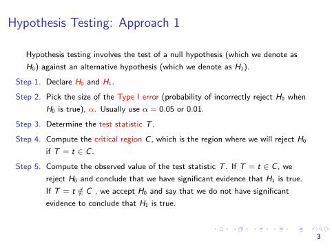
Hypothesis Testing: Approach 1
Hypothesis testing involves the test of a null hypothesis (which we denote as
H0) against an alternative hypothesis (which we denote as H1).
Step 1. Declare H0 and H1.
Step 2. Pick the size of the Type I error (probability of incorrectly reject H0 when
H0 is true), α. Usually use α = 0.05 or 0.01.
Step 3. Determine the test statistic T .
Step 4. Compute the critical region C , which is the region where we will reject H0
if T = t ∈ C .
Step 5. Compute the observed value of the test statistic T . If T = t ∈ C , we
reject H0 and conclude that we have significant evidence that H1 is true.
If T = t /∈ C , we accept H0 and say that we do not have significant
evidence to conclude that H1 is true.
3
Hypothesis Testing: Approach 1
More on Step 4:
Type I error =Prob(reject the null hypothesis | H0 is true)
=Prob(T ∈ C | H0 is true)
≤α.
4

Practice problem 1
Practice problem 1
Suppose we are interested in testing the (null) hypothesis that a newborn baby
is equally likely to be a boy or a girl. To test this hypothesis, we take a sample
of 10,000 newborn babies and observe 5,114 boys. Use (i) the proportion of
boys and (ii) the number of boys as test statistics and carry out two hypothesis
testings of the (null) hypothesis and the alternative that the probability of a
boy is not equal to the probability of a girl via the cut-off number approach
(α = 0.05).
5
Solution to practice problem 1
Solution
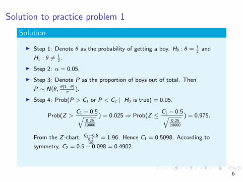
I Step 1: Denote θ as the probability of getting a boy. H0 : θ = 12
and
H1 : θ 6= 12.
I Step 2: α = 0.05.
I Step 3: Denote P as the proportion of boys out of total. Then
P ∼ N(θ, θ(1−θ)n
).
I Step 4: Prob(P > C1 or P < C2 | H0 is true) = 0.05.
Prob(Z >C1 − 0.5√
0.2510000
) = 0.025⇒ Prob(Z ≤ C1 − 0.5√0.2510000
) = 0.975.
From the Z -chart, C1−0.50.5100
= 1.96. Hence C1 = 0.5098. According to
symmetry, C2 = 0.5− 0.098 = 0.4902.
I Step 5: p = 0.5114 > C1 reject the null hypothesis.
6
Solution to practice problem 1
Solution
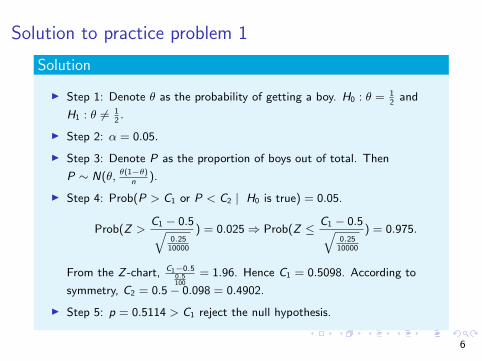
I Step 1: Denote θ as the probability of getting a boy. H0 : θ = 12
and
H1 : θ 6= 12.
I Step 2: α = 0.05.
I Step 3: Denote P as the proportion of boys out of total. Then
P ∼ N(θ, θ(1−θ)n
).
I Step 4: Prob(P > C1 or P < C2 | H0 is true) = 0.05.
Prob(Z >C1 − 0.5√
0.2510000
) = 0.025⇒ Prob(Z ≤ C1 − 0.5√0.2510000
) = 0.975.
From the Z -chart, C1−0.50.5100
= 1.96. Hence C1 = 0.5098. According to
symmetry, C2 = 0.5− 0.098 = 0.4902.
I Step 5: p = 0.5114 > C1 reject the null hypothesis.
6
Solution to practice problem 1
Solution
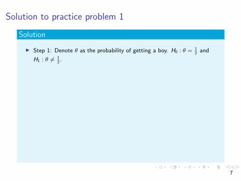
I Step 1: Denote θ as the probability of getting a boy. H0 : θ = 12
and
H1 : θ 6= 12.
I Step 2: α = 0.05.
I Step 3: Denote P as the proportion of boys out of total. Then
P ∼ N(θ, θ(1−θ)n
).
I Step 4: Prob(P > C1 or P < C2 | H0 is true) = 0.05.
Prob(Z >C1 − 0.5√
0.2510000
) = 0.025⇒ Prob(Z ≤ C1 − 0.5√0.2510000
) = 0.975.
From the Z -chart, C1−0.50.5100
= 1.96. Hence C1 = 0.5098. According to
symmetry, C2 = 0.5− 0.098 = 0.4902.
I Step 5: p = 0.5114 > C1 reject the null hypothesis.
6
Solution to practice problem 1
Solution
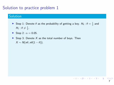
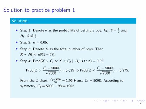
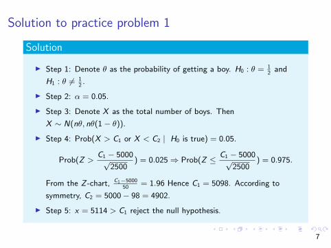
I Step 1: Denote θ as the probability of getting a boy. H0 : θ = 12
and
H1 : θ 6= 12.
I Step 2: α = 0.05.
I Step 3: Denote X as the total number of boys. Then
X ∼ N(nθ, nθ(1− θ)).
I Step 4: Prob(X > C1 or X < C2 | H0 is true) = 0.05.
Prob(Z >C1 − 5000√
2500) = 0.025⇒ Prob(Z ≤ C1 − 5000√
2500) = 0.975.
From the Z -chart, C1−500050
= 1.96 Hence C1 = 5098. According to
symmetry, C2 = 5000− 98 = 4902.
I Step 5: x = 5114 > C1 reject the null hypothesis.
7

Solution to practice problem 1
Solution
I Step 1: Denote θ as the probability of getting a boy. H0 : θ = 12
and
H1 : θ 6= 12.
I Step 2: α = 0.05.
I Step 3: Denote X as the total number of boys. Then
X ∼ N(nθ, nθ(1− θ)).
I Step 4: Prob(X > C1 or X < C2 | H0 is true) = 0.05.
Prob(Z >C1 − 5000√
2500) = 0.025⇒ Prob(Z ≤ C1 − 5000√
2500) = 0.975.
From the Z -chart, C1−500050
= 1.96 Hence C1 = 5098. According to
symmetry, C2 = 5000− 98 = 4902.
I Step 5: x = 5114 > C1 reject the null hypothesis.
7
Practice Problem 2
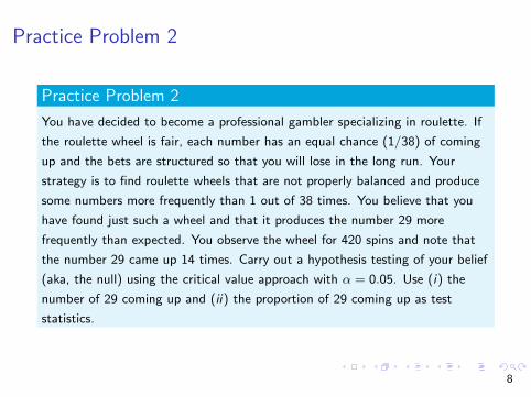
Practice Problem 2
You have decided to become a professional gambler specializing in roulette. If
the roulette wheel is fair, each number has an equal chance (1/38) of coming
up and the bets are structured so that you will lose in the long run. Your
strategy is to find roulette wheels that are not properly balanced and produce
some numbers more frequently than 1 out of 38 times. You believe that you
have found just such a wheel and that it produces the number 29 more
frequently than expected. You observe the wheel for 420 spins and note that
the number 29 came up 14 times. Carry out a hypothesis testing of your belief
(aka, the null) using the critical value approach with α = 0.05. Use (i) the
number of 29 coming up and (ii) the proportion of 29 coming up as test
statistics.
8
Solution to practice problem 2
Solution
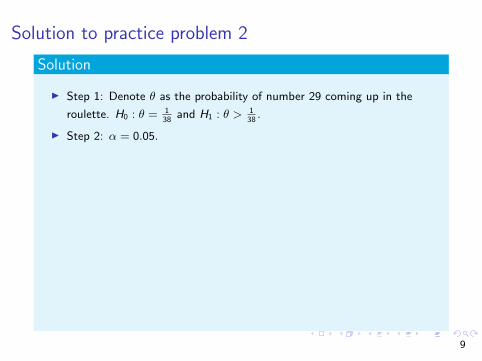
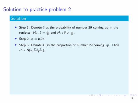
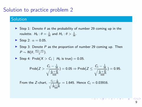
I Step 1: Denote θ as the probability of number 29 coming up in the
roulette. H0 : θ = 138
and H1 : θ > 138.
I Step 2: α = 0.05.
I Step 3: Denote P as the proportion of number 29 coming up. Then
P ∼ N(θ, θ(1−θ)n
).
I Step 4: Prob(X > C1 | H0 is true) = 0.05.
Prob(Z >C1 − 1
38√138× 37
38420
) = 0.05⇒ Prob(Z ≤C1 − 1
38√138× 37
38420
) = 0.95.
From the Z -chart,C1− 1
38√138
× 3738
420
= 1.645. Hence C1 = 0.03916.
I Step 5: p = 14420
= 0.03333 < C1 don’t reject the null hypothesis.
9
Solution to practice problem 2
Solution
I Step 1: Denote θ as the probability of number 29 coming up in the
roulette. H0 : θ = 138
and H1 : θ > 138.
I Step 2: α = 0.05.
I Step 3: Denote P as the proportion of number 29 coming up. Then
P ∼ N(θ, θ(1−θ)n
).
I Step 4: Prob(X > C1 | H0 is true) = 0.05.
Prob(Z >C1 − 1
38√138× 37
38420
) = 0.05⇒ Prob(Z ≤C1 − 1
38√138× 37
38420
) = 0.95.
From the Z -chart,C1− 1
38√138
× 3738
420
= 1.645. Hence C1 = 0.03916.
I Step 5: p = 14420
= 0.03333 < C1 don’t reject the null hypothesis.
9
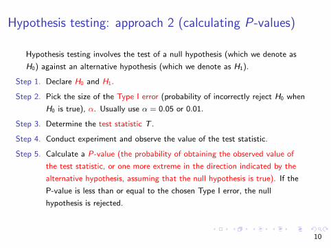
Hypothesis testing: approach 2 (calculating P-values)
Hypothesis testing involves the test of a null hypothesis (which we denote as
H0) against an alternative hypothesis (which we denote as H1).
Step 1. Declare H0 and H1.
Step 2. Pick the size of the Type I error (probability of incorrectly reject H0 when
H0 is true), α. Usually use α = 0.05 or 0.01.
Step 3. Determine the test statistic T .
Step 4. Conduct experiment and observe the value of the test statistic.
Step 5. Calculate a P-value (the probability of obtaining the observed value of
the test statistic, or one more extreme in the direction indicated by the
alternative hypothesis, assuming that the null hypothesis is true). If the
P-value is less than or equal to the chosen Type I error, the null
hypothesis is rejected.
10
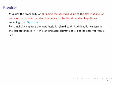
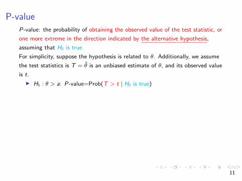
P-valueP-value: the probability of obtaining the observed value of the test statistic, or
one more extreme in the direction indicated by the alternative hypothesis,
assuming that H0 is true.
For simplicity, suppose the hypothesis is related to θ. Additionally, we assume
the test statistics is T = θ̂ is an unbiased estimate of θ, and its observed value
is t.
I H1 : θ > a: P-value=Prob(T > t | H0 is true)
I H1 : θ < a: P-value=Prob(T < t | H0 is true)
I H1 : θ 6= a:
P-value = Prob(|T − a| > |t − a| | H0 is true)
=Prob(T > a + |t − a| | H0 is true) + Prob(T < a− |t − a| | H0 is true)
=2 · Prob(T > a + |t − a| | H0 is true)
=
2 · Prob(T > t | H0 is true), t > a (upward)
2 · Prob(T < t | H0 is true), t < a (downward)
(If T = θ̂ is symmetric around θ, and usually it is. )
11
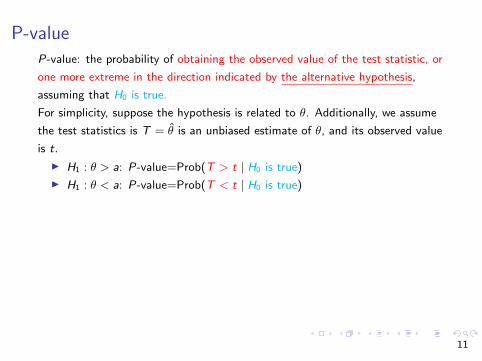
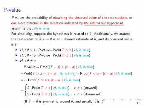
P-valueP-value: the probability of obtaining the observed value of the test statistic, or
one more extreme in the direction indicated by the alternative hypothesis,
assuming that H0 is true.
For simplicity, suppose the hypothesis is related to θ. Additionally, we assume
the test statistics is T = θ̂ is an unbiased estimate of θ, and its observed value
is t.
I H1 : θ > a: P-value=Prob(T > t | H0 is true)
I H1 : θ < a: P-value=Prob(T < t | H0 is true)
I H1 : θ 6= a:
P-value = Prob(|T − a| > |t − a| | H0 is true)
=Prob(T > a + |t − a| | H0 is true) + Prob(T < a− |t − a| | H0 is true)
=2 · Prob(T > a + |t − a| | H0 is true)
=
2 · Prob(T > t | H0 is true), t > a (upward)
2 · Prob(T < t | H0 is true), t < a (downward)
(If T = θ̂ is symmetric around θ, and usually it is. ) 11
Practice Problem 3
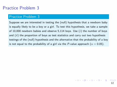
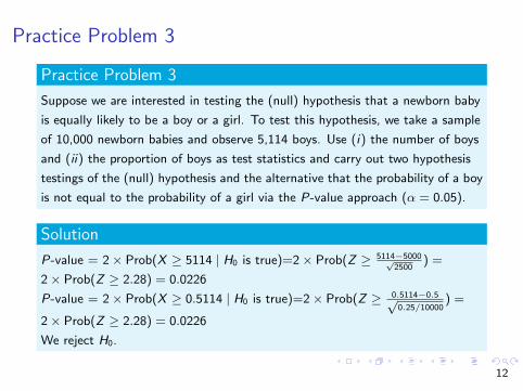
Practice Problem 3
Suppose we are interested in testing the (null) hypothesis that a newborn baby
is equally likely to be a boy or a girl. To test this hypothesis, we take a sample
of 10,000 newborn babies and observe 5,114 boys. Use (i) the number of boys
and (ii) the proportion of boys as test statistics and carry out two hypothesis
testings of the (null) hypothesis and the alternative that the probability of a boy
is not equal to the probability of a girl via the P-value approach (α = 0.05).
Solution
P-value = 2× Prob(X ≥ 5114 | H0 is true)=2× Prob(Z ≥ 5114−5000√2500
) =
2× Prob(Z ≥ 2.28) = 0.0226
P-value = 2× Prob(X ≥ 0.5114 | H0 is true)=2× Prob(Z ≥ 0.5114−0.5√0.25/10000
) =
2× Prob(Z ≥ 2.28) = 0.0226
We reject H0.
12
Practice Problem 3
Practice Problem 3
Suppose we are interested in testing the (null) hypothesis that a newborn baby
is equally likely to be a boy or a girl. To test this hypothesis, we take a sample
of 10,000 newborn babies and observe 5,114 boys. Use (i) the number of boys
and (ii) the proportion of boys as test statistics and carry out two hypothesis
testings of the (null) hypothesis and the alternative that the probability of a boy
is not equal to the probability of a girl via the P-value approach (α = 0.05).
Solution
P-value = 2× Prob(X ≥ 5114 | H0 is true)=2× Prob(Z ≥ 5114−5000√2500
) =
2× Prob(Z ≥ 2.28) = 0.0226
P-value = 2× Prob(X ≥ 0.5114 | H0 is true)=2× Prob(Z ≥ 0.5114−0.5√0.25/10000
) =
2× Prob(Z ≥ 2.28) = 0.0226
We reject H0.
12
Practice Problem 4
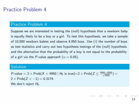
Practice Problem 4
Suppose we are interested in testing the (null) hypothesis that a newborn baby
is equally likely to be a boy or a girl. To test this hypothesis, we take a sample
of 10,000 newborn babies and observe 4,950 boys. Use (i) the number of boys
as test statistics and carry out two hypothesis testings of the (null) hypothesis
and the alternative that the probability of a boy is not equal to the probability
of a girl via the P-value approach (α = 0.05).
Solution
P-value = 2× Prob(X < 4950 | H0 is true)=2× Prob(Z ≤ 4950−5000√2500
) =
2× Prob(Z < −1) = 0.3174.
We don’t reject H0.
13
Deduction and Induction
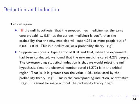
Critical region:
I “If the null hypothesis (that the proposed new medicine has the same
cure probability, 0.84, as the current medicine) is true”, then the
probability that the new medicine will cure 4,261 or more people out of
5,000 is 0.01. This is a deduction, or a probability theory “zig”.
I Suppose we chose a Type I error of 0.01 and that, when the experiment
had been conducted, we found that the new medicine cured 4,272 people.
The corresponding statistical induction is that we would reject the null
hypothesis, since the observed number cured (4,272) is in the critical
region. That is, it is greater than the value 4,261 calculated by the
probability theory “zig”. This is the corresponding induction, or statistical
“zag”. It cannot be made without the probability theory “zig”.
14

Deduction and Induction
P-value
I The statement “If the null hypothesis (that the proposed new medicine
has the same cure probability, 0.84, as the current medicine) is true”,
then the probability that the new medicine will cure 4,272 or more people
out of 5,000 is 0.0027 is a deduction, or a probability theory “zig”.
I When the experiment had been conducted, we found that the new
medicine cured 4,272 people. From the probability theory result just
calculated, the P-value is 0.0027. This is less than our chosen Type I
error of 0.01, so we reject the null hypothesis. This is the corresponding
induction, or statistical “zag”. It cannot be made without the probability
theory “zig” (which led to the P-value calculation of 0.0027).
15
Misc.
I We will learn Section 10 “ Tests on means” next week.
I Professor Ewens will take the recitation class next Friday.
16
Top Related