


γλώσσες
Σελίδες
Νομικός

Simple Linear Regression (OLS)
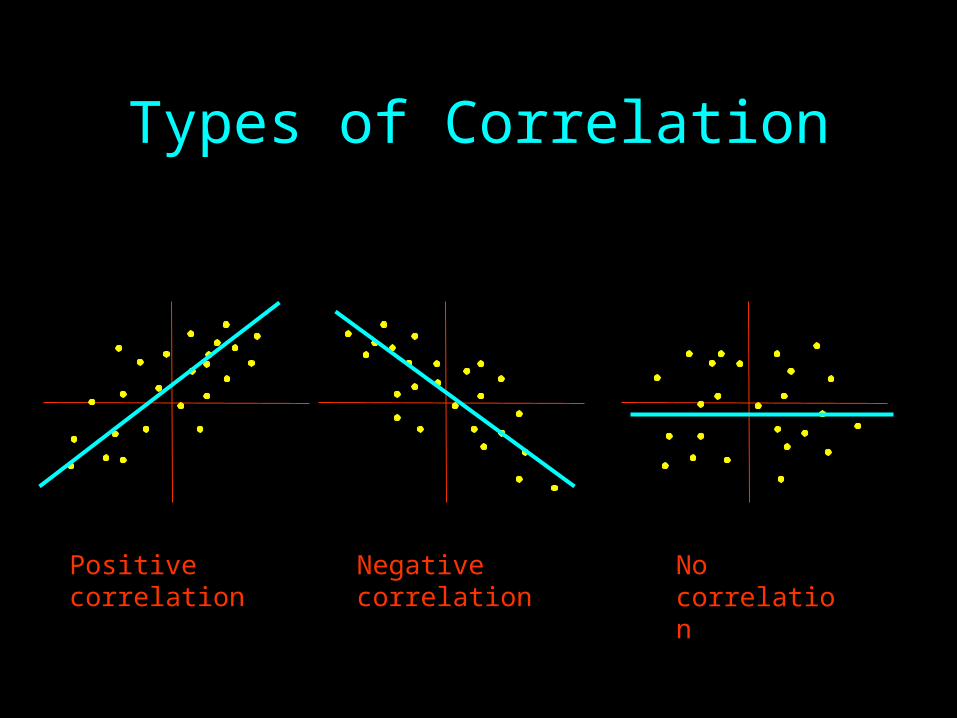
Types of Correlation
Positive correlation Negative correlation No correlation
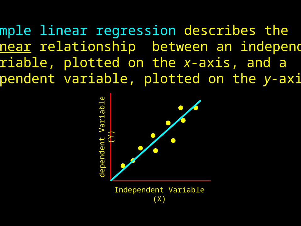
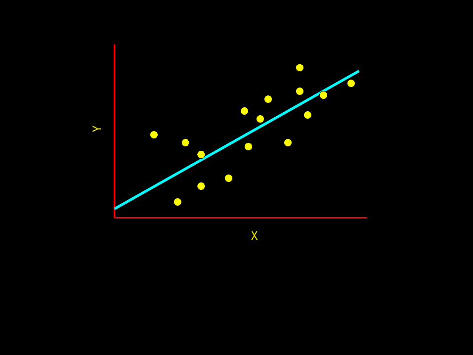
Simple linear regression describes the linear relationship between an independentvariable, plotted on the x-axis, and a dependent variable, plotted on the y-axis
Independent Variable (X)
depe
nden
t Var
iabl
e (Y
)
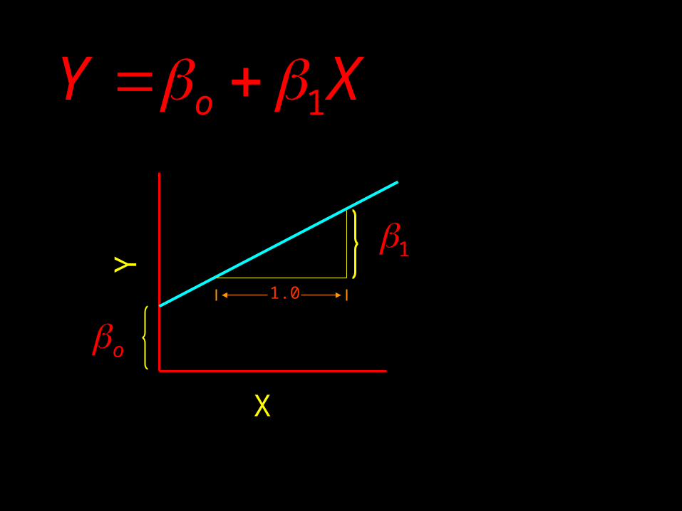
1oY X
X
Y
o1.0
1
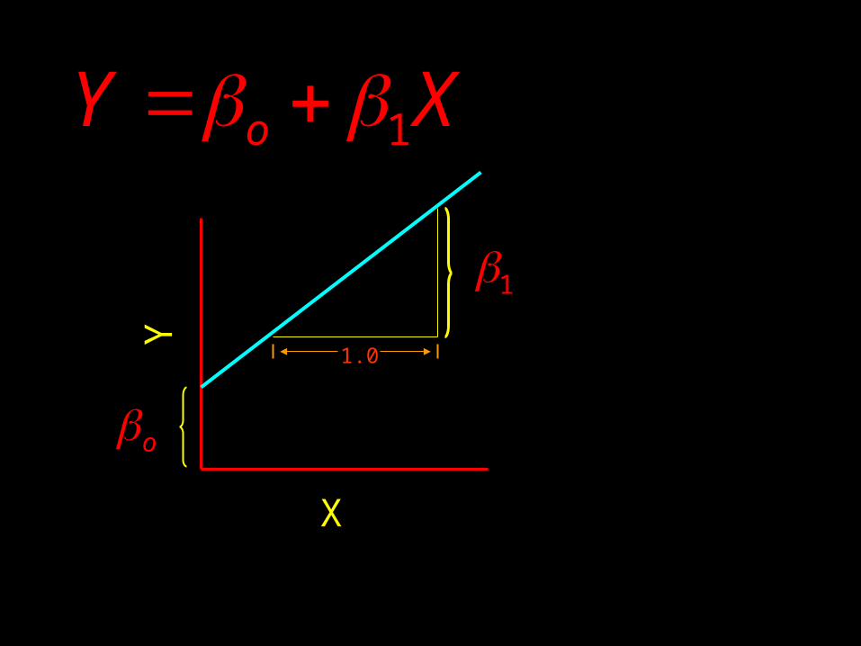
1oY X
X
Y
o
1.0
1
X
Y
X
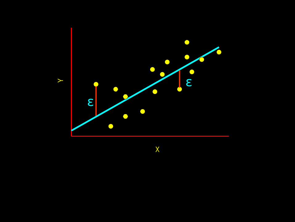
Y ε
ε
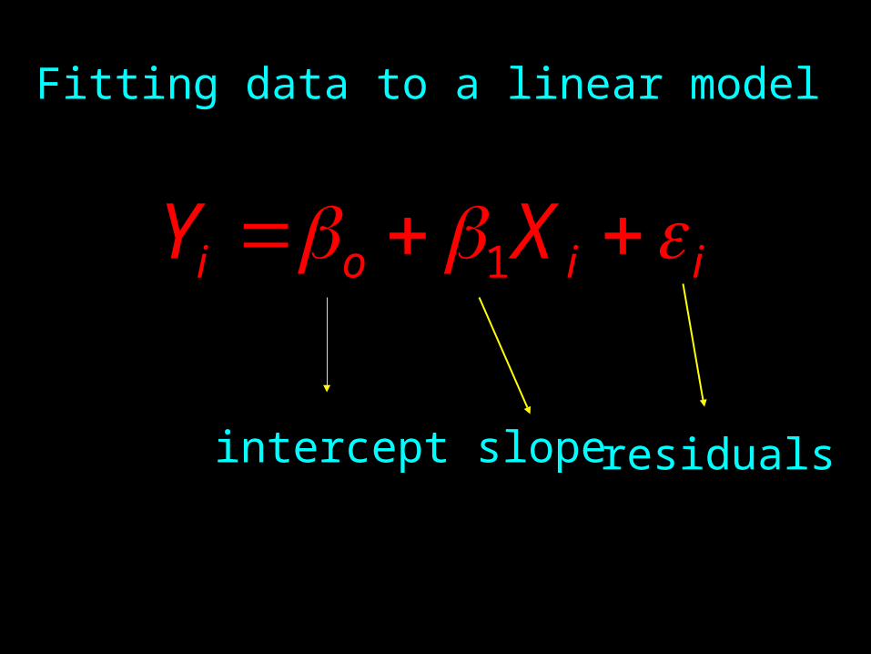
Fitting data to a linear model
1i o i iY X
intercept slope residuals
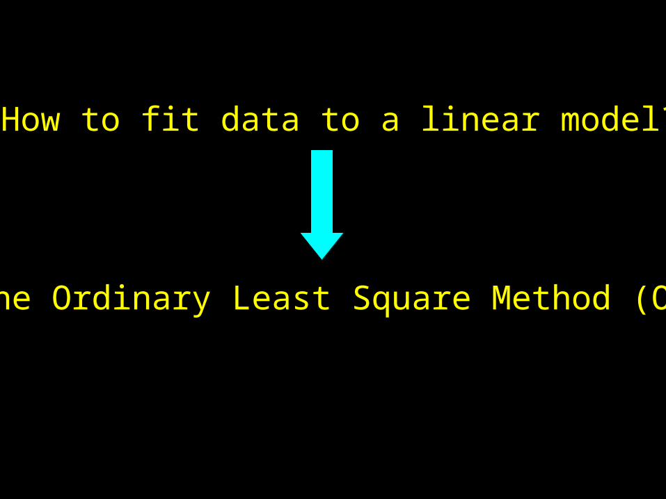
How to fit data to a linear model?
The Ordinary Least Square Method (OLS)
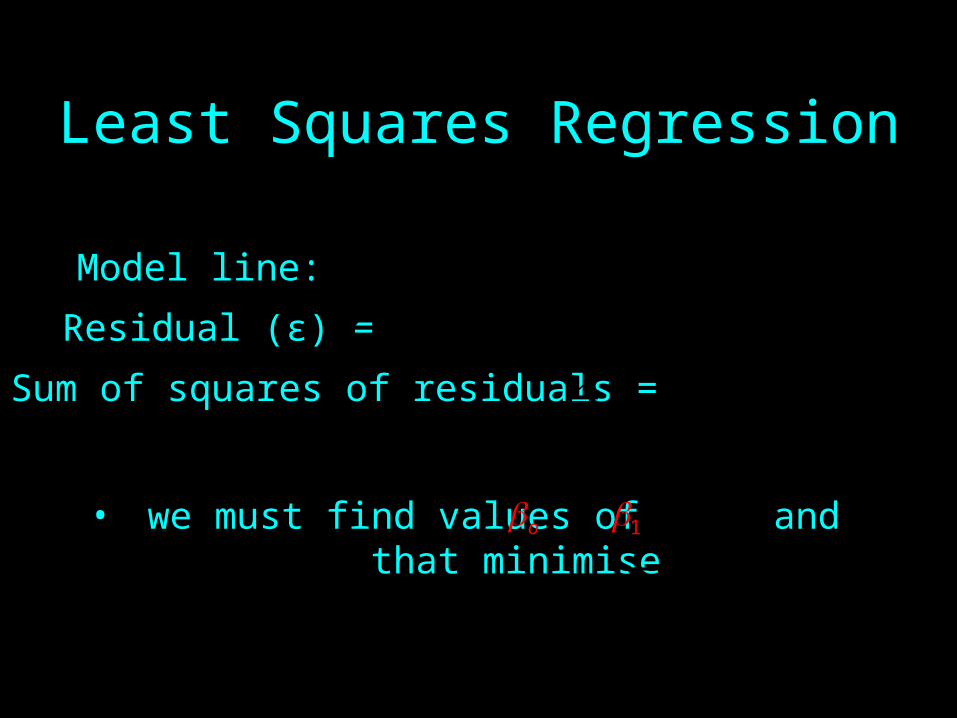
Least Squares Regression
Residual (ε) =
Sum of squares of residuals =
Model line:
• we must find values of and that minimise o 1
XY 10
YY
2)( YY
2)(min YY
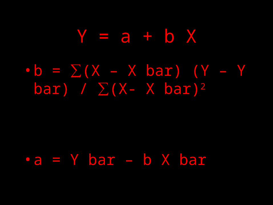
Y = a + b X
• b = ∑(X – X bar) (Y – Y bar) / ∑(X- X bar)2
• a = Y bar – b X bar
Regression Coefficients
21x
xy
xx
xy
S
Sb
XbYb 10

Required Statistics
nsobservatio ofnumber n
n
XX
n
YY
Descriptive Statistics
1
)( 1
2
n
YYYVar
n
i
1
)( 1
2
n
XXXVar
n
i
xxS
)(SSTS yy
xyS 1
),(Covar 1
n
YYXXYX
n
i
Regression Statistics
2)( YYSST
2)( YYSSR
2)( YYSSE
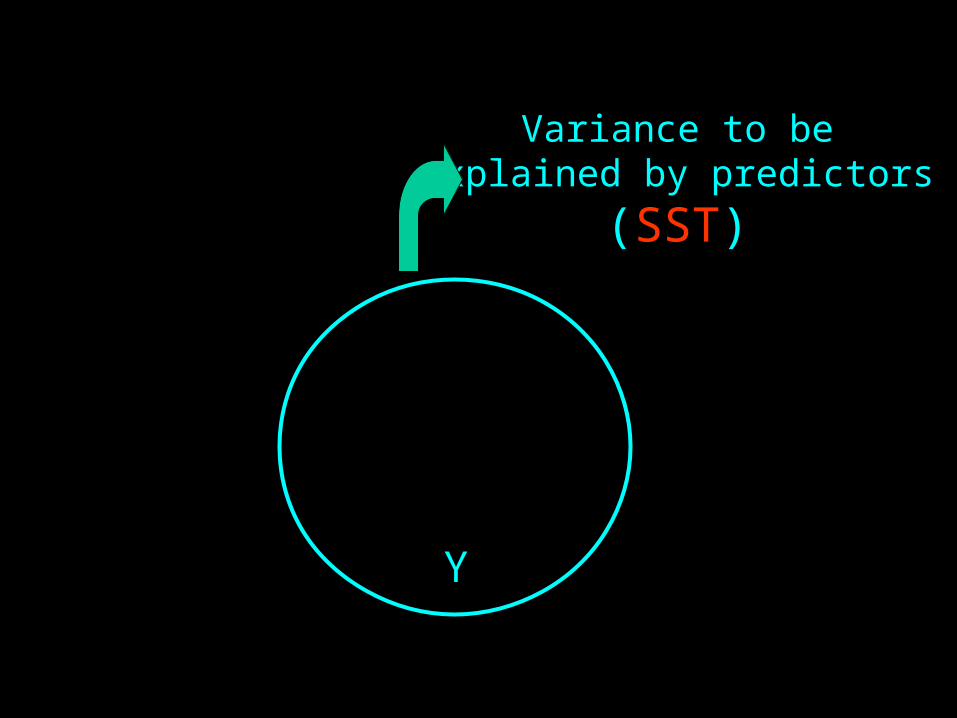
Y
Variance to beexplained by predictors
(SST)
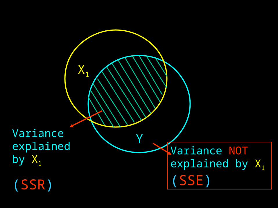
Y
X1
Variance NOT explained by X1
(SSE)
Variance explained by X1
(SSR)
SSESSRSST
Regression Statistics
Regression Statistics
SST
SSRR 2
Coefficient of Determinationto judge the adequacy of the regression model
Regression Statistics
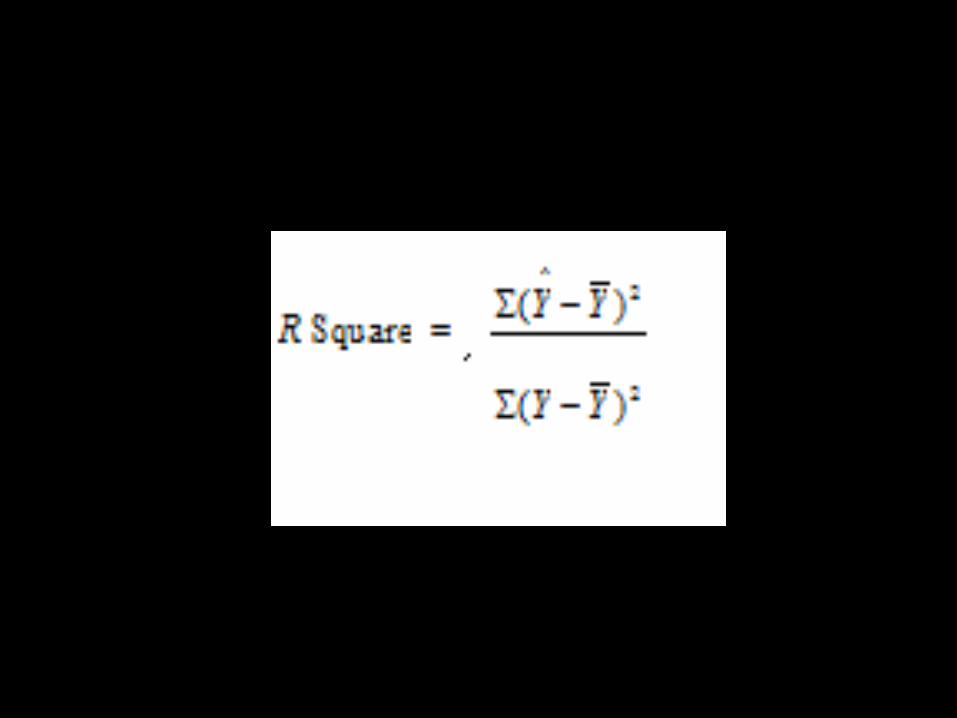
yx
xy
yyxx
xy
SS
SR
RR
2
Correlation
measures the strength of the linear association between two variables.
Standard Error for the regression model
MSES
n
SSES
SS
e
e
ee
2
2
22
2
Regression Statistics
2)( YYSSE
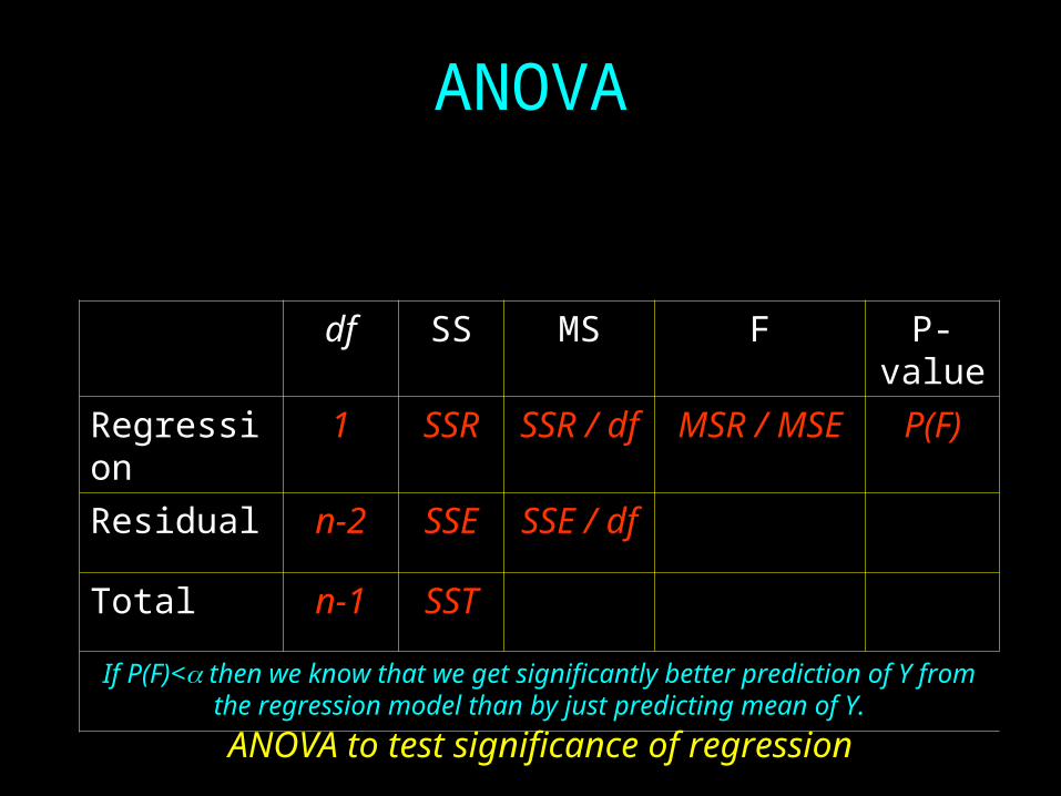
ANOVA
df SS MS F P-value
Regression 1 SSR SSR / df MSR / MSE P(F)
Residual n-2 SSE SSE / df
Total n-1 SST
If P(F)< then we know that we get significantly better prediction of Y from the regression model than by just predicting mean of Y.
ANOVA to test significance of regression
0:
0:
1
10
AH
H

Hypothesis Tests for Regression Coefficients
ib
iikn S
bt
)1(
0:
0:
1
0
i
i
H
H
Hypotheses Tests for Regression Coefficients
xx
eekn
SS
b
bS
bt
2
11
1
11)1( )(
0:
0:
1
10
AH
H

Hypothesis Tests on Regression Coefficients
xxe
ekn
SX
nS
b
bS
bt
22
00
0
00)1(
1)(
0:
0:
0
00
AH
H

Hypotheses Test the Correlation Coefficient
0:
0:0
AH
H
201
2
R
nRT
We would reject the null hypothesis if 2,2/0 ntt
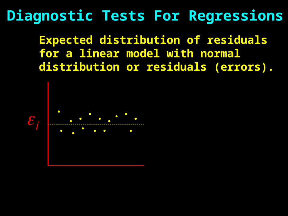
Diagnostic Tests For Regressions
i
Expected distribution of residuals for a linear model with normal distribution or residuals (errors).
iY
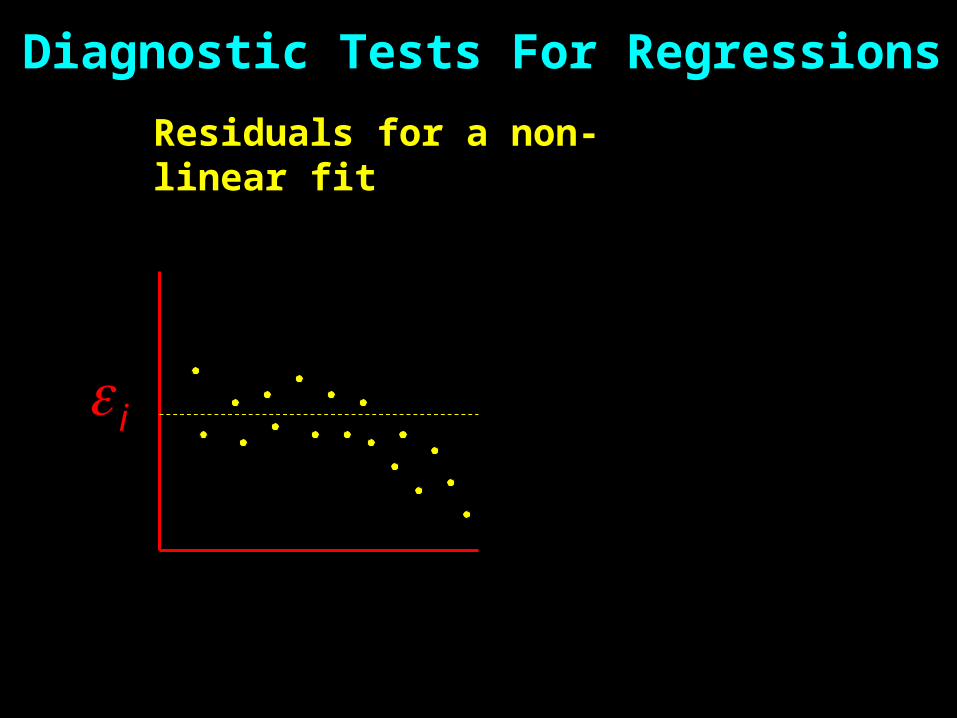
Diagnostic Tests For Regressions
i
Residuals for a non-linear fit
iY
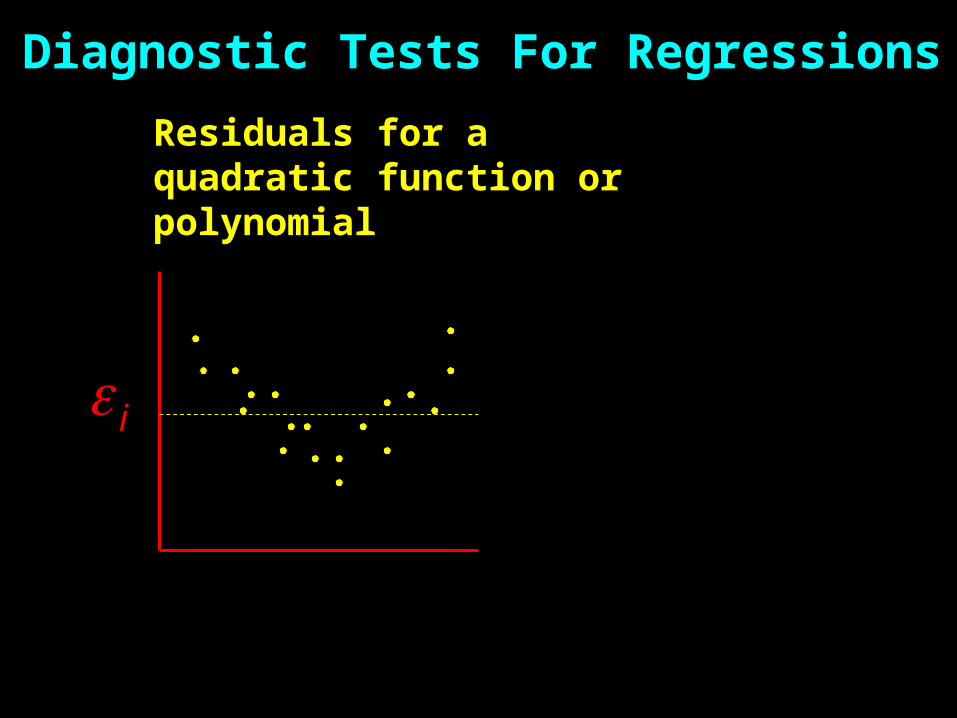
Diagnostic Tests For Regressions
i
Residuals for a quadratic function or polynomial
iY
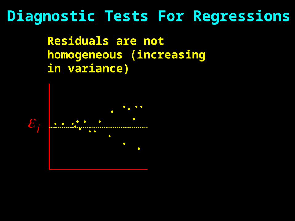
Diagnostic Tests For Regressions
i
Residuals are not homogeneous (increasing in variance)
iY
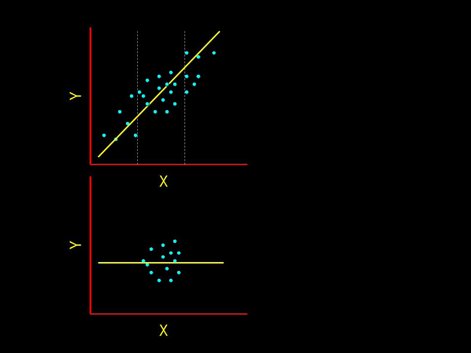
Regression – important points
1. Ensure that the range of valuessampled for the predictor variableis large enough to capture the fullrange to responses by the responsevariable.
X
Y
X
Y
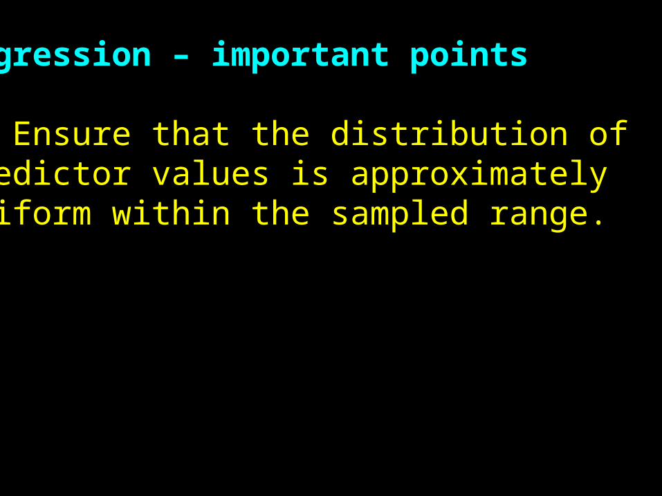
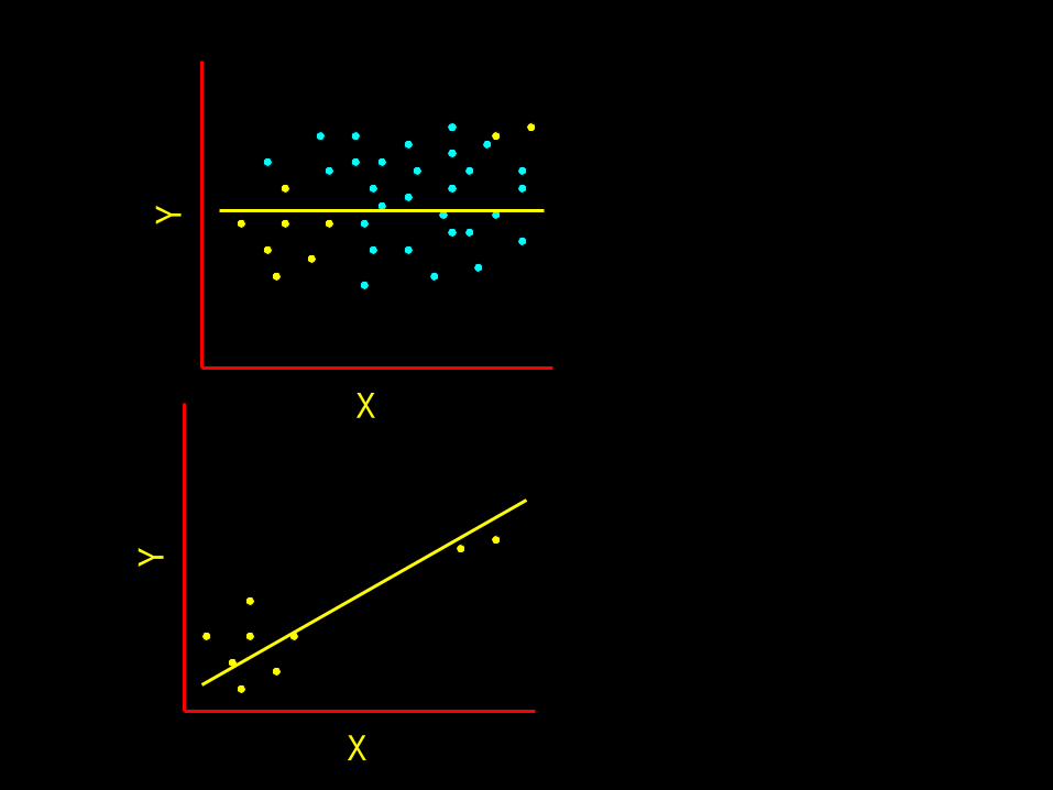
Regression – important points
2. Ensure that the distribution ofpredictor values is approximatelyuniform within the sampled range.
X
Y
X
Y
Assumptions of Regression
1. The linear model correctly describes the functional relationship between X and Y.
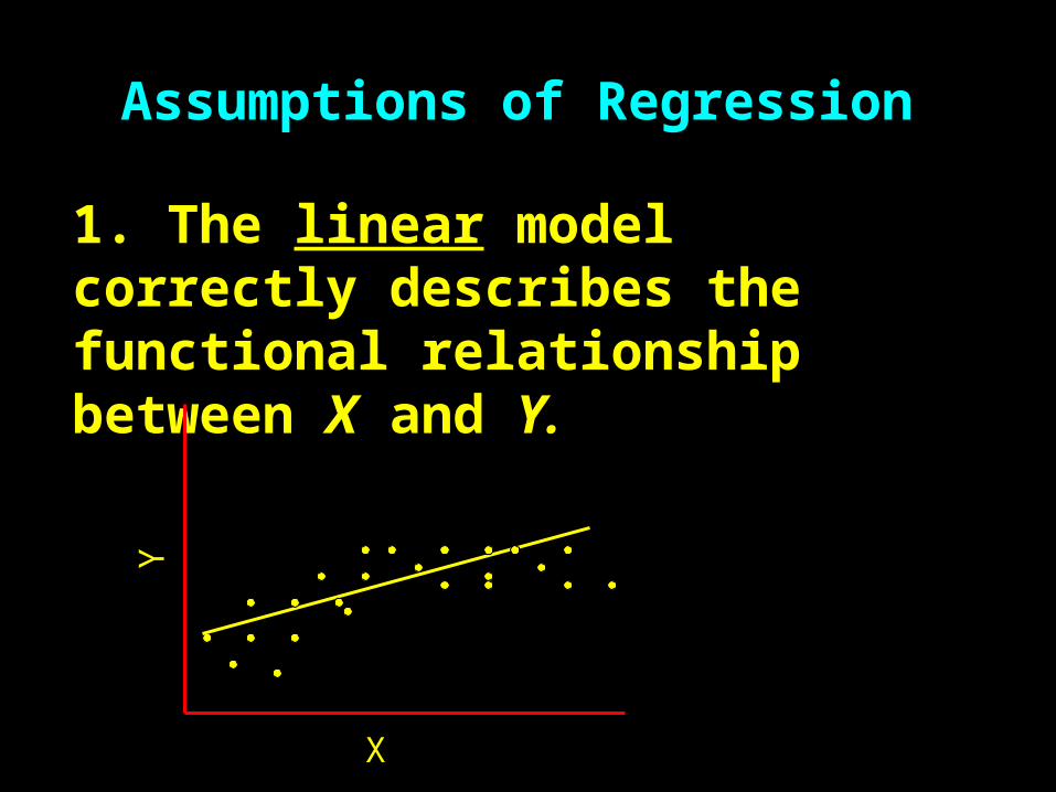
Assumptions of Regression
1. The linear model correctly describes the functional relationship between X and Y.
Y
X
Assumptions of Regression
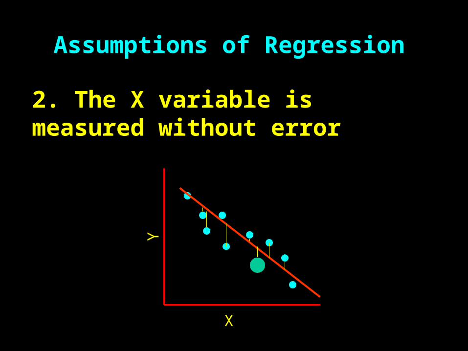
2. The X variable is measured without error
X
Y
Assumptions of Regression
3. For any given value of X, the sampled Y values are independent
4. Residuals (errors) are normally distributed.
5. Variances are constant along the regression line.
Multiple Linear Regression (MLR)
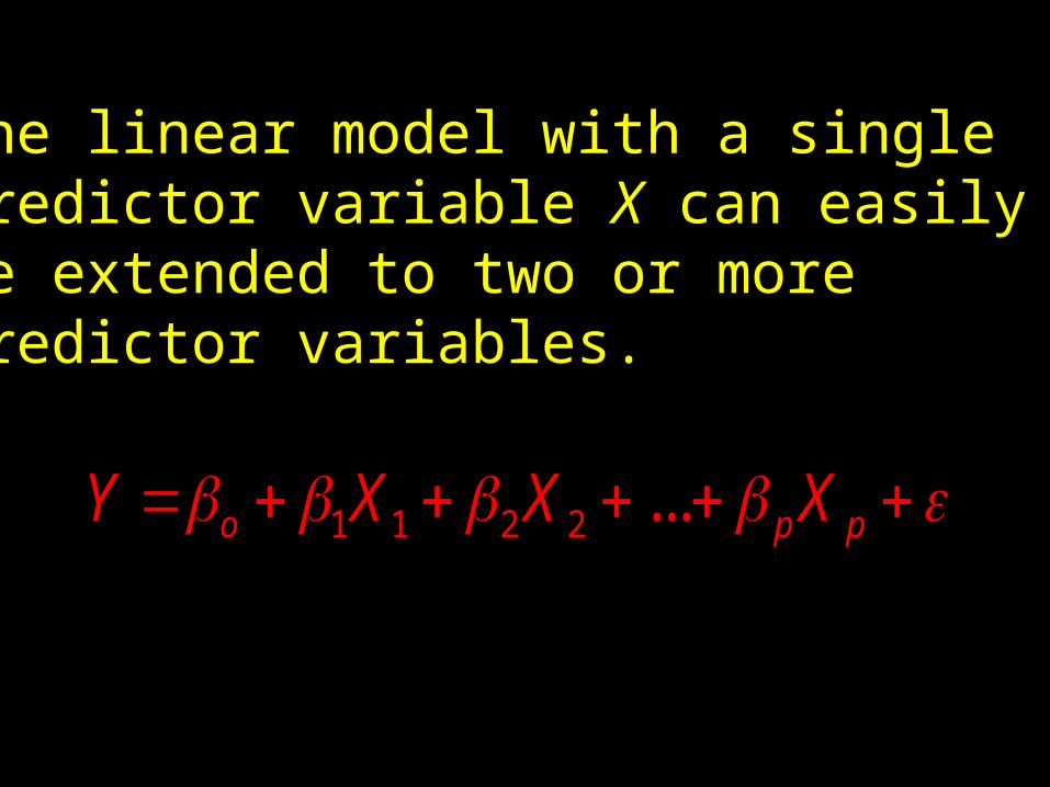
The linear model with a singlepredictor variable X can easily be extended to two or more predictor variables.
1 1 2 2 ...o p pY X X X
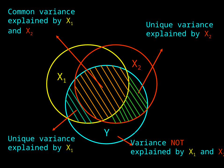
Y
X1
Variance NOT explained by X1 and X2
Unique variance explained by X1
Unique variance explained by X2
X2
Common variance explained by X1 and X2
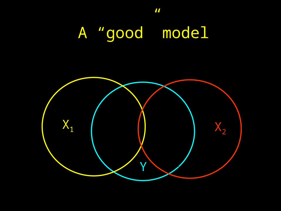
Y
X1 X2
A “good” model
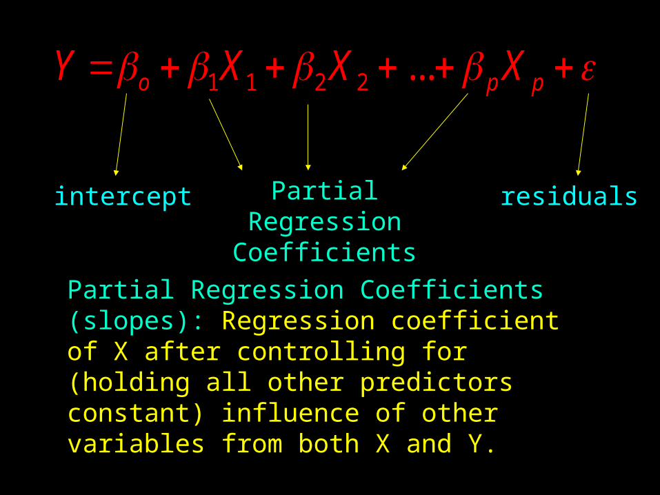
Partial Regression Coefficients (slopes): Regression coefficient of X after controlling for (holding all other predictors constant) influence of other variables from both X and Y.
1 1 2 2 ...o p pY X X X
Partial Regression Coefficients
intercept residuals
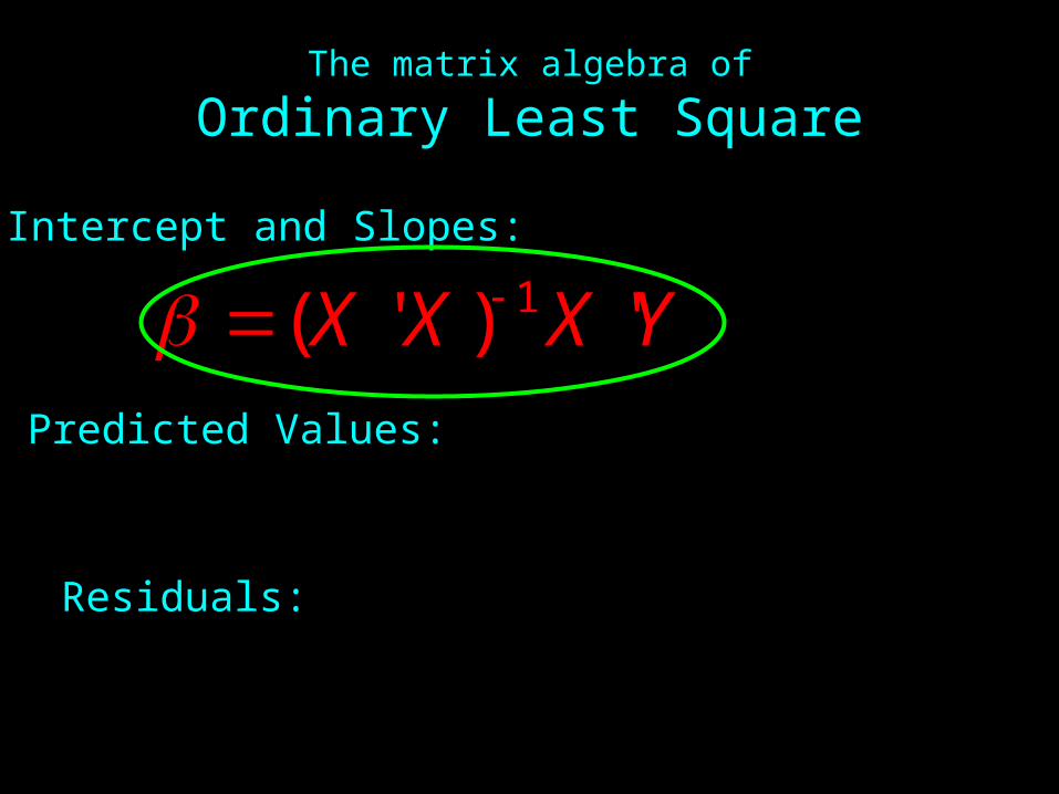
The matrix algebra of
Ordinary Least Square
1( ' ) 'X X X Y Predicted Values:
Residuals:
Intercept and Slopes:
XY
YY
Regression StatisticsHow good is our model?
2)( YYSST
2)( YYSSR
2)( YYSSE
Regression Statistics
SST
SSRR 2
Coefficient of Determinationto judge the adequacy of the regression model
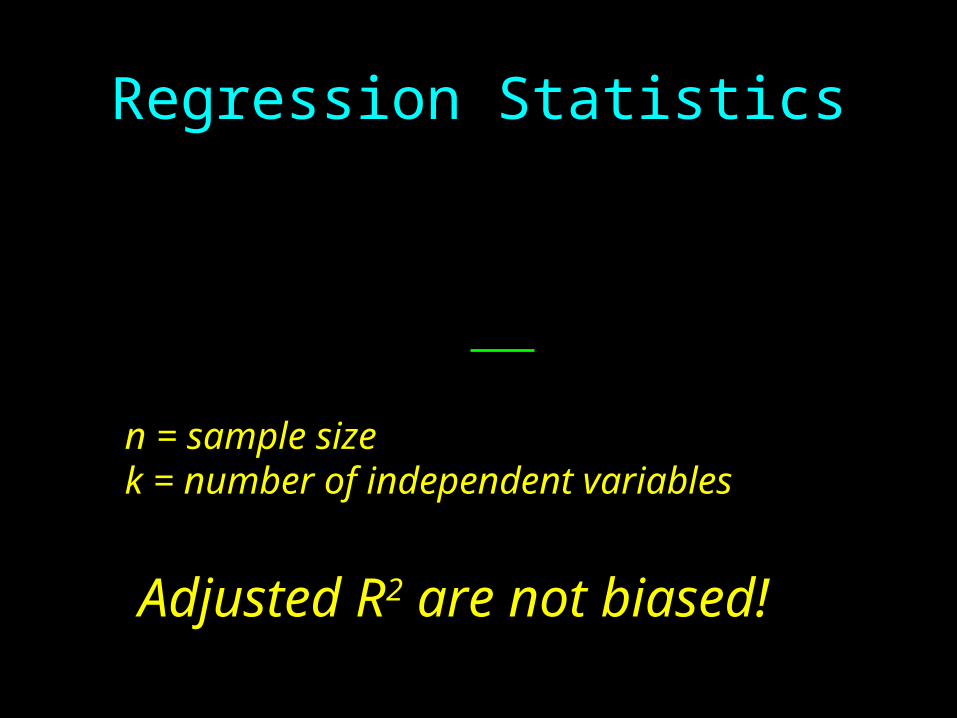
Adjusted R2 are not biased!
n = sample sizek = number of independent variables
)1(1
11 22 R
kn
nRadj
Regression Statistics
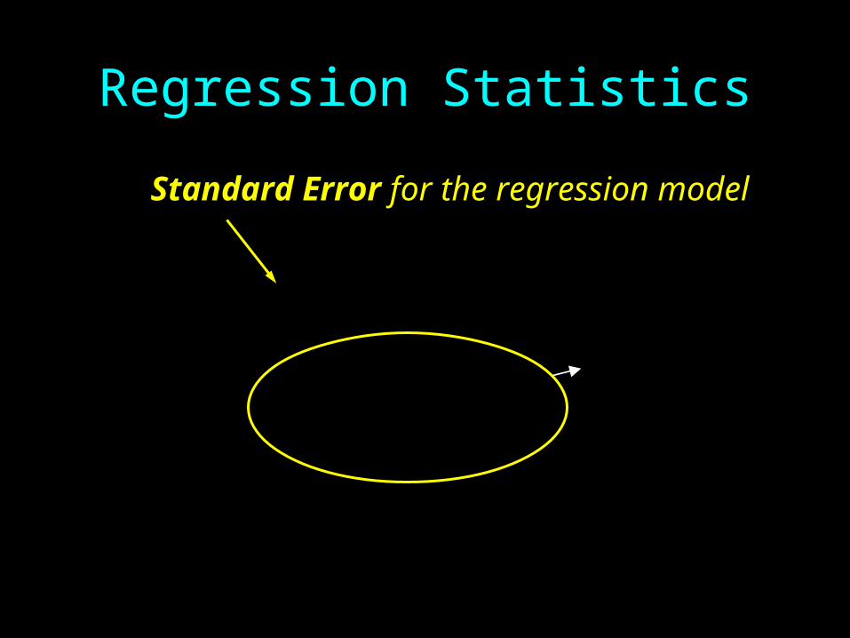
Standard Error for the regression model
MSES
kn
SSES
SS
e
e
ee
2
2
22
1
Regression Statistics
2)( YYSSE
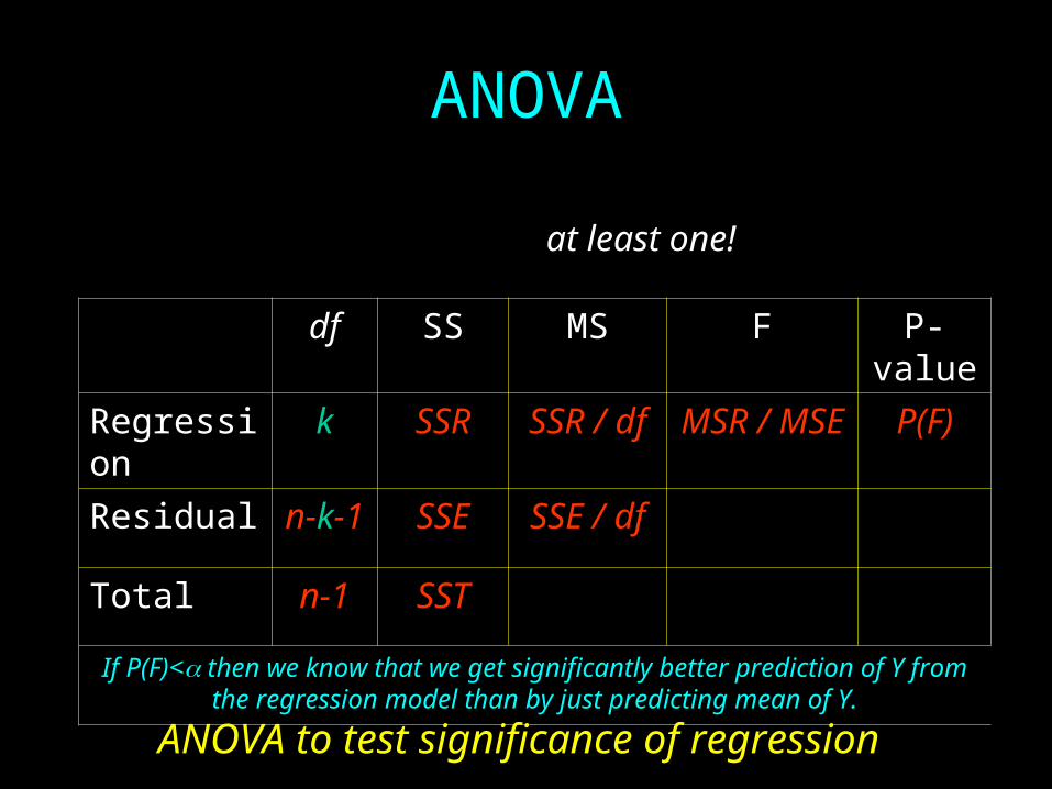
ANOVA
df SS MS F P-value
Regression k SSR SSR / df MSR / MSE P(F)
Residual n-k-1 SSE SSE / df
Total n-1 SST
If P(F)< then we know that we get significantly better prediction of Y from the regression model than by just predicting mean of Y.
ANOVA to test significance of regression
0:
0...: 210
iA
k
H
H
at least one!
Hypothesis Tests for Regression Coefficients
ib
iikn S
bt
)1(
0:
0:
1
0
i
i
H
H
Hypotheses Tests for Regression Coefficients
iie
ii
ie
ikn
CS
b
bS
bt
2
1)1( )(
0:
0:0
iA
i
H
H
xx
e
S
S 2
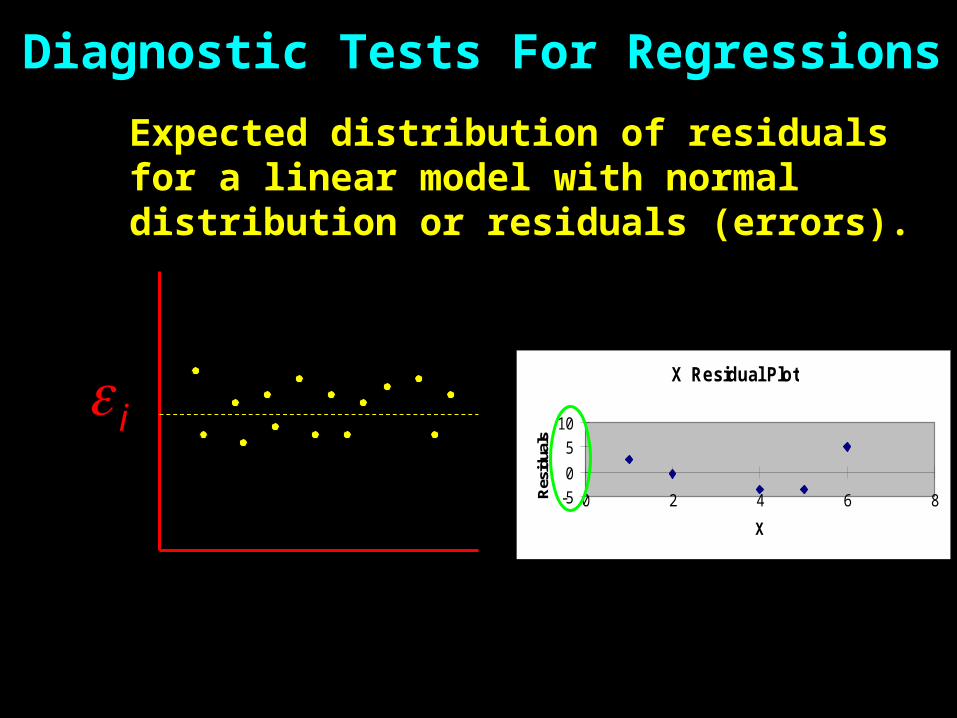
Diagnostic Tests For Regressions
i
Expected distribution of residuals for a linear model with normal distribution or residuals (errors).
iX
X Residual Plot
-5
0
5
10
0 2 4 6 8
XR
esid
uals
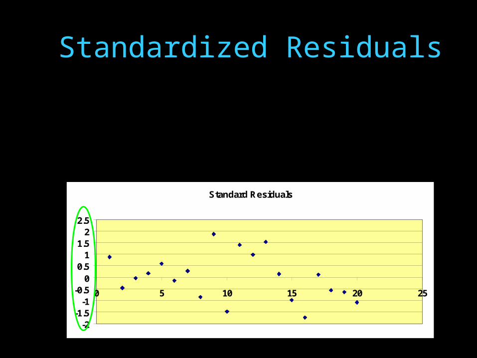
Standardized Residuals
2e
ii
S
ed
Standard Residuals
-2-1.5
-1-0.5
00.5
11.5
22.5
0 5 10 15 20 25
Avoiding predictors (Xs)
that do not contribute significantly
to model prediction
Model Selection

- Forward selectionThe ‘best’ predictor variables are entered, one by one.
- Backward eliminationThe ‘worst’ predictor variables are eliminated, one by one.
Model Selection
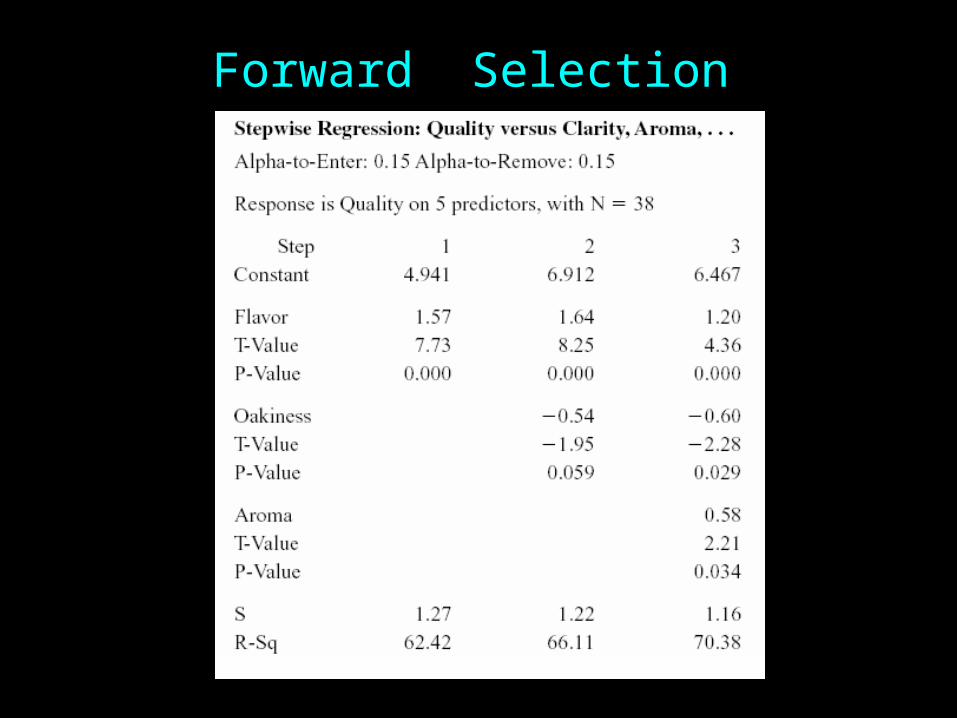
Forward Selection
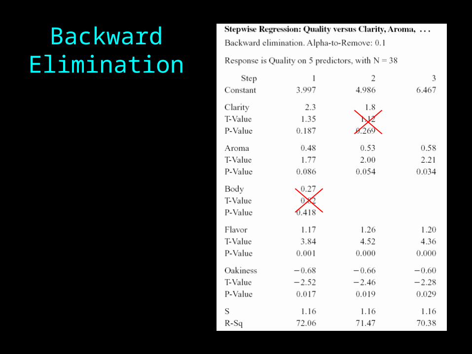
BackwardElimination

Model Selection: The General Case
1
),...,,,...,,(
),...,,,...,,(),...,,(
121
12121
kn
xxxxxSSEqk
xxxxxSSExxxSSE
Fkqq
kqqq
1,, knqkFF
zeronot in oneleast at :
0...:
1
210
H
H kqq
Reject H0 if :
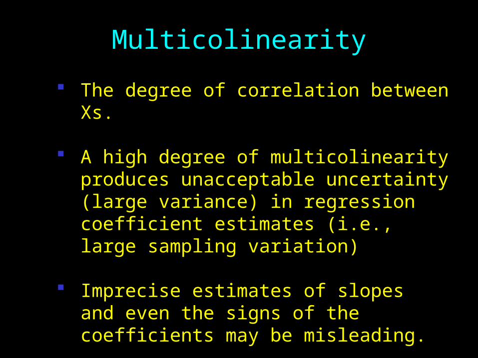
The degree of correlation between Xs.
A high degree of multicolinearity produces unacceptable uncertainty (large variance) in regression coefficient estimates (i.e., large sampling variation)
Imprecise estimates of slopes and even the signs of the coefficients may be misleading.
t-tests which fail to reveal significant factors.
Multicolinearity
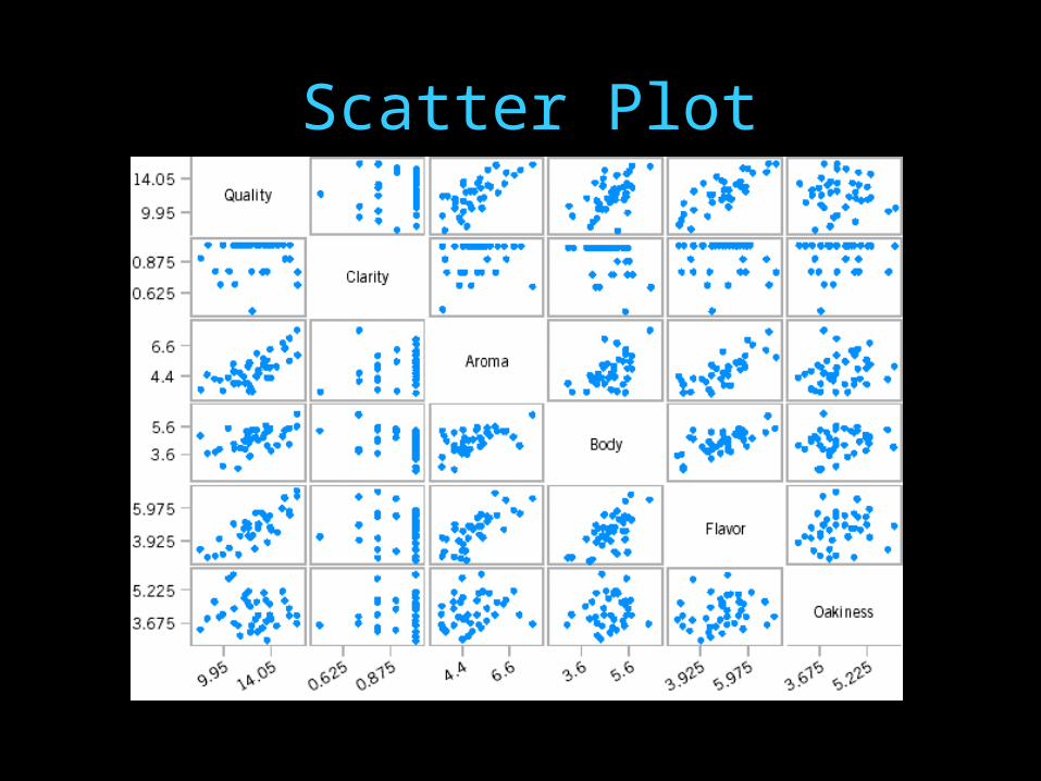
Scatter Plot
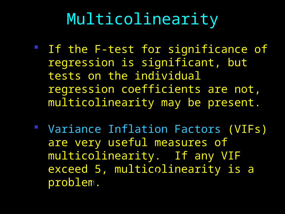
Multicolinearity
If the F-test for significance of regression is significant, but tests on the individual regression coefficients are not, multicolinearity may be present.
Variance Inflation Factors (VIFs) are very useful measures of multicolinearity. If any VIF exceed 5, multicolinearity is a problem.
iii
i CR
VIF
21
1)(

Thank You!
Top Related